Nonlinear response of runoff to atmospheric freezing level height variation based on hybrid prediction models

ABSTRACT

We use data on the freezing level height (FLH) and summer runoff in the Hotan River, China, from 1960 to 2013, to analyse the nonlinear relationships of atmospheric and hydrological factors at different time scales, by employing three nonlinear decomposition methods. Six hybrid prediction models are established by combining linear regression and back-propagation artificial neural network (BPANN) models. The decomposition results by three nonlinear methods are compared, indicating that the extreme-point symmetric mode decomposition (ESMD) method ensures the best prediction capacity. The runoff and FLH have periods of 3 and 6 years, respectively, at the inter-annual scale, which pass the significance test of 0.05 (P < 0.05) by using the Monte Carlo method, although there were slight differences in the periods at the inter-decadal scale. Among the six models, ESMD-BPANN exhibits the highest accuracy, with good reliability and resolution, according to several performance indicators. The ESMD-BPANN model is thus selected for the simulation and prediction of runoff.

KEYWORDS:

• nonlinear trend
• runoff prediction
• freezing level height
• ESMD-BPANN
• Hotan River Basin

Editor R. Woods; Associate editor A. Efstratiadis

1 Introduction

Hydroclimatic process modelling is one of the most important topics in hydrology and is an essential task in several water resources studies. Accurate modelling of hydroclimatic processes can provide important information for the environmental planning, land use and water resources management of a watershed. As a particular case, the arid region of northwest China (ARNC) is a sensitive area to climate change, since the ecosystem is extremely fragile and water resources originate mainly from mountain glacier-snow meltwater and precipitation (Shi et al. 2007, Wang et al. 2010). It is well understood that the relationship between climate change and runoff is extremely complex, owing to spatial and temporal variability of watershed characteristics (Chen et al. 2015), as well as the inherent nonlinear dynamics of the hydroclimatic system (Qin et al. 2018). Thus, modelling the hydroclimatic processes with nonlinear mechanism is a complex task.

A large number of studies have been undertaken to enhance our understanding of hydroclimatic processes. The modelling techniques can be broadly classified as theory-driven (i.e. conceptual and physically-based) and data-driven. The advantage of physically-based models is that it can reflect the physical mechanism of hydroclimatic processes. However, for a large river basin with sparse meteorological and hydrometric monitoring sites, as well as lacking of in situ data, it is difficult to estimate with acceptable accuracy the large number of input variables (e.g. precipitation, temperature, evapotranspiration, soil moisture, topography, land use, vegetation, etc.) for each grid cell (Xu et al. 2016, Wang et al. 2017). In this context, data-driven models, which can discover relationships from input-output data even when the user does not have a complete physical understanding of the underlying processes, may be preferable (Sudheer et al. 2010). While such models do not consider the physical mechanisms of the hydroclimatic processes, they are, in particular, very useful for river flow predictions, where the main concern is with making accurate predictions of runoff at specific river locations (Nayak et al. 2007).

In the last decades, there has been an increased interest in applying artificial neural network (ANN) (Modarres 2008, Kan et al. 2015, Tanty and Desmukh 2015, Daliakopoulos and Tsanis 2016, Kashani et al. 2016, Wang et al. 2017) and multiple linear regression (MLR) approaches (He et al. 2011, Garvelmann et al. 2015, Taguas et al. 2015, Ahani et al. 2017), which are the most common tools of data-driven models, to hydroclimatic processes simulation. The major reason for such an increasing interest in data-driven models is that they can be easily applied to a wide range of data types and can handle real-life uncertainty with low-cost solutions (Nayak et al. 2007).

While both these two computing techniques (ANN and MLR) have been proved to be effective when used on their own, there is still room to improve their prediction accuracy. The non-linear hydroclimatic series have obvious irregular fluctuations, which can be contaminated by various noise signals at different time scales (Wu et al. 2009). There is compelling evidence that the performance of prediction models can be improved by using signal decomposition methods to produce cleaner signals as model inputs (Tan et al. 2018). Based on this idea, several researchers have modelled runoff using nonlinear decomposition to establish hybrid prediction models (Huang et al. 2014, Nourani et al. 2014, Zhao and Chen 2015, Zhu et al. 2016, Ning et al. 2016, Zhao et al. 2017, Peng et al. 2017). For instance, Wang et al. (2014) established a hybrid model based on wavelet analysis (WA) combined with an auto-regressive model to predict daily runoff. The results indicated that this hybrid model provided more precise predictions than the single auto-regressive model. Based on WA, Xu et al. (2014) compared the simulation effect of MLR with a back-propagation artificial neural network (BPANN), and found that the latter method provided better simulations. Xu et al. (2016) proposed a hybrid model that integrates ensemble empirical mode decomposition (EEMD), BPANN, and a nonlinear regression equation to simulate annual runoff of the Kaidu River in ARNC, and concluded that this hybrid model was better than BPANN alone. Taken together, these studies illustrate that the development of a hybrid prediction model for runoff using nonlinear methods can characterize the nonlinear changes of hydroclimatic systems, although it is unclear whether WA or EEMD performs better in the simulation of the associated processes. Moreover, because of the rapid development of signal processing technology, Wang and Li (2013) proposed the use of extreme-point symmetric mode decomposition (ESMD), a method based on empirical mode decomposition (EMD), to process nonlinear time series. This new method has stronger self-adaptability and better characterizes local variations (Wang and Li 2014). However, ESMD has only rarely been used to study hydroclimatic systems. Qin et al. (2018) employed the ESMD method to analyse the spatial and temporal variation features of nonlinear precipitation trends in the arid region of northwest China from 1960 to 2015. The results indicate that the ESMD method can reflect integrated changes in the nonlinear trends of precipitation over different time scales.

In summary, the main aim of this study is to use different decomposition methods in order to investigate the nonlinear relationship of atmospheric and hydrological factors. We also evaluate the simulation accuracy of different hybrid models, especially the precision of novel hybrid models, which combine ESMD with different prediction models. A case study involving the simulation of Hotan River runoff is demonstrated to achieve these two goals. Given that most of this derives from glacier-snow meltwater from high mountains, many researchers have concluded that there is a close relationship between summer runoff and the freezing level height (FLH; altitude of the freezing layer) at different time scales (Wang et al. 2008a, Xu et al. 2011). To a certain extent, the rising or decreasing of FLH will influence the fluctuation of mountainous surface 0°C line, thus influencing the glacier-snow meltwater processes on high mountains (Zhang et al. 2010). In this paper, we propose combining ESMD with MLR and BPANN for ensemble prediction, and compare the simulation accuracy of three nonlinear decomposition methods – WA, EEMD and ESMD – in hybrid prediction models of summer runoff and FLH in the Hotan River. Then we select the hybrid model with the better precision to predict future runoff. The research results will provide an improved characterization of the nonlinear changes for this specific hydroclimatic system, and our methods may also help to improve the precision of runoff prediction.

2 Study area and research data

2.1 Study area

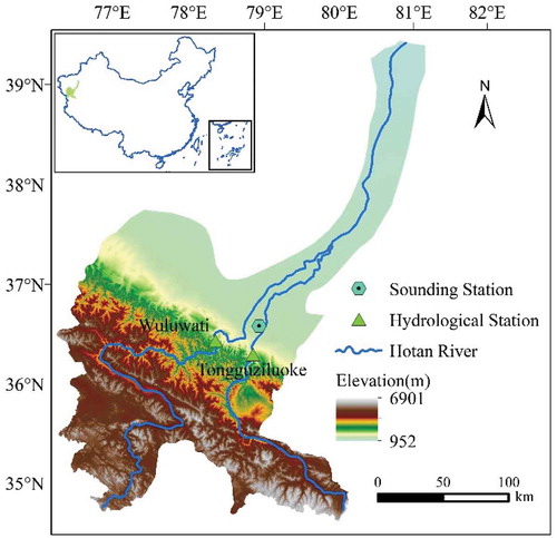
The Hotan River has a drainage area of 48 870 km² and is located south of the Tarim River Basin. It originates from the north slope of Kunlun Mountains and the Karakoram Mountains, and lies between the latitudes 34°52′ and 40°29′N and longitudes 77°25′ and 81°43′E (Fig. 1). The Hotan River has two tributaries: the east one is the Yurungkash River, which has a length of 513 km, an average annual runoff of 2195 hm³, and hosts the Tongguziluoke hydrological station in the mountain pass; the west tributary is the Karakash River, which has a length of 808 km, an average annual runoff of 2151 hm³, and hosts the Wuluwati hydrological station in the mountain pass. The summer runoff proportion of the two tributaries is as high as 80.7% and 72.9%, respectively (Wang et al. 2008a). The runoff of Hotan River mainly derives from glacier-snow meltwater, so temperature changes can have a great influence on runoff production. This region is in the hinterland of Eurasia, and has an extremely dry and warm temperate continental climate. The annual extreme maximum and minimum temperatures are 43.7 and – 28.9°C, respectively (Xu et al. 2011). The runoff recharge proportion from glacial meltwater in the Hotan River is up to about 57%, and the runoff recharge proportions from precipitation (including mixed rainfall and snow) and groundwater are approximately 23% and 20%, respectively (Yang 1991). The average annual potential evaporation is 817.8 mm (Hu et al. 2017).

Figure 1. Location of the Hotan River Basin in the arid region of northwest China, showing sounding stations, as well as Wuluwati and Tongguziluoke hydrological stations.

2.2 Data

The summer FLH can be calculated from monthly observations of sounding stations provided by the China Meteorological Administration in the ARNC, from June to August of the period 1960–2013. The mountainous area of the Hotan River has a high altitude (the average elevation is about 5000 m, Li et al. 2018), and the ground meteorological data are sparse. Moreover, the altitude of the ground meteorological station is relatively low (for example, the station in Hotan is located at 1374 m), and it is difficult to reflect the climatic characteristics of high-altitude mountainous areas, so a ground sounding station is employed instead. In the ARNC, the China Meteorological Administration has eight sounding stations (Chen et al. 2012). Although there is only one sounding station near the Hotan River, it can broadly reflect the climate characteristics of mountainous areas with different elevations to a certain extent, and is relatively less affected by human activities (Li et al. 2018). The average FLH is approximately 4869 m from 1960 to 2013, which is roughly equivalent to the average elevation of the mountain area in Hotan River. Therefore, the FLH is considered useful to reveal the relationship between climate change and runoff, and it can be used to simulate the runoff. Average annual flows of the Hotan River in summer consist of the total-measured runoff at two flow stations across the main tributaries, Wuluwati and Tongguziluoke. Summer runoff data were from the local hydrological bureau. These data are less affected by human activities, and more representative of the actual runoff of the river.

3 Methodology

To analyse summer runoff and FLH at different time scales, the runoff and FLH series were standardized by Z-score formula used for transforming normal variates to standard score form before the training procedure:

$Z=\frac{x-\mu }{\sigma }$

where x is the original data value, and μ and σ are the sample mean and standard deviation, respectively. The transformed variable has a zero mean and unit standard deviation, and retains the variability of the original data set.

For calibration and validation, the whole data series was divided into two periods: the calibration period (1960–2001), which was used for parameter estimation, and the validation period (2002–2013), which was to assess the predictive capacity of the model.

3.1 FLH calculation

The summer FLH is calculated using the following steps (Chen et al. 2012, Zhao et al. 2013):

1. Daily temperatures and FLH are available for three standard pressure levels of 500, 700, and 850 hPa at 00:00 and 12:00 h. It can be seen that the summer freezing layer is basically between two standard pressure levels of 850 and 500 hPa. The lower (850 hPa) and upper (500 hPa) standard pressure levels at 00:00 and 12:00 h are determined based on the locations of the river basin.

2. A linear interpolation method (Zhang and Guo 2011, Bradley et al. 2012) was used to compute the FLH at the two times (assuming the temperature between the two standard pressure levels of 500 and 850 hPa changes linearly in the vertical direction). Afterwards, the mean FLH values of two times were computed to obtain a daily FLH.

3. Daily FLH values between June and August were averaged to obtain the summer FLH. A linear interpolation method was used to compute the FLH, using the following equation:

$H_l=\frac{H_m-H_n}{T_m-T_n}\left(T_l-T_n\right)+H_n$

where T is the temperature (°C), H is the height (m), subscript l is the index of the freezing layer, and m and n are the indices of upper and lower standard pressure levels of freezing layer, respectively.

3.2 Construction of hybrid models

3.2.1 Decomposition methods

To investigate the nonlinear relationship of atmospheric and hydrological factors, the ESMD method was employed. This method originates from the EMD, provides better local characterizations, and it also has self-adaptability. It uses EMD to transform the external envelope symmetric interpolation method into the internal extreme-point symmetric interpolation method. The last mode is optimized using a least-squares method to generate an adaptive global mean curve. This is a direct interpolation method that considers the inherent deficiencies of integral transforms, in contrast to the more traditional method of spectrum analysis. ESMD directly determines the instantaneous frequencies and amplitudes. The advantages, disadvantages, and principles of the ESMD are described by Wang and Li (2013). The statistical significance of different components was tested based on the Monte Carlo method proposed by Wu and Huang (2004).

Qin et al. (2018) indicated that both the ESMD and EEMD can provide reliable decomposition results. In addition, WA has been widely applied to decompose the nonlinear time series (Nourani et al. 2014, Peng et al. 2017, Sang et al. 2018). Therefore, in order to compare the decomposition effects of EEMD and WA with those of ESMD, three different nonlinear decomposition methods are used to decompose atmospheric and hydrological time series.

Huang et al. (2009; see also Wu et al. 2007, Huang and Wu 2008) proposed the EEMD method to overcome the scale-mixing problem of the EMD method, which defines the true intrinsic mode function (IMF) components as the mean of an ensemble of trials, each consisting of the signal plus a white noise of finite amplitude. In this method, Gaussian white noise was first added to the data to make the signal continuous and reduce mode mixing at different time scales. The algorithm for EEMD can be found in Wu and Huang (2009). In principal, any signal P(t) can be decomposed into multiple IMFs and one residual (RES), as follows:

$P(t)=\sum _j{m}_j(t)+r(t)$

where m_j(t) (j = 1, 2, …) represents the signal’s components, sorted from higher frequency to lower frequency, and r(t) is the residual term, which represents the average trend of the signal. Each frequency varies with the signal P(t) and contains distinct components.

Wavelet analysis utilizes a wavelet function, known as mother wavelet, thus the continuous wavelet transformation of a discrete signal x(t) can be derived as (Kisi 2010):

$V_x(a,b)={\left|a\right|}^{-1/2}{\int }_{-\mathrm{\infty }}^{+\mathrm{\infty }}x(t){\mathrm{\Phi }}^{\ast }\left(\frac{t-b}{a}\right)\mathrm{d}t$

where ${\mathrm{\Phi }}^{\ast }$ indicates a complex conjugate function; V_x(a, b) is the matrix of wavelet coefficient; a and b represent the scale parameter and the translation parameter, respectively. The nonlinear time series x(t) can be decomposed at multiple scales based on the discrete wavelet transform (DWT). The DWT for signal x(t) can be represented as (Mallat 1989):

$x(t)=\sum _n{\mu }_{m_0,n}{\phi }_{m_0,n}(t)+\sum _{m=1}^{m_0}\sum _n{\omega }_{m,n}{\psi }_{m,n}(t)$

where ${\phi }_{m_0,n}(t)$ and ${\psi }_{m,n}(t)$ are the flexing and parallel shift of the scale of basic function, $\phi (t)$, and the mother wavelet function,$\mathrm{\Psi }(t)$, and ${\mu }_{m_0,n}(m<m_0)$ and ${\omega }_{m,n}$ are scaling and wavelet coefficients, respectively. More details concerning wavelet theory are available in Torrence and Compo (1998). The symmetrical wavelet (Symlet) is proposed as a basis function using the DWT to analyse time-series signals (Swee and Elangovan 1999). There are seven different Symlet functions from Symlet 2 to Symlet 8 (Yadav et al. 2015). The Symlet 8 provided robust results, and was used for approximating the patterns of summer runoff and FLH.

3.2.2 Prediction models

The BPANN has been applied in numerous real-world applications, including time series predictions (Abrahart et al. 2012). A three-layered BPANN includes several processing elements (nodes): an input layer, a hidden layer, and an output layer (Hsu et al. 1995). The form of the net input to unit (i) in the hidden and output layers is as follows (Maier and Dandy 1998):

$x_i=\sum _{j=1}^k{w}_{ji}{y}_j+{\theta }_i$

$I_j=f(x_i)$

where y_j is the input from each node in the previous layer, w_ji = (w_1i, w_2i, …, w_ki) is the connection weight, and k is the number of nodes. The connection weights are equal to the coefficients of the statistical models. The signals of the weighted input are summed and θ_i is the bias of unit i. Finally, x_i is weighted sum, which is then passed through a transfer function, f, to generate I_j (i.e. the output of the node).

At the tth time step, the error function of the network is adopted to calculate the sum of squared errors between output and target values, which is used to minimize the overall prediction error. The learning algorithm is as follows:

$F(t)=\frac{1}{2}\sum _{\hspace{0.17em}}^{\hspace{0.17em}}{\left[I_j(t)-d_j(t)\right]}^2$

where d_j(t) is the output value and I_j(t) is the target value, corresponding to jth neuron at tth moment, respectively. Figure 2 summarizes the back-propagation training process (Moghadassi et al. 2009). Any network can be trained if the transfer functions have derivative functions, net inputs, and weights (Kermani et al. 2005). The Levenberg-Marquardt optimization method was used, by employing standard functions offered in the MATLAB computing environment.

Figure 2. Schematic of the back-propagation training process.

In recent years, MLR models (He et al. 2011, Garvelmann et al. 2015, Taguas et al. 2015, Ahani et al. 2017) have also been employed to the prediction of runoff. In this study, MLR models were also developed to compare the performance of BPANN models.

3.2.3 Hybrid prediction models

For the comparison of the impacts of different nonlinear decomposition methods (ESMD, EEMD and WA) to the predictive capacity of the model, MLR and BPANN were used to obtain hybrid prediction models based on nonlinear decomposition.

Linear regression equations for the summer FLH (regarded as prediction factors) and runoff were established. The modelling period was 1960–2001, and the FLH time series 2002–2013 was substituted into the regression equation to assess its predictive capacity. The original sequence was established using stationary processing by different nonlinear decomposition methods (WA, EEMD and ESMD). The multivariate linear regression equations for the summer runoff and each component (decomposed by the FLH, 1960–2001) were established, and then each component (decomposed by the FLH, 2002–2013) was substituted into the regression equation for simulation of runoff. The simulated effect of the regression equation was tested, based on hybrid models of MLR and the three nonlinear decomposition methods.

A BPANN was used to simulate the runoff at each time scale, based on the decomposition results from WA, EEMD, and ESMD, taking ESMD as an example (Fig. 3). In this model, the open-loop neural network was simulated on the FLH data and runoff data from 1960–2013. The FLH at different time scales was the input layer, and the runoff at corresponding scales was the output one. The connection weights were adjusted using the training procedure, until the error was at a global minimum. Finally, the simulation results of runoff at different time scales were added to examine the fitting of the simulated values to the observed ones. The hybrid model with greatest predictive capacity was used to predict future runoff in the Hotan River. Initially, the FLH data for the period 2014–2030 were predicted by recursive strategy (Weigend and Gershenfeld 1994). Next, taking the FLH data from 2014–2030 as input, we switched to close-loop to perform a multi-year ahead prediction, and the output results were the predicted runoff data for the period 2014–2030.

Figure 3. Flowchart of the runoff prediction model based on the ESMD-BPANN algorithm.

3.3 Simulated effect test

To verify the validity of the simulated results, we calculated the correlation coefficients and employed the Student’s t-test to determine their statistical significance. The Akaike information criterion (AIC), which aims providing a balance among predictive capacity and parsimony (Anderson et al. 2000), was used to compare the goodness of fit between the hybrid models and the BPANN and MLR alone. The AIC is expressed as follows:

$\mathrm{R}\mathrm{S}\mathrm{S}=\sum _{i=1}^n{\left(P_i-Q_i\right)}^2$

$\mathrm{A}\mathrm{I}\mathrm{C}=2m+nln\left(\mathrm{R}\mathrm{S}\mathrm{S}/n\right)$

where n is the sample size; m is the number of parameters; P_i and Q_i are the actual data and simulated value of runoff, respectively. The root mean squared error (RMSE) and Nash-Sutcliffe efficiency (NSE) values were also calculated for each model, to evaluate its predictive capacity.

In addition to these deterministic metrics, posterior diagnostic tests were used to assess the reliability and resolution of the model prediction distributions. Prediction reliability describes how statistically consistent the time-varying prediction distribution is with the observed data, while resolution relates to how informative the predictions are and describes the average predictive capacity of the prediction distribution (Mason and Stephenson 2008, Humphrey et al. 2016). In particular, to compare prediction reliability of the different models, the Cronbach’s reliability index (Renard et al. 2010) was used through analysis of quantile-quantile (QQ) plots. The examples of predictive QQ plots displaying under-/over-confidence and under-/over-prediction is available in Laio and Tamea (2007). This index is correlated to the area between the 1:1 line and the p value curve and is given by:

$\alpha =1-2\frac{{\sum }_{t=1}^{N_t}\left|p_{Q_t}-p_{Q_t}^{\mathrm{t}\mathrm{h}}\right|}{N_t}$

where $p_{Q_t}$ is the observed p values of Q_t and $p_{Q_t}^{\mathrm{t}\mathrm{h}}$ is the theoretical p values of Q_t. The value of α varies between 0 and 1, where α = 1 represents perfect reliability, while α = 0 denotes fully unreliable forecast distributions.

Additionally, the relative resolution metric proposed by Renard et al. (2010) was used to quantify forecast resolution, which is computed as follows:

${\pi }^{(\mathrm{r}\mathrm{e}\mathrm{l})}=\frac{1}{N}\sum _{t=1}^N\frac{Q_{\mathrm{m}\mathrm{e}\mathrm{d},\mathrm{t}}}{Q_{\mathrm{s}\mathrm{d},\mathrm{t}}}$

where Q_med,t and Q_sd,t are the median and standard deviation of the simulated runoff distribution at time t, respectively. It is of great importance to consider both the reliability and resolution diagnostics when evaluating the performance of different models (Humphrey et al. 2016).

4 Results and analysis

4.1 Linear response of summer runoff to FLH

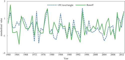
The summer runoff in the Hotan River in the period 1960–2013 had a significant correlation with the FLH (R = 0.647, the correlation coefficient passed the significance test of 0.001, P < 0.001), indicating that high atmosphere temperature variations influence runoff (Fig. 4), in agreement with the results of Zhang et al. (2010) and Chen et al. (2012). This result supports our use of summer FLH to simulate and predict summer runoff of the Hotan River.

Figure 4. Time series of summer runoff and FLH in the Hotan River from 1960 to 2013.

4.2 Nonlinear response of summer runoff to FLH based on different methods

4.2.1 Wavelet analysis

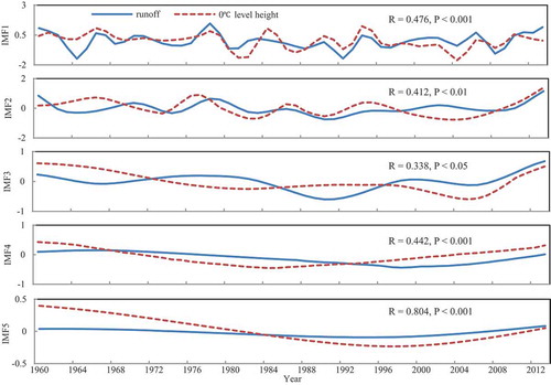
The summer runoff and FLH time series were decomposed into wavelet components at five levels (IMF1–5), corresponding to 2-, 4-, 8-, 16- and 32-year time scales (Fig. 5). Analysis of the correlation between the summer runoff and FLH at different time scales indicated that only IMF1 (R = 0.476), IMF4 (R = 0.442), and IMF5 (R = 0.804) passed the significance test of 0.001, while the correlations for IMF2 and IMF3 were less significant, passing the significance test of 0.01 (P < 0.01) and 0.05 (P < 0.05), respectively. To verify the reliability of the decomposition results, we used the summation of IMF1–5 decomposed by wavelet analysis to reconstruct runoff and FLH. The correlations between the original series and the reconstructed series for runoff (R = 0.561, P < 0.001) and FLH (R = 0.613, P < 0.001) were not high.

Figure 5. Variation patterns of summer runoff and FLH decomposed by wavelet analysis at different time scales.

4.2.2 EEMD

The EEMD produced four IMF components (IMF1–4) and one RES (Fig. 6). The IMF components indicate the fluctuations of hydrological and climatic factors at different frequencies, and the RES represents the large-scale nonlinear change over 51 years. The analysis of runoff variations in the Hotan River indicated periods of 3 and 6 years at the inter-annual scale (P < 0.05 for both, Table 1), while the analysis at the inter-decadal scale indicated periods of 11 and 22 years. The variance contribution rate of the IMF1 is the largest, reaching 66.4%.

Table 1. The period and contribution rates of EEMD decomposition for the summer runoff and FLH for the period 1960–2013 in the Hotan River. IMF: intrinsic mode function; RES: residual.

IMF component		IMF1	IMF2	IMF3	IMF4	RES
Period and significance	Runoff	3 (P < 0.05)	6 (P < 0.05)	11 (P > 0.05)	22 (P > 0.05)	-
	FLH	3 (P < 0.05)	6 (P < 0.05)	11 (P > 0.05)	23 (P > 0.05)	-
Contribution rate (%)	Runoff	66.4%	25.6%	1.8%	2.9%	3.2%
	FLH	50.5%	25.3%	20.9%	0.5%	2.8%

Figure 6. The intrinsic mode functions IMF1–4 and trend components of summer runoff and FLH from 1960 to 2013 in the Hotan River using the EEMD method.

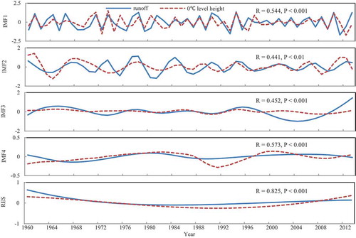
The periods of FLH are basically the same as those of runoff at the different time scales. IMF1 and IMF2 accounted for most of the variance, and had periods of 3 and 6 years (P < 0.05). This indicates that in these two components contain information that has actual physical meaning. Moreover, the EEMD results at the inter-annual and inter-decadal scales clearly illustrate the relationship between summer runoff and FLH.

Analysis of the correlations between the summer runoff and FLH at different time scales indicated that all components were significant at the 0.001 level except IMF2 (R = 0.441, P < 0.01), and the correlations of the different components were higher than those from WA. To verify the completeness and reliability of the EEMD results, we summed all components by EEMD to reconstruct the runoff and FLH values. The correlations between the reconstructed series of runoff and FLH with the original data series were up to 0.9997 (P < 0.001), indicating that this method had a good completeness and high credibility.

4.2.3 ESMD

The ESMD produced three IMF components (IMF1–3) and one RES for the summer runoff and FLH (Fig. 7). The periods of runoff were significant (P < 0.05) for 3, 6 and 14 years (Table 2), and IMF1 accounted for most of the variance (59.5%).

Table 2. The period and contribution rates of ESMD decomposition for the summer runoff and FLH for the period 1960–2013 in the Hotan River. IMF: intrinsic mode function; RES: residual.

IMF component		IMF1	IMF2	IMF3	RES
Period and significance	Runoff	3 (P < 0.05)	6 (P < 0.05)	14 (P < 0.05)	-
	FLH	3 (P < 0.05)	6 (P < 0.05)	18 (P < 0.05)	-
Contribution rate(%)	Runoff	59.5%	30.6%	3.0%	6.9%
	FLH	40.3%	19.8%	20.1%	19.8%

Figure 7. The intrinsic mode functions IMF1–3 and trend components of summer runoff and FLH from 1960 to 2013 in the Hotan River using the ESMD method.

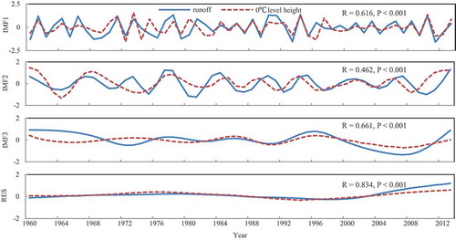
The FLH periods (3 and 6 years, P < 0.05) from ESMD at the inter-annual scale are consistent with those of runoff. However, at the inter-decadal scale, the FLH period (18 years, P < 0.05) is slightly different from those of runoff. Oscillation at the 3-year scale (IMF1) accounted for most of the inter-annual changes, indicating that this component contains most of the information with actual physical meaning.

Analysis of the correlations between summer runoff and FLH at different time scales indicated that all correlations were significant at the 0.001 level, and the correlations of the different components were greater than those from EEMD and WA. This indicates that the ESMD method better reflects the nonlinear relationships of hydroclimatic processes at different time scales. We reconstructed each component of runoff and FLH from ESMD to verify its reliability. The results indicated that all correlations between the reconstructed runoff and FLH and the original data were close to 1 (P < 0.001), thus indicating very credible results.

4.3 Simulation accuracies of different models

First, we used summer original runoff and FLH data for the period 1960–2001 with MLR and BPANN. An equation of this relationship was determined by linear regression:

$y=-0.065+0.656x$

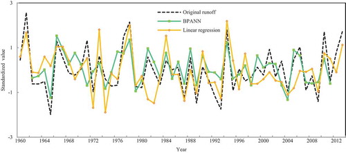
where y is the original runoff data and x is the original FLH data. The correlation between the observed runoff data with simulated values was 0.657 (P < 0.05), and the AIC was – 3.296 (Fig. 8). However, the use of the BPANN method led to a correlation between the original runoff data with the simulated series of 0.703 (P < 0.05) and an AIC of −6.139. Thus, use of the BPANN alone provided better performance than linear regression.

Figure 8. Comparison between the observed data of runoff and its simulated values based on single MLR and BPANN for calibration (1960–2001) and validation (2002–2013) periods.

We then decomposed summer runoff and FLH at different time scales using the three nonlinear decomposition methods with data from the period 1960–2001 and with hybridization to MLR or BPANN. Thus, the six hybrid models were ESMD-MLR, EEMD-MLR, WA-MLR, ESMD-BPANN, EEMD-BPANN and WA-BPANN. The calibration and validation results of different hybrid models were compared with those from MLR and BPANN alone.

For the calibration period, the multivariate linear regression equations for the summer runoff and each component of FLH decomposed by ESMD, EEMD and WA were established:

$y=-0.038+0.604a_1+0.743a_2+0.042a_3+0.364a_4$

$y=-0.005+0.711b_1+0.739b_2-0.071b_3+2.686b_4+0.829b_5$

$y=0.276+0.671c_1-0.082c_2-2.208c_3+5.438c_4-4.897c_5$

where y is the original runoff data, a_i are the four FLH components decomposed by ESMD, b_i are the five FLH components decomposed by EEMD, and c_i are the five FLH components decomposed by WA. Figure 9 shows the simulation results using the three nonlinear decomposition methods combined with MLR, for calibration and validation period. Analysis of the correlation coefficients of the validation results indicated the highest correlation between original and simulated series was for the ESMD-MLR hybrid model, followed by the EEMD-MLR hybrid model; the MLR and the WA-MLR models had the lowest correlations (Table 3). Moreover, the AIC value of the ESMD-MLR hybrid model was the lowest, followed by the EEMD-MLR hybrid model; the AIC values were highest for the MLR and WA-MLR models. The predictive QQ plot for these models (Fig. 10(a)) indicates that all four models were somewhat over-confident, particularly at the upper end of the distribution, during the calibration period. During the calibration and validation periods, the ESMD-MLR model had the highest Cronbach’s α and NSE, and the lowest RMSE, indicating higher reliability. Clearly, the hybrid model improved the simulation compared with use of MLR alone. Both hybrid models – ESMD-MLR and EEMD-MLR – had higher accuracy, and ESMD-MLR was slightly better than EEMD-MLR. However, the simulation of extreme points by these three models requires further improvement.

Table 3. Comparison between single model and hybrid models of MLR and nonlinear decomposition methods for calibration (1960–2001) and validation (2002–2013). Bold indicates the best performance.

	MLR	ESMD-MLR	EEMD-MLR	Wavelet-MLR
Calibration (1960–2001)
R	0.655 (P < 0.001)	0.752 (P < 0.001)	0.720 (P < 0.001)	0.691 (P < 0.001)
AIC	–22.670	–34.159	–29.783	–25.507
RMSE	0.745	0.650	0.685	0.721
NSE	0.429	0.566	0.518	0.466
α	0.849	0.864	0.857	0.809
Validation (2002–2013)
R	0.657 (P < 0.05)	0.735 (P < 0.01)	0.712 (P < 0.01)	0.676 (P < 0.01)
AIC	–3.296	–6.978	–5.823	–3.617
RMSE	0.802	0.688	0.722	0.791
NSE	0.343	0.517	0.468	0.361
α	0.664	0.870	0.852	0.776

Figure 9. Comparison between the observed data of runoff and its simulated values based on the hybrid models of MLR and nonlinear decomposition methods for calibration (1960–2001) and validation (2002–2013).

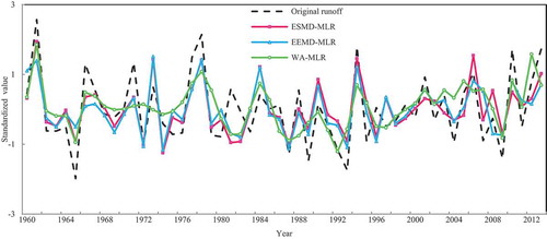
Figure 10. Predictive QQ plots obtained based on the prediction distributions generated using the single MLR and the hybrid models of MLR combined with nonlinear decomposition methods for (a) the calibration period (1960–2001) and (b) the validation period (2002–2013).

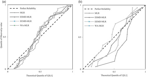
Figure 11 shows the results of hybrid prediction based on combination of three nonlinear decomposition methods with BPANN. Analysis of the correlation coefficients for the validation results (Table 4) indicates the correlation between the original and simulated series was greatest for the ESMD-BPANN hybrid model, followed by the EEMD-BPANN hybrid model. The correlations of BPANN alone and the WA-BPANN hybrid model were the lowest. Moreover, the AIC was lowest for the ESMD-BPANN hybrid model, followed by the EEMD-BPANN hybrid model; the AIC of the BPANN alone and the WA-BPANN hybrid model were the highest.

Table 4. Comparison between single model and hybrid models of BPANN and nonlinear decomposition methods for calibration (1962–2001) and validation (2002–2011). Bold indicates best performance.

	BPANN	ESMD-BPANN	EEMD-BPANN	Wavelet-BPANN
Calibration (1962–2001)
R	0.712	0.863	0.824	0.751
	(P < 0.001)	(P < 0.001)	(P < 0.001)	(P < 0.001)
AIC	–28.0927	–57.666	–50.160	–37.496
RMSE	0.686	0.474	0.521	0.610
NSE	0.438	0.732	0.676	0.556
α	0.790	0.892	0.878	0.840
π^(rel)	0.762	1.861	1.534	0.925
Validation (2002–2011)
R	0.703	0.853	0.794	0.724
	(P < 0.05)	(P < 0.001)	(P < 0.01)	(P < 0.01)
AIC	–6.139	–12.719	–7.259	–6.948
RMSE	0.666	0.479	0.562	0.639
NSE	0.471	0.726	0.577	0.512
α	0.694	0.906	0.823	0.801
π^(rel)	0.586	1.529	1.242	0.693

Figure 11. Comparison between the observed data of runoff and its simulated values based on the hybrid models of BPANN and nonlinear decomposition methods for calibration (1962–2001) and validation (2002–2011) periods.

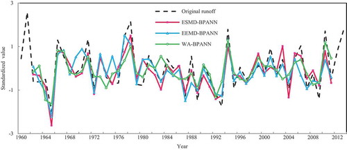
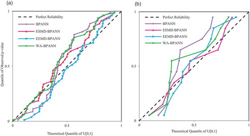
Figure 12 shows the predictive QQ plots for these models. These results show again that all four models were somewhat over-confident during the calibration and validation periods. The ESMD-BPANN model had the highest Cronbach’s α, indicating the highest reliability; this model also had the highest NSE value and the lowest RMSE value. In addition, the high π^(rel) value of the ESMD-BPANN hybrid model demonstrates good resolution of the forecast distributions. Thus, this hybrid model obviously has better simulation accuracy than BPANN alone. The ESMD-BPANN hybrid model had the highest precision, and had good reliability and resolution.

Figure 12. Predictive QQ plots obtained based on the prediction distributions generated using the single BPANN and hybrid models of BPANN combined with nonlinear decomposition methods for (a) the calibration (1962–2001) period and (b) the validation period (2002–2011).

Our comparisons of the simulation results indicated that the hybrid models based on the nonlinear methods and BPANN provided better accuracy and simulation of extreme points than hybrid models based on nonlinear methods and MLR (Tables 3 and 4). In addition, the ESMD-BPANN hybrid prediction model had the highest simulation accuracy among all tested models. Therefore, the ESMD-BPANN hybrid model should be employed to characterize the response of runoff to climate change and to predict future trends of runoff.

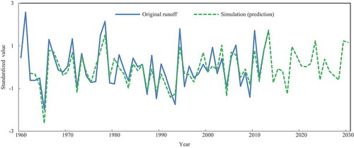
The ESMD-BPANN hybrid model exhibited the greatest accuracy among all eight models that we examined to predict runoff variations in the Hotan River from 2014–2030 (Fig. 13). Our forecasts indicate that the future runoff will have significant fluctuations, and a trend for a slight increase from 2014–2030, at a rate of 12.4 hm³/year. This model forecasted low runoff values for 2014, 2017, 2024 and 2028, and high ones for 2018, 2023, 2029 and 2030. This indicates that the inter-annual variations of runoff will be large and unstable. According to the actual data from 2014–2017, the change of runoff exhibits rising-decreasing, and the low runoff lies in 2014 and 2017, which is consistent with the predicted results. Moreover, the average error rate of the predicted and actual values from 2014–2017 is 8.66%. Therefore, hydrologists must devote further attention to variations of runoff, so they can formulate strategies for improved management of water resources.

Figure 13. Projected runoff in the Hotan River by the hybrid model ESMD-BPANN for the period 2014–2030.

5 Discussion

5.1 The advantages and disadvantages of the models

Analysis of the nonlinear decomposition results for runoff and atmospheric factors indicated that EEMD and ESMD had higher completeness than WA. Thus, the results of ESMD and EEMD are more reliable. These two methods are relatively new, and are both derived from the EMD method. In particular, for EEMD, the signal with added white noise is decomposed using EMD to obtain the means of the ensemble. As more noise is added, the noise of the average result declines, and the outputs are closer to the actual values (Wu and Huang 2009). The ESMD method achieves the adaptive global mean using a least squares method, which has strong adaptability and local characteristics. In contrast, WA is non-adaptive, and the signal is decomposed into several linear combinations to satisfy the fluctuation of an a priori basis function.

The significance analysis of runoff periods at different time scales indicated that four IMF components (IMF1–4) were obtained by EEMD for runoff and FLH, although the periods of IMF3 and IMF4 were not significant. However, the periods of three IMF components (IMF1–3) decomposed by ESMD were significant at the level of 0.05. Evidently, ESMD is superior to EEMD in reducing noise when processing decomposition results.

Our analysis of the correlation between the summer runoff and FLH at different time scales indicated that all IMF components decomposed by ESMD were significant at the level of 0.001, and the correlations of the different components were higher than from of EEMD and WA. The wavelet is predicated on a priori selection of basis functions that are either of infinite length or have fixed finite length, and may cause spurious oscillations (Ayenu-Prah and Attohokine 2009). However, EEMD has self-adaptability, and the decomposition results depend on the length of the data, not the number of decompositions. In the ESMD method, the internal extreme-point symmetric interpolation method is applied (instead of the envelop symmetric method, as in EEMD), and the optimal sifting times are determined during the decomposition. This can effectively resolve the “mode mixing” issue of EEMD (Wang and Li 2014). Accordingly, our decomposition results show that ESMD has good stability and completeness, and a better accuracy for processing nonlinear processes. Therefore, this method better reflects the nonlinearities of hydroclimatic processes at different time scales.

Admittedly, there exists uncertainty in the decomposition process of the three nonlinear methods. The choices of wavelet decomposition level, wavelet function and wavelet threshold de-noising impact the accuracy of wavelet decomposition (Sang et al. 2009, Nourani et al. 2011). Some researchers have evaluated the uncertainty of decomposition results in wavelet-based signal analysis (Peretto et al. 2005, Schafer et al. 2005, Tse and Lai 2007, Sang et al. 2018). According to the criteria of self-similarity, compactness and smoothness for wavelet selection (Ramsey 1999), Symlet 8 was chosen as the wavelet function in this research. In addition, in terms of the decomposition of EEMD, Wu and Huang (2009) indicates that increasing noise amplitudes and ensemble numbers alter the decomposition little as long as added noise has moderate amplitude and the ensemble has a large enough number of trials, and the EEMD can be used without subjective intervention, providing a sort of robustness results. To estimate the uncertainty of EEMD, the runoff data were decomposed 10 times by the EEMD method. We found that the correlation coefficients between the decomposition results were close to unit, which shows that the decomposition result of EEMD is relatively stable. Furthermore, the decomposition process of ESMD also exists uncertainty. A good sifting scheme is anticipated yielding a unique IMF with a small decomposition error. Wang and Li (2013) indicate that ESMD does not decompose the data to the residual curve with at most one extreme point, it optimizes the last trend component to be an optimal “adaptive global mean” curve which possesses a certain number of extreme points. The sifting times can be determined and the optimal decomposition is output of the optimization procedure.

Applications of physically-based hydrological models that incorporate the glacier module (Huss et al. 2010, Finger et al. 2011, Luo et al. 2013, Wang et al. 2015) are usually limited to watersheds with substantial observations. Ragettli et al. (2015) found that if no local data had been available for their estimation, the calibration approach resulted in parameter values that would have been different. Moreover, conceptual models (Engelhardt et al. 2014, Van Beusekom and Viger 2016) easily include the inherent random component that characterizes hydrological processes, leading to the prediction uncertainty is typically very high. Using conceptual model, Wang et al. (2019) indicated that in high elevation areas, where meteorological stations are absent, it is difficult to estimate the accuracy of corrected TRMM precipitation data; resulting in uncertainty sourced from precipitation lapse rates at high-altitude regions. However, the initial guess of the parameters and the sampling variability of the training patterns of ANN do not have significant impact on the model performance (Srivastav et al. 2007). Peng et al. (2017) and Nayak et al. (2013) reported that the WA-BPANN hybrid model improved the simulation of runoff. Xu et al. (2016) and He et al. (2015) showed that the accuracy of the EEMD-BPANN hybrid model was better than BPANN alone. However, the present paper demonstrated that the accuracy of the ESMD-BPANN hybrid model was significantly better than the accuracies of EEMD-BPANN, WA-BPANN, and BPANN alone. This indicates that considering the nonlinear trends of a hydroclimatic system at different time scales provides a more accurate characterization of the response of hydrological processes to climate change, and improves the accuracy of runoff simulation; it also clear that the ESMD-BPANN hybrid model had much better accuracy, and is therefore suitable for use as a new reference for runoff simulation and prediction.

5.2 Hydrological processes understanding in the study area

The runoff of the different components decomposed by ESMD had oscillation periods of 3, 6 and 14 years, consistent with the regular variations of oceanic and atmospheric events (Chen et al. 2001). In particular, the inter-annual periods of 3 and 6 years are similar to the periods of El Niño–Southern Oscillation (ENSO) events (Allan 2000), which range from 2 to 8 years, so it is possible that ENSO contributes to these runoff events. The underlying surface also affects the periodic variations of runoff. This means that changes in the hydrological series are mainly responses to external changes, depending on the conditions of the underlying surface (Yang and Li 2004). In addition, there is a 3-year period for oscillations of the location of the ridgeline of the Subtropical High, and a 7-year period for oscillations of polar migration amplitude, both of which influence precipitation in western China (Xu and Dong 1982, Chen 1995, Zhou et al. 2000, Ding et al. 2001). Changes of these two factors can alter the Earth’s centrifugal force system, and lead to changes of atmospheric circulation, air quality, and moisture transport, all of which affect hydrological systems.

Same cycle in change periodicity and similar nonlinear trends at the inter-annual scale indicates that there may be a close relationship between the runoff and FLH. The Hotan River originates from high Kunlun Mountains, and high mountains glaciers are sensitive to climate change in the context of global change (Kang et al. 2002). The ascending or decreasing of FLH will influence the fluctuation of mountainous surface 0°C line to a certain extent, which can thus influence the glacier-snow meltwater processes on high mountains (Zhang et al. 2010). The high-mountain snow and ice meltwater of the Hotan River produced approximately 56% of the annual runoff (Chen et al. 2012). However, with the changes in near-surface temperature, mean summer FLH was reduced around the abrupt change point (occurred in 1974) (Chen et al. 2012). It may be related to the surface sensible heat flux in the northwest of Qinghai-Tibet Plateau, which mainly exists to transfer energy from surface to atmosphere (Ji and Huang 2006). Different methods were used by Duan and Wu (2008) and Yang et al. (2011) to analyse the time series of surface sensible heat flux in the Qinghai-Tibet Plateau. The results indicated a strong weakening trend, especially in summer (Yang et al. 2011), which can result in the heating effect of surface weakened on the lower layer of high atmosphere. It may be the direct cause of a reduction in summer FLH. When the summer FLH was reduced, the temperature around glaciers decreased, glacial area under FL declined, glacial melt slowed down, liquid precipitation was frozen, water resource was reserved in mountain areas as glaciers, snows, etc. material accumulation increased, and the recharge of river runoff from glacial meltwater runoff reduced. Thus, under the background of global warming, no significant changes occur to summer mountain runoff of Hotan River. Moreover, Wang et al. (2008b) analysed the sensitivity of China’s glacial system to climate change using the functional model on glacial system change, indicating that the glaciers in the Kunlun Mountains belong to a stable type. It can be seen that there were slight differences in the periods of runoff and FLH in the Hotan River at the inter-decadal scale to be reasonable.

In recent years, many experts currently do not accept the concept of nonstationarity at hydroclimatic systems (Montanari and Koutsoyiannis 2012, 2015, Serinaldi and Kilsby 2015). Instead, they accept that the notions of stationarity and nonstationarity apply only to models, and not to real-world processes (Oreskes et al. 1994). When there is additional information on the cause of time-dependent behaviours, then a nonstationary model is suitable. While without this additional information, predictions based on pure data-driven time-dependent patterns may yield physically inconsistent results (Serinaldi et al. 2018). Thus, the data alone are insufficient for selection of the most appropriate nonstationary model. To claim nonstationarity, two conditions must be present: (a) deductive reasoning to establish the deterministic function of time, and (b) validation of the deterministic function by data which were not used in the model construction (Koutsoyiannis and Montanari 2015). In this paper, the different decomposition methods only conduct stationary processing for the time series, as the concepts of stationarity and nonstationarity in hydroclimatic systems remain ambiguous.

6 Conclusions

There are five major conclusions of our study.

First, the nonlinear decomposition results for runoff and FLH from ESMD and EEMD were superior to those from WA. However, the statistical significance of the periods of the different components was better for ESMD than EEMD.

Second, the results of ESMD show that runoff variance at 3 years accounted for most of the variance (59.5%). The summer runoff had an obvious response to FLH at an inter-annual scale, and both had periods of 3 years and 6 years (P < 0.05 for both). However, there were slight differences at the inter-decadal scale, in that runoff had a period of 14 years (P < 0.05) and FLH had a period of 18 years (P < 0.05). In addition, the correlation between the summer runoff and FLH had obvious differences at different time scales.

Third, the BPANN alone provided better simulation than linear regression. Moreover, hybrid models, based on three different nonlinear decomposition methods, combined with MLR further improved the simulation relative to MLR alone. The correlation between original data and simulated series was best for the ESMD-MLR hybrid model. The ESMD-MLR model also had the highest Cronbach’s α and NSE, and the lowest AIC and RMSE, indicating its high reliability.

Fourth, a hybrid model with BPANN had better accuracy than BPANN alone, and better accuracy that hybrid models based on three different nonlinear decomposition methods with MLR. Among these hybrid models, the accuracy of the ESMD-BPANN hybrid model was best in terms of reliability and resolution. Therefore, the nonlinear nature of this hydroclimatic system must be considered for accurate simulations. The ESMD-BPANN hybrid model provided the best simulation of the nonlinear response of runoff to FLH, and should be considered as a new reference for runoff prediction.

Fifth, the ESMD-BPANN hybrid model predicts that runoff in the Hotan River will increase at a rate of 12.4 hm³/year from 2014 to 2030.

A limitation of the hybrid modelling approach, however, is that an ANN is a pure data-driven prediction method, and it does not consider the possible physical meaning of a time series in the modelling process. Thus, this method can bring several uncertainties in the results (Kasiviswanathan et al. 2018). In addition, in the modelling process, only the influences of variations in summer FLH on runoff are discussed, without involving precipitation, temperature, evapotranspiration and other meteorological drivers. Furthermore, the extreme points of runoff have not been accurately simulated.

In future research, on the basis of acquiring sufficient data, a hydrological model with a clear physical basis that can truly reflect the runoff production process and the response mechanism to climate change in the basin of ARNC will be established. Moreover, further exploration is required for comprehensive influence mechanisms of all key meteorological factors on changes in runoff. Last but not least, it is important to further improve the predictions of extreme events of the examined hydrological processes.

Acknowledgements

We are grateful to the anonymous reviewers and the Associate Editor, Dr Andreas Efstratiadis, for their insightful and constructive comments that substantially improved the manuscript.

Disclosure statement

No potential conflict of interest was reported by the authors.

Additional information

Funding

This research is supported by the National Natural Science Foundation of China [41501211] and ECNU Academic Innovation Promotion Program for Excellent Doctoral Students [YBNLTS2019-003].

References

- Abrahart, R.J., et al., 2012. Two decades of anarchy? Emerging themes and outstanding challenges for neural network river forecasting. Progress in Physical Geography, 36 (4), 480–513. doi:10.1177/0309133312444943
- Ahani, A., Shourian, M., and Rad, P.R., 2017. Performance assessment of the linear, nonlinear and nonparametric data driven models in river flow forecasting. Water Resources Management, 32 (1), 1–17.
- Allan, R.J., 2000. ENSO and climatic variability in the past 150 years. El Niño and the Southern Oscillation: multi-scale variability, global and regional impacts. New York: Cambridge University Press.
- Anderson, D.R., Burnham, K.P., and Thompson, W.L., 2000. Null hypothesis testing: problems, prevalence, and an alternative. The Journal of Wildlife Management, 64 (4), 912–923. doi:10.2307/3803199
- Ayenu-Prah, A.Y. and Attohokine, N.O., 2009. Comparative study of Hilbert-Huang transform, fourier transform and wavelet transform in pavement profile analysis. Vehicle System Dynamics, 47 (4), 437–456. doi:10.1080/00423110802167466
- Bradley, R.S., et al., 2012. Recent changes in freezing level heights in the Tropics with implications for the deglacierization of high mountain regions. Geophysical Research Letters, 36 (17), 367–389.
- Chen, R.S., Kang, E.S., and Zhang, J.S., 2001. Application of wavelet transform on annual runoff, yearly average air temperature and annual precipitation periodic variations in Hexi region. Advance in Earth Sciences, 16 (3), 339–345. (in Chinese).
- Chen, X.F., 1995. The anomaly change of subtropical high and its formation cause in West Pacific. Meteorological Monthly, 21 (12), 3–7. (in Chinese).
- Chen, Y.N., et al., 2015. Progress and prospects of climate change impacts on hydrology in the arid region of northwest China. Environmental Research, 139, 11–19. doi:10.1016/j.envres.2014.12.029
- Chen, Z.S., Chen, Y.N., and Li, W.H., 2012. Response of runoff to change of atmospheric 0℃ level height in summer in arid region of Northwest China. Science China Earth Sciences, 55 (9), 1533–1544. doi:10.1007/s11430-012-4472-6
- Daliakopoulos, I.N. and Tsanis, I.K., 2016. Comparison of an artificial neural network and a conceptual rainfall–runoff model in the simulation of ephemeral streamflow. Hydrological Sciences Journal, 61 (15), 2763–2774. doi:10.1080/02626667.2016.1154151
- Ding, H.W., et al., 2001. Trend prediction and characteristics of runoff variation into the Danghe reservoir. Journal of Desert Research, 21 (z1), 38–42. (in Chinese).
- Duan, A.M. and Wu, G.X., 2008. Weakening trend in the atmospheric heat source over the Tibetan Plateau during recent decades. Part I: observations. Journal of Climate, 21, 3149–3164. doi:10.1175/2007JCLI1912.1
- Engelhardt, M., Schuler, T.V., and Andreassen, L.M., 2014. Contribution of snow and glacier melt to discharge for highly glacierised catchments in Norway. Hydrology and Earth System Sciences, 18 (18), 511–523. doi:10.5194/hess-18-511-2014
- Finger, D., et al., 2011. The value of glacier mass balance, satellite snow cover images, and hourly discharge for improving the performance of a physically based distributed hydrological model. Water Resources Research, 47, W07519. doi:10.1029/2010wr009824
- Garvelmann, J., Pohl, S., and Weiler, M., 2015. Spatio-temporal controls of snowmelt and runoff generation during rain-on-snow events in a mid-latitude mountain catchment. Hydrological Processes, 29 (17), 3649–3664. doi:10.1002/hyp.v29.17
- He, L., et al., 2015. Multi-scale prediction of regional sea level change based on EEMD and BP neural network. Quaternary Sciences, 35 (2), 374–382. (in Chinese).
- He, M.X., et al., 2011. Corruption of parameter behavior and regionalization by model and forcing data errors: a Bayesian example using the SNOW17 model. Water Resources Research, 47 (7), W07546. doi:10.1029/2010WR009753
- Hsu, K., Gupta, H.V., and Sorooshian, S., 1995. Artificial neural network modeling of the rainfall-runoff process. Water Resources Research, 31 (31), 2517–2530. doi:10.1029/95WR01955
- Hu, X.Y., et al., 2017. Variation characteristics and influence factors of potential evapotranspiration in Hotan region in recent 54 years. Research of Soil and Water Conservation, 24 (1), 145–150.
- Huang, N.E. and Wu, Z.H., 2008. A review on Hilbert–huang transform: method and its applications to geophysical studies. Reviews of Geophysics, 46 (2), 1–23. doi:10.1029/2007RG000228
- Huang, S.Z., et al., 2014. Monthly streamflow prediction using modified EMD-based support vector machine. Journal of Hydrology, 511 (7), 764–775. doi:10.1016/j.jhydrol.2014.01.062
- Huang, Y.X., et al., 2009. Analysis of daily river flow fluctuations using empirical mode decomposition and arbitrary order Hilbert spectral analysis. Journal of Hydrology, 373 (1–2), 103–111. doi:10.1016/j.jhydrol.2009.04.015
- Humphrey, G.B., et al., 2016. A hybrid approach to monthly streamflow forecasting: integrating hydrological model outputs into a Bayesian artificial neural network. Journal of Hydrology, 540, 623–640. doi:10.1016/j.jhydrol.2016.06.026
- Huss, M., et al., 2010. Modelling runoff from highly glacierized alpine drainage basins in a changing climate. Hydrological Processes, 22 (19), 3888–3902. doi:10.1002/hyp.7055
- Ji, J.J. and Huang, M., 2006. The estimation of the surface energy fluxes over Tibetan Plateau. Advances in Earth Science, 21 (12), 1268–1272.
- Kan, G.Y., et al., 2015. Improving event-based rainfall-runoff simulation using an ensemble artificial neural network based hybrid data-driven model. Stochastic Environmental Research & Risk Assessment, 29 (5), 1345–1370. doi:10.1007/s00477-015-1040-6
- Kang, E.S., Cheng, G.D., and Dong, Z.C., 2002. Glacier-snow water resources and mountain runoff in the arid area of Northwest China. Beijing: Science Press.
- Kashani, M.H., et al., 2016. Integration of Volterra model with artificial neural networks for rainfall-runoff simulation in forested catchment of northern Iran. Journal of Hydrology, 540, 340–354. doi:10.1016/j.jhydrol.2016.06.028
- Kasiviswanathan, K.S., Sudheer, K.P., and He, J., 2018. Probabilistic and ensemble simulation approaches for input uncertainty quantification of artificial neural network hydrologic models. Hydrological Sciences Journal, 63 (1), 101–113. doi:10.1080/02626667.2017.1393686
- Kermani, B.G., Schiffman, S.S., and Nagle, H.G., 2005. Performance of the Levenberg–marquardt neural network training method in electronic nose applications. Sensors & Actuators B Chemical, 110 (1), 13–22. doi:10.1016/j.snb.2005.01.008
- Kisi, O., 2010. Wavelet regression model for short-term streamflow forecasting. Journal of Hydrology, 389 (3–4), 344–353. doi:10.1016/j.jhydrol.2010.06.013
- Koutsoyiannis, D. and Montanari, A., 2015. Negligent killing of scientific concepts: the stationarity case. International Association of Scientific Hydrology Bulletin, 60 (7– 8), 1174– 1183. doi:10.1080/02626667.2014.959959
- Laio, F. and Tamea, S., 2007. Verification tools for probabilistic forecasts of continuous hydrological variables. Hydrology & Earth System Sciences, 11 (4), 1267–1277. doi:10.5194/hess-11-1267-2007
- Li, B.F., et al., 2018. Why does the runoff in Hotan River show a slight decreased trend in northwestern China? Atmospheric Science Letters, 19, 1. doi:10.1002/asl.800
- Luo, Y., et al., 2013. Inclusion of glacier processes for distributed hydrological modeling at basin scale with application to a watershed in Tianshan Mountains, northwest China. Journal of Hydrology, 477 (477), 72–85. doi:10.1016/j.jhydrol.2012.11.005
- Maier, H.R. and Dandy, G.C., 1998. The effect of internal parameters and geometry on the performance of back-propagation neural networks: an empirical study. Environmental Modelling& Software, 13 (2), 193–209. doi:10.1016/S1364-8152(98)00020-6
- Mallat, S.G., 1989. A theory for multi-resolution signal decomposition: the wavelet representation. IEEE Transactions Pattern Analysis and Machine Intelligence, 11 (7), 674–693. doi:10.1109/34.192463
- Mason, S.J. and Stephenson, D.B., 2008. How do we know whether seasonal climate forecasts are any good? Berlin: Springer.
- Modarres, R., 2008. Multi-criteria validation of artificial neural network rainfall-runoff modeling. Hydrology & Earth System Sciences, 13 (3), 411–421. doi:10.5194/hess-13-411-2009
- Moghadassi, A.R., et al., 2009. A new approach for estimation of PVT properties of pure gases based on artificial neural network model. Brazilian Journal of Chemical Engineering, 26 (1), 199–206. doi:10.1590/S0104-66322009000100019
- Montanari, A. and Koutsoyiannis, D., 2012. A blueprint for process-based modeling of uncertain hydrological systems. Water Resources Research, 48 (9), 9555. doi:10.1029/2011WR011412
- Montanari, A. and Koutsoyiannis, D., 2015. Modeling and mitigating natural hazards: stationarity is immortal! Water Resources Research, 50 (12), 9748–9756. doi:10.1002/2014WR016092
- Nayak, P.C., et al., 2013. Rainfall-runoff modeling using conceptual, data driven, and wavelet based computing approach. Journal of Hydrology, 493 (13), 57–67. doi:10.1016/j.jhydrol.2013.04.016
- Nayak, P.C., Sudheer, K.P., and Jain, S.K., 2007. Rainfall‐runoff modeling through hybrid intelligent system. Water Resources Research, 43 (W07415), 931–936. doi:10.1029/2006WR004930
- Ning, L., et al., 2016. Runoff of arid and semi-arid regions simulated and projected by CLM-DTVGM and its multi-scale fluctuations as revealed by EEMD analysis. Journal of Arid Land, 8 (4), 506–520. doi:10.1007/s40333-016-0126-4
- Nourani, V., et al., 2014. Applications of hybrid wavelet–Artificial Intelligence models in hydrology: a review. Journal of Hydrology, 514, 358–377. doi:10.1016/j.jhydrol.2014.03.057
- Nourani, V., Kisi, Ö., and Komasi, M., 2011. Two hybrid artificial intelligence approaches for modeling rainfall-runoff process. Journal of Hydrology, 402 (1–2), 41–59. doi:10.1016/j.jhydrol.2011.03.002
- Oreskes, N., Shrader-Frechette, K., and Belitz, K., 1994. Verification, validation, and confirmation of numerical models in the Earth sciences. Science, 263 (5147), 641–646. doi:10.1126/science.263.5147.641
- Peng, T., et al., 2017. Streamflow forecasting using empirical wavelet transform and artificial neural networks. Water, 9 (6), 406. doi:10.3390/w9060406
- Peretto, L., Sasdelli, R., and Tinarelli, R., 2005. On uncertainty in wavelet-based signal analysis. IEEE Transactions on Instrumentation and Measurement, 54 (4), 1593–1599. doi:10.1109/TIM.2005.851210
- Qin, Y.H., et al., 2018. Spatio-temporal variations of nonlinear trends of precipitation over an arid region of northwest China according to the extreme-point symmetric mode decomposition method. International Journal of Climatology, 38 (5), 2239–2249. doi:10.1002/joc.5330
- Ragettli, S., et al., 2015. Unraveling the hydrology of a Himalayan catchment through integration of high resolution in situ data and remote sensing with an advanced simulation model. Advances in Water Resources, 78, 94–111. doi:10.1016/j.advwatres.2015.01.013
- Ramsey, J.B., 1999. Regression over timescale decompositions: a sampling analysis of distributional properties. Economic Systems Research, 11 (2), 163–184. doi:10.1080/09535319900000012
- Renard, B., et al., 2010. Understanding predictive uncertainty in hydrologic modeling: the challenge of identifying input and structural errors. Water Resources Research, 46 (5), 1187–1191. doi:10.1029/2009WR008328
- Sang, Y.F., et al., 2009. Entropy-Based wavelet de-noising method for time series analysis. Entropy, 11 (4), 1123–1148. doi:10.3390/e11041123
- Sang, Y.F., et al., 2018. A discrete wavelet spectrum approach for identifying non-monotonic trends in hydroclimate data. Hydrology and Earth System Sciences, 22 (1), 757–766. doi:10.5194/hess-22-757-2018
- Schafer, B.M., Pfrommer, C., and Zaroubi, S., 2005. Redshift estimation of clusters by wavelet decomposition of their Sunyaev-Zel’dovich morphology. Monthly Notices of the Royal Astronomical Society, 362 (4), 1418–1434. doi:10.1111/j.1365-2966.2005.09419.x
- Serinaldi, F. and Kilsby, C.G., 2015. Stationarity is undead: uncertainty dominates the distribution of extremes. Advances in Water Resources, 77, 17–36. doi:10.1016/j.advwatres.2014.12.013
- Serinaldi, F., Kilsby, C.G., and Lombardo, F., 2018. Untenable nonstationarity: an assessment of the fitness for purpose of trend tests in hydrology. Advances in Water Resources, 111, 132–155. doi:10.1016/j.advwatres.2017.10.015
- Shi, Y.F., et al., 2007. Recent and future climate change in Northwest China. Climatic Change, 80 (3–4), 379–393. doi:10.1007/s10584-006-9121-7
- Srivastav, R.K., Sudheer, K.P., and Chaubey, I., 2007. A simplified approach to quantifying predictive and parametric uncertainty in artificial neural network hydrologic models. Water Resources Research, 43 (10), 145–151. doi:10.1029/2006WR005352
- Sudheer, K.P., et al., 2010. Artificial neural network approach for mapping contrasting tillage practices. Remote Sensing, 2 (2), 579–590. doi:10.3390/rs2020579
- Swee, E.G.T. and Elangovan, S., 1999. Applications of symlets for denoising and load forecasting. In: IEEE signal processing workshop on higher-order statistics. Caesarea, 165–169.
- Taguas, E.V., et al., 2015. Modelling the rainfall-runoff relationships in a large olive orchard catchment in Southern Spain. Water Resources Management, 29 (7), 2361–2375. doi:10.1007/s11269-015-0946-6
- Tan, Q.F., et al., 2018. An adaptive middle and long-term runoff forecast model using EEMD-ANN hybrid approach. Journal of Hydrology, 567, 767–780. doi:10.1016/j.jhydrol.2018.01.015
- Tanty, R. and Desmukh, T.S., 2015. Application of artificial neural network in hydrology – a review. International Journal of Engineering Research & Technology, 4 (6), 184–188.
- Torrence, C. and Compo, G.P., 1998. A practical guide to wavelet analysis. Bulletin of the American Meteorological Society, 79 (79), 61–78. doi:10.1175/1520-0477(1998)079<0061:APGTWA>2.0.CO;2
- Tse, N.C. and Lai, L., 2007. Wavelet-based algorithm for signal analysis. EURASIP Journal on Advances in Signal Processing, 2007 (1). doi:10.1155/2007/38916
- Van Beusekom, A.E. and Viger, R.J., 2016. A glacier runoff extension to the precipitation runoff modeling system. Journal of Geophysical Research: Earth Surface, 121 (11), 2001–2021.
- Wang, C., et al., 2017. A hybrid model to assess the impact of climate variability on streamflow for an ungauged mountainous basin. Climate Dynamics, 50 (7–8), 2829–2844. doi:10.1007/s00382-017-3775-x
- Wang, J., Li, H.Y., and Hao, X.H., 2010. Responses of snowmelt runoff to climatic change in an inland river basin, Northwestern China, over the past 50 years. Hydrology and Earth System Sciences, 14 (10), 1979–1987. doi:10.5194/hess-14-1979-2010
- Wang, J.L. and Li, Z.J., 2013. Extreme-point symmetric mode decomposition method for data analysis. Advances in Adaptive Data Analysis, 5 (3), 1137. doi:10.1142/S1793536913500155
- Wang, J.L. and Li, Z.J., 2014. The ESMD method for climate data analysis. Climate Change Research Letters, 3 (1), 1–5. (in Chinese). doi:10.12677/CCRL.2014.31001
- Wang, X., et al., 2008b. Sensitivity analysis of glacier systems to climate warming in China. Journal of Geographical Sciences, 18, 190–200. doi:10.1007/s11442-008-0190-6
- Wang, X.J., Feng, G.M., and Geng, Q.Z., 2014. Application research on combined models based on wavelet analysis in prediction of daily runoff. Journal of Natural Resources, 29 (5), 885–893. (in Chinese).
- Wang, X.L., et al., 2015. Assessing the effects of precipitation and temperature on hydrological processes in a glacier-dominated catchment. Hydrological Processes, 29 (23), 4830–4845. doi:10.1002/hyp.10538
- Wang, X.Y., et al., 2019. Understanding the discharge regime of a glacierized alpine catchment in the Tianshan Mountains using an improved HBV-D hydrological model. Global and Planetary Change, 172 (2019), 211–222. doi:10.1016/j.gloplacha.2018.09.017
- Wang, Y.L., et al., 2008a. Response of summer average discharge in the Hotan River to changes in regional 0℃ level height. Advances in Climate Change Research, 4 (3), 151–155. (in Chinese).
- Weigend, A.S. and Gershenfeld, N.A., 1994. Time series prediction: forecasting the future and understanding the past. Science, 265, 1745–1746.
- Wu, C.L., Chau, K.W., and Li, Y.S., 2009. Methods to improve neural network performance in daily flows prediction. Journal of Hydrology, 372 (1–4), 80–93. doi:10.1016/j.jhydrol.2009.03.038
- Wu, Z.H., et al., 2007. On the trend, detrending, and variability of nonlinear and nonstationary time series. Proceedings of the National Academy of Sciences of the United States of America, 104 (38), 14889–14894. doi:10.1073/pnas.0701248104
- Wu, Z.H. and Huang, N.E., 2004. A study of the characteristics of white noise using the empirical mode decomposition method. Royal Society of London Proceedings Series A, 460 (2046), 1597–1611. doi:10.1098/rspa.2003.1221
- Wu, Z.H. and Huang, N.E., 2009. Ensemble empirical mode decomposition: a noise-assisted data analysis method. Advances in Adaptive Data Analysis, 1 (1), 1–41. doi:10.1142/S1793536909000047
- Xu, G.C. and Dong, A.X., 1982. The quasi-three year period of precipitation in the west of China. Plateau Meteorology, 1 (2), 11–17. (in Chinese).
- Xu, J.H., et al., 2011. An integrated statistical approach to identify the nonlinear trend of runoff in the Hotan River and its relation with climatic factors. Stochastic Environmental Research & Risk Assessment, 25 (2), 223–233. doi:10.1007/s00477-010-0433-9
- Xu, J.H., et al., 2014. Integrating wavelet analysis and BPANN to simulate the annual runoff with regional climate change: a case study of Yarkand river, northwest China. Water Resources Management, 28 (9), 2523–2537. doi:10.1007/s11269-01s4-0625-z
- Xu, J.H., et al., 2016. A hybrid model to simulate the annual runoff of the Kaidu River in northwest China. Hydrology & Earth System Sciences, 20, 1447–1457. doi:10.5194/hess-20-1447-2016
- Yadav, A.K., et al., 2015. De-noising of ultrasound image using discrete wavelet transform by symlet wavelet and filters. In: International conference on Advances in Computing, Communications and Informatics, 10–13 August 2015, Kochi, India, 1204–1208.
- Yang, K., Guo, X.F., and Wu, B.Y., 2011. Recent trends in surface sensible heat flux on the Tibetan Plateau. Science in China Series D: Earth Sciences, 54 (1), 19–28. doi:10.1007/s11430-010-4036-6
- Yang, Z.F. and Li, C.H., 2004. Abrupt and periodic changes of the annual natural runoff in the Subregions of the Yellow River. Journal of Mountain Science, 22 (2), 140–146. (in Chinese).
- Yang, Z.N., 1991. Glacier water resources in China. Lanzhou: Gansu Science and Technology Press. (in Chinese).
- Zhang, G.X., et al., 2010. The response of annual runoff to the height change of the summertime 0°C level over Xinjiang. Journal of Geographical Sciences, 20, 833–847. doi:10.1007/s11442-010-0814-5
- Zhang, Y.S. and Guo, Y., 2011. Variability of atmospheric freezing-level height and its impact on the cryosphere in China. Annals of Glaciology, 52 (58), 81–88. doi:10.3189/172756411797252095
- Zhao, A.F., et al., 2013. Changes in 0°C isotherm height of Southwest China during 1960–2010. Acta Geographica Sinica, 68 (7), 994–1006. (in Chinese).
- Zhao, X.H., et al., 2017. An EMD-based chaotic least squares support vector machine hybrid model for annual runoff forecasting. Water, 9 (3). doi:10.3390/w9030153
- Zhao, X.H. and Chen, X., 2015. Auto regressive and ensemble empirical mode decomposition hybrid model for annual runoff forecasting. Water Resources Management, 29 (8), 2913–2926. doi:10.1007/s11269-015-0977-z
- Zhou, Y.H., et al., 2000. The earth’s rotation movement and the atmosphere, ocean activities. Chinese Science Bulletin, 45 (24), 2588–2597. (in Chinese).
- Zhu, S., et al., 2016. Streamflow estimation by support vector machine coupled with different methods of time series decomposition in the upper reaches of Yangtze River, China. Environmental Earth Sciences, 75 (6), 531. doi:10.1007/s12665-016-5337-7