Estimation of irrigation return flow on monthly time resolution using SWAT model under limited data availability

ABSTRACT

This study is an assessment of the return flow ratio of an irrigation abstraction using the flow records of a downstream stream-gauging station, with the example of the Kozluk scheme irrigated by diverted water from Garzan Creek flowing through the southeastern region of Turkey. In the planning reports of the major dam projects of the region, an unverified return ratio was assumed in eliminating the influence of this irrigation on the flow measurements of Garzan Creek. The correctness of this assumed return ratio is evaluated by analysing the monthly streamflow measurements of the Besiri station through a Soil and Water Assessment Tool (SWAT) model constructed with the coarse-scale topography, land use and soil data from open source databases. The results show the necessity of irrigation project-based return flow analyses using regional fine-scale datasets, instead of rule-of-thumb assumptions, to determine the effects of irrigation activities on flow regimes more accurately.

KEYWORDS:

• irrigated agriculture
• irrigation return flow
• SWAT
• SWAT-CUP
• watershed modelling
• Garzan Basin

Editor Castellarin; Associate editor S. Kanae

1 Introduction

The most important criterion in the planning, design and operation phases of a water resources project is the basin water potential of the project site. Generally, to investigate the inflow potential of a dam project (i.e. the amounts of streamflow that the catchment above the dam site produces in response to precipitation and snow), the flow records of representative stream-gauging stations located in or near the project catchment area are utilized. In an inflow potential analysis, prior to the use of these historical measurements, the raw flow data are corrected due to the past and existing upstream water abstractions for irrigation, industry, drinking water as well as other purposes. Then, the naturalized flow values of different stations are correlated to produce the longest possible representative inflow dataset for the operational lifetime of the project. A realistic analysis of inflow potential plays a significant role to make accurate decisions on the project feasibility, on the optimum design of dam components and on the determination of operational rules in terms of the volume and timing of water releases.

For such an analysis, an important uncertainty source is in the estimate of the river-return ratio of upstream irrigation abstractions to be used in eliminating the effects of upstream irrigation schemes on the flow records of stream-gauging stations. Return flow, i.e. the portion of applied water that is not consumptively used and returns to streams from irrigated farmlands, can vary depending on irrigation and catchment characteristics such as crop type, irrigation method, land slope, soil structure and land use. Return flow fraction of water withdrawal for an upstream irrigation system is usually estimated by thumb rules depending upon site-specific conditions in terms of command area conditions and soil properties (Mohan and Vijayalakshmi 2009). For example, the use of 15–25%, 10–20% and 15–20% rates were reported for return flow fractions as the general practice in Iran, India and Turkey, respectively (Jafari et al. 2012, Gosain et al. 2005, Yalcin and Tigrek 2019). However, Gosain et al. (2005) showed that real return flow amounts can appreciably differ from usual rule-of-thumb values. Hence, it is not appropriate to set down a rule-of-thumb value that is not based on any measurements or experiments but chosen to facilitate straightforward analyses of inflow potential.

Estimation of this ratio is usually a difficult task due to the need for complex flow modelling at the scale of one or more experimental fields or at the watershed scale (Dewandel et al. 2008). Such studies require exhaustive field investigations to obtain numerous modelling data, such as pressure head profiles, water content profiles, soil characteristics, hydraulic conductivities, irrigated crops, farming practices and climatic measurements (Singh et al. 2001, Chen and Liu 2002, Chen et al. 2002, Jalota and Arora 2002). Even if the estimated rate of return is accurately assessed at the scale of the experiment, it may not be representative at the watershed scale. Moreover, the number of samples collected for the watershed-scale studies is usually limited due to time and cost issues. Hence, an accurate estimation of irrigation return flow may not be possible for large watersheds where irrigation and basin characteristics widely vary (Dewandel et al. 2008).

Gosain et al. (2005) used Soil and Water Assessment Tool (SWAT) model (Neitsch et al. 2011, Arnold et al. 2013) to predict the net water usage in the irrigated area by simulating the domain with and without utilizing the water flowing through the irrigation canal and the difference between the actual quantity of water supply and the predicted utilization of water by the developed SWAT model was treated as the return flow amount. Although the temporal variation of return flow was captured and validated by Gosain et al. (2005), the problem of hydrological modelling with SWAT is the requirement of detailed information about surface topography, soil properties, land use, weather and agricultural practices in the watershed to be analysed (Arnold et al. 2013). Data scarcity especially on the fine-scale regional soil and land use maps forces SWAT modellers to collect and analyse the required enormous data within the contexts of their studies (Ozcan et al. 2016). Another factor that constrains the application of the methodology in Gosain et al. (2005) is the presence of the required data on the actual quantities of water supply.

The objective of this study is to analyse the return flow ratio of an irrigation abstraction if the only proper data in hand is the monthly flow records of a downstream stream-gauging station, with the example of the Kozluk scheme irrigated by diverted water from Garzan Creek. Garzan Creek is one of the main tributaries of the Tigris River and its flows are measured at the Besiri stream-gauging station located at just downstream of the Kozluk irrigation area for a long time covering the period before and after the commissioning of this irrigation scheme. In the planning reports of the major dam projects located at the downstream of the Kozluk scheme, an unverified return ratio of 20% was assumed in eliminating the influence of this irrigation on the flow measurements of Garzan Creek (Ilisu Hydropower Consultants 1983, Ilisu Environment Group 2005, Enersu 2008). The correctness of this assumed return ratio is evaluated, similar to the approach in Gosain et al. (2005), by comparing the monthly streamflow estimates at the Besiri station location obtained through a SWAT model with and without introducing the agricultural activities in the irrigated area. The data scarcity problem is handled with the use of coarse-scale topography, land use and soil data from open source databases in the SWAT model development. Unlike the reference approach, the estimated quantities of water supply provided by the SWAT model are used instead of the actual amounts. In addition, due to the limited knowledge on the agricultural practices in the scheme, the uncertainty in the spatial distribution of the crop pattern is mapped onto the range of return rates by considering different irrigation scenarios.

2 Materials and methods

2.1 Study area

The Tigris is the second-longest river in western Asia after the Euphrates. It originates in eastern Turkey near Lake Hazar, about 26 km southeast of the city of Elazig, and is fed by several tributaries along its flow path through the southeastern part of Turkey before entering Iraq. The main tributaries of the upper Tigris River within the boundaries of Turkey are Garzan, Bitlis, Botan and Batman Creeks. When the planning reports of major dam projects for hydropower and irrigation purposes in the upper Tigris Basin are examined, it is seen that the river-return ratio was assumed as 20% for all existing and planned irrigation schemes (Ilisu Hydropower Consultants 1983, Ilisu Environment Group 2005, Enersu (Enersu Engineering Consultancy Construction Industry and Trade Limited Company) 2008). The only exception is the Batman-Silvan Project, for which this ratio was presumed as 15% (Suis and Sial 2001). Although the planned dominant crop types and subbasin characteristics vary from scheme to scheme or even region to region for the same scheme in such a large basin, the use of such unverified ratios for these irrigation schemes that cover an area of approximately 0.5 million hectares can cause the irrigation and hydropower potentials of the upper Tigris projects not to be used accurately (Yalcin and Tigrek 2019).

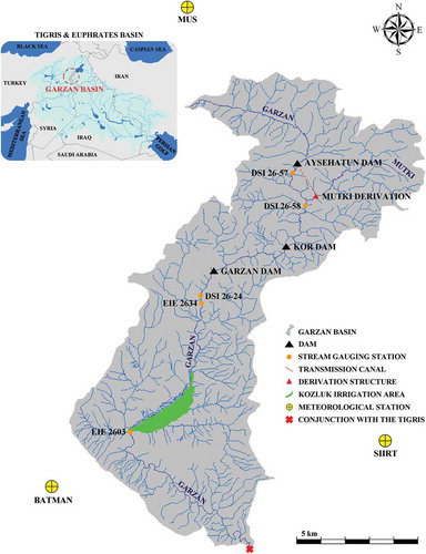
It is planned to use the water of Garzan Creek for irrigation and energy production by controlling its irregular flow regime with three dam projects. In this subbasin of the Tigris River (2912 km²), the planned hydro-system consists of the Aysehatun Dam and HEPP Project with the Mutki Derivation, the Kor Dam and HEPP Project, the Garzan Dam and HEPP Project, several run-of-river type small hydropower projects and the Garzan irrigation scheme, which covers an area of 60000 ha, as depicted in Fig. 1. Currently, only the Garzan Dam is operational since 2015 and a gross area of 3973 ha in the Garzan irrigation plan has been irrigated since 1996 under the name of the Kozluk irrigation (Yalcin and Tigrek 2019).

Figure 1. Location map of the study area.

In the low-lying parts of the Garzan Basin, the agricultural product pattern is heavily based on rain-fed crops. After the commissioning of the Kozluk irrigation, the product pattern has changed from dry farming to irrigated farming. The dominant crop types are lentil, cotton and tobacco in this irrigated area (Enersu 2008). According to the research conducted by Ilhan and Utku (2000) within a model using the Penman-Monteith method, the plant water consumptions are estimated specifically for this basin as 960.4, 909.6 and 945.0 mm/year for lentil, cotton and tobacco, respectively. In addition, the crop irrigation requirements are determined in turn as 781.4, 768.1 and 795.2 mm/year by subtracting the monthly effective rainfall and humidity from winter season rates from the monthly plant water consumption estimates (Ilhan and Utku 2000).

There are five stream-gauging stations on Garzan Creek and its tributaries, as presented in Fig. 1. As can be seen in Table 1, the only station having continuous long-period flow records and located at a more downstream altitude than the Kozluk irrigation area is the Besiri station. This situation prevents to conduct a multi-site calibration process of the basin-scale hydrologic model to be produced. However, the available monthly flow data for the period from 1981 to 1999 is sufficient for this study to analyse the effects of the existing Kozluk irrigation on the streamflow rates of the Besiri station.

Table 1. Characteristics of the stream-gauging stations.

Station ID	Station name	Opening date	Closing date	Number of years with data	Drainage area (km^2)	Elevation (m)	Mean discharge(m^3/s)
DSI 26-57	Keyburan Brook Bogazonu	24.10.1981	-	5	425.0	1200	8.6
DSI 26-58	Garzan Creek Meydanonu	29.11.1981	08.01.1999	3	783.2	909	15.8
DSI 26-24	Pisyar Creek Kozluk	01.08.1970	-	14	1359.3	620	26.0
EIE 2634	Garzan Creek Kozluk	19.10.1999	30.09.2000	1	1407.7	630	23.0
EIE 2603	Garzan Creek Besiri	01.11.1945	30.09.2000	54	2450.4	545	49.0

Sources: DSI (2007), EIE (2003).

2.2 Applied methodology

The effects of the Kozluk irrigation on the monthly flow rates at the Besiri stream-gauging station location are analysed through a SWAT model developed with the coarse-scale topography, land use and soil data from open source databases and the daily weather records of the nearby meteorological stations by simulating the flows of the Besiri station with and without introducing the agricultural activities in the irrigated area. Due to the limited knowledge on the spatial distribution of the crop pattern in the Kozluk scheme and its change through the irrigation period, four different irrigation scenarios are considered to map the uncertainty of crop pattern onto the range of return rates. The first scenario (Scenario I) corresponds to a realistic crop pattern distribution involving cotton, lentil and tobacco cultivations according to the general information available in Enersu (2008). The other scenarios are three separate cases where the same crops are practiced across the whole irrigation area (Scenario II: all cotton, Scenario III: all lentil and Scenario IV: all tobacco). The flowchart of the methodology used in this study is depicted in Fig. 2.

Figure 2. Schematic representation of the applied methodology.

The available monthly flow data of the Besiri station covering the period before and after the year 1996, the commissioning date of the Kozluk irrigation, is divided into calibration, validation and prediction sets. Firstly, the measured streamflow data of the Besiri station for the period from January 1981 to December 1990 is used to calibrate the developed SWAT model and the calibrated model is validated for the period from January 1991 to December 1995. Following the validation of the streamflow estimates of the calibrated model for the Besiri station, the model is used to simulate the natural flows at the station location ($Q_{\mathrm{s}\mathrm{i}\mathrm{m}\mathrm{u}\mathrm{l}\mathrm{a}\mathrm{t}\mathrm{e}\mathrm{d}}^{\mathrm{w}\mathrm{i}\mathrm{t}\mathrm{h}\mathrm{o}\mathrm{u}\mathrm{t}\mathrm{i}\mathrm{r}\mathrm{r}\mathrm{i}\mathrm{g}\mathrm{a}\mathrm{t}\mathrm{i}\mathrm{o}\mathrm{n}}$) between January 1996 to December 1999 (i.e. the period through which the Kozluk irrigation scheme was operational). Since the actual monthly flow amounts diverted from Garzan creek for irrigation purpose are not known, the flow records observed through the prediction period of January 1996 to December 1999 cannot be utilized directly by comparing them with the simulated natural streamflow rates of the station. Hence, to make an evaluation on the same base with the natural streamflow estimates, the agricultural activities considered in each cultivation scenario are introduced to the model separately and new simulations are performed for the prediction period to estimate the flows at the Besiri station location under the effects of the upstream agricultural activities ($Q_{\mathrm{s}\mathrm{i}\mathrm{m}\mathrm{u}\mathrm{l}\mathrm{a}\mathrm{t}\mathrm{e}\mathrm{d}}^{\mathrm{w}\mathrm{i}\mathrm{t}\mathrm{h}\mathrm{i}\mathrm{r}\mathrm{r}\mathrm{i}\mathrm{g}\mathrm{a}\mathrm{t}\mathrm{i}\mathrm{o}\mathrm{n}}$). In these simulations, the SWAT model estimates also the monthly amounts of water supply diverted to the irrigation area ($Q_{\mathrm{w}\mathrm{a}\mathrm{t}\mathrm{e}\mathrm{r}\mathrm{s}\mathrm{u}\mathrm{p}\mathrm{p}\mathrm{l}\mathrm{y}}$).

The difference between the monthly mean of the natural streamflow estimates and the corresponding monthly mean of the simulated flow values in the presence of irrigation is calculated for each month. These differences equal to the monthly net water usages in the considered cultivation scenarios ($Q_{\mathrm{n}\mathrm{e}\mathrm{t}\mathrm{u}\mathrm{s}\mathrm{a}\mathrm{g}\mathrm{e}}$). The difference between the monthly amount of water supply diverted to the irrigation area and the corresponding monthly net water usage provides how much of the diverted water from the creek is returned to the streambed in each month ($Q_{\mathrm{r}\mathrm{e}\mathrm{t}\mathrm{u}\mathrm{r}\mathrm{n}\mathrm{f}\mathrm{r}\mathrm{o}\mathrm{m}\mathrm{i}\mathrm{r}\mathrm{r}\mathrm{i}\mathrm{g}\mathrm{a}\mathrm{t}\mathrm{i}\mathrm{o}\mathrm{n}}$). The comparison of the return flows obtained under different cultivation scenarios provide the admissible ranges of return rate on monthly and annual bases.

2.3 SWAT model set-up

Three main categories of data required to construct the SWAT model are digital elevation model (DEM), soil map and land use/land cover (LULC) map. Void filled digital terrain elevation data at 1 arc-second resolution (approximately 30 m) is obtained from the global coverage public domain database of the Shuttle Radar Data Topography Mission (SRTM) (USGS 2014). The soil properties of the basin are extracted from the Digital Soil Map of the World (DSMW) version 3.6 at scale 1:5 million (FAO 2007). The LULC map is achieved from the Global Land Cover 2000 (GLC2000) version 2.0 dataset at 1 km spatial resolution (EC-JRC 2006) and it is reclassified according to the SWAT model input requirements. The other primary dataset needed in model construction is the daily weather observations of representative meteorological stations inside or near the basin to be analysed. In this context, the daily weather records of the Batman, Mus and Siirt meteorological stations on precipitation, maximum and minimum air temperature, relative humidity and wind speed for the analyse period from 1 January 1979 to 31 December 1999 including two years of model warm-up period (1979–1980) are obtained from the Turkish State Meteorological Service (MGM 2018a), whereas solar radiation is simulated using the weather generator within SWAT due to the absence of nearby stations recording this data during the analysed period (Fig. 1).

The development of the SWAT model commences with watershed delineation accomplished using the inputted DEM data (Fig. 3(a)). Streams and subbasin outlets are automatically defined utilizing the threshold method through the DEM-based stream definition option. After stream preprocessing, a new subbasin outlet is added manually at the location of the Besiri station and this outlet is selected as the whole watershed outlet to define the boundary of the study basin. Eventually, 71 subbasins are delineated for the catchment of the Besiri station, covering an area of 2450.4 km², and the watershed delineation process is completed with the calculation of subbasin parameters, such as slope gradient and slope length of the terrain (Fig. 3(b)).

Figure 3. Model development steps: (a) DEM, (b) watershed delineation, (c) land use classes, (d) soil types and (e) slope classes.

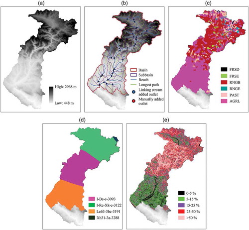
In the second step of the model construction, these subbasins are subdivided into hydrologic response units (HRUs) having unique combinations of land use, soil and topographic slope characteristics. Initially, the LULC map in the same projection with the utilized DEM data is inputted into the model in a grid format and the categories specified in the GLC2000 database are reclassified into six land use classes corresponding to the definitions of the same or similar units in the SWAT global database (Arnold et al. 2013). These classes are forest-deciduous (FRSD), forest-evergreen (FRSE), range-brush (RNGB), range-grasses (RNGE), pasture (PAST) and agricultural land-generic (AGRL), as seen in Fig. 3(c). Then, the grid-based soil data extracted from the DSMW database is uploaded into the model in the same projection with the previously inputted DEM and LULC data after updating the default “usersoil” table, which contains Unites States soils only, in the SWAT2012.mdb database file of the model according to the attributes of the DSMW soils. The resultant soil layer classified in four different soil types is presented in Fig. 3(d). Next, the slope discretization operation is applied by the multiple slope option considering five slope classes, as demonstrated in Fig. 3(e). After completing the land use, soil and slope classification procedures, percentage threshold values of 5%, 5% and 15% are set for land use, soil and slope, respectively, to eliminate minor units in each subbasin. Accordingly, a total of 572 HRUs are generated for the predefined 71 subbasins.

The third step of the model construction is the introduction of the meteorological data. The required daily weather data by SWAT model includes precipitation (mm), maximum and minimum air temperature (°C), solar radiation (MJ/m²), wind speed (m/s) and relative humidity. The default SWAT database includes only weather stations from the USA. Therefore, before importing the daily inputs into the model, the monthly weather statistics and geographic positions (in terms of latitude, longitude and elevation) of the Mus, Batman and Siirt meteorological stations are introduced to the model by updating the default “WGEN_user” table in the SWAT2012.mdb database file according to the descriptions in the “wgnrgn” table of the same database. These statistics are used by the weather generator within SWAT to simulate representative daily values for missing variables or to fill gaps in the measured data. The statistical parameters of the utilized local meteorological stations are calculated with the WGNmaker4.1.xlsm Microsoft Excel macro (Boisrame 2011), except the ones based on solar radiation, half-hour rainfall and dew point temperature data. Since these stations do not have solar radiation records during the analysed period, the required monthly mean daily solar radiation rates are derived from the long-term monthly averages of each station (MGM 2018b). The monthly maximum half-hour rainfall magnitudes are determined directly by multiplying the monthly maximum daily precipitation records with the half-hour pluviograph coefficients of each station (MGM 2018c). To estimate the average daily dew point temperature of each month over the analysed period, the DOS-based dew02.exe program (Liersch 2003) is run with the inputted maximum and minimum air temperature and percent relative humidity data for each station separately. The rainfall, temperature, wind speed and relative humidity data of the utilized stations are given to the model by the gauge location tables containing the names of the individual weather data files and the simulation of solar radiation data is left to the weather generator tool of the software.

The last step of the model construction is the configuration of simulation settings. The simulation period for an initial model run is set to be from 1 January 1979 to 31 December 1995 according to the available streamflow data of the Besiri stream-gauging station measured before the commissioning date of the Kozluk irrigation. The first two years is designated as the warm-up time of the model during which statistics are not gathered and the streamflows within the study basin are simulated on a monthly basis for a 15-year period. After this initial model simulation, the next steps are model calibration and validation processes.

2.4 Model calibration, validation and predictions

The calibration and validation analysis of the developed SWAT model is performed in the SWAT Calibration and Uncertainty Procedures (SWAT-CUP) software package (Abbaspour 2015). For model calibration, validation, sensitivity and uncertainty analysis, the Sequential Uncertainty Fitting Version 2 (SUFI-2) algorithm (Abbaspour et al. 2004, 2007) is chosen from the five different optimization procedures, namely SUFI-2, GLUE, ParaSol, McMc and PSO, provided in the SWAT-CUP package (Abbaspour 2015). In the SUFI-2 algorithm, all uncertainties, i.e. input data, model parameters, theoretical model and observed data, are mapped onto the parameter ranges and the aim is to capture most of the observed data within the 95% prediction uncertainty (95PPU) of the model in an iterative process. The 95PPU is determined at the 2.5% and 97.5% levels of the cumulative distribution of an output variable generated by the propagation of the parameter ranges (or uncertainties) using Latin hypercube sampling (Abbaspour et al. 2015). In order to attain the best range for each parameter in concern, not only the 95PPU band has to bracket most of the observed data but also the thickness of the band has to be as small as possible. Hence, the goodness of fit is assessed by the P factor and R factor (Abbaspour et al. 2004). While the P factor is the fraction of the observed data enveloped by the 95PPU band and varies from 0 to 1, the R factor is the ratio of the average thickness of the 95PPU band to the standard deviation of the observed data showing the degree of uncertainty. A P factor of 1 and an R factor of 0 indicate an ideal model simulation in which the predictions exactly corresponds to the observed data. Since a larger P factor can only be achieved with a larger R factor, a balance must be established between two indices (Abbaspour et al. 2015). Therefore, starting from initially large parameter ranges, SUFI-2 is iterated a few times by narrowing these ranges in accordance with the objective function value at each time until an optimum parameter set is reached. SUFI-2 provides eleven different objective functions, such as coefficient of determination (r²), Nash-Sutcliffe Efficiency (NSE) and mean square error (MSE). In this study, function br², defined as coefficient of determination (r²) multiplied by the slope of the linear regression line (b) between the measured and simulated variables forcing the intercept to be equal to zero, is used to account for the discrepancy in the magnitude (depicted by b) and dynamics (depicted by r²) of the observed flows and their corresponding estimates (Glavan and Pintar 2012).

After importing the text input and output files of the initial model simulation residing in the TxtInOut directory of the SWAT project to the SWAT-CUP project directory, the preliminary transaction for model calibration is adding elevation bands to the subbasin (.sub) files in order to account for elevation-dependent precipitation and temperature variations in each subbasin and, hence, to simulate snowpack and snowmelt separately for each elevation band (Abbaspour et al. 2015). For this addition, differences between the minimum and maximum elevations are calculated firstly for each subbasin and five elevation bands are considered for all subbasins except the ones where the elevation difference is too small to account for orographic effects on both precipitation and temperature. Then, mid-point elevations (ELEVB) and subbasin area fractions within the elevation bands (ELEVB_FR) are determined by using the DOS-based stand-alone Make_ELEV_BAND program located in the SWAT-CUP installation directory (Abbaspour 2015). To simulate snow cover or snowmelt at each elevation band, the values of 10 mm/km and −6°C/km are taken as an initial guess for precipitation (PLAPS) and temperature (TLAPS) lapse rates, respectively. Before starting to the model calibration process, the imported subbasin files in the SWAT-CUP project directory are updated with the elevation band data and assigned lapse rates and a single run is performed for the calibration period from January 1981 to December 1990 without changing any other parameters. Since the results are not drastically different from the records of the Besiri station, this model is referred as the default model to be calibrated (Abbaspour et al. 2015).

Model calibration consists of three main steps: (1) calibration of precipitation and temperature lapse rates and fixing them to their best simulation values, (2) calibration of sensitive snow-related parameters and fixing them to their best simulation values and (3) calibration of other sensitive modelling parameters. To avoid parameter interaction and identifiability problems, the location-specific parameters affecting evapotranspiration, precipitation and snowmelt/snow-formation processes are fitted separately and their values are fixed before adjusting other parameters for a better match with the observed streamflow data. At each step of the calibration process, the sensitivity of each parameter is evaluated firstly through a partially large parameter uncertainty range by keeping constant all other parameters at their default values. A single iteration composed of 50 simulations within the assigned parameter range is performed for the one-at-a-time analysis of each parameter. Based on the sensitive parameters and their initial ranges identified in these analyses, a combined iteration with 500 simulations is performed. At the end of this run, the software suggests new parameter ranges for another iteration focusing on the optimal parameter set that leads to the best simulation (i.e. the simulation with the best value of the objective function) of the current iteration. After adjusting the suggested parameter ranges according to the absolute parameter ranges of SWAT and previously conducted sensitivity analyses, another combined iteration is executed. These iterations are continued until no further improvements are seen in streamflow estimates in terms of the P factor, R factor and objective function (Abbaspour et al. 2004, 2007, 2015).

At the end of the first and second steps of the calibration process, the lapse rate and snow parameters are fixed in the SWAT-CUP project directory to the parameter values of the best simulation of the last iteration and taken out of the calibration process in turn. Before going to the third step, a single run is performed with the adjusted lapse rate and snow parameters to identify relevant parameters in the HRU level groundwater (.gw), soil (.sol), hydrologic response unit (.hru) and management (.mgt), the subbasin level main channel (.rte) and the watershed level basin (.bsn) input files (Abbaspour et al. 2015). Then, the one-at-a-time sensitivity analyses of the identified parameters are made following the procedure as described above. Once the model is parameterized and initial ranges are assigned, combined iterations composed of 500 simulations each are repeated until satisfactory results are obtained. Accordingly, the final iteration has the best ranges for the parameters in concern and the best simulation of the final iteration provides the best-performing parameter set.

For calibration of streamflow, a P factor value greater than 0.7 and an R factor value less than 1.5 (around 1) would be adequate depending on the model scale and the quality of the data used in constructing and calibrating the model (Abbaspour et al. 2004, 2007, 2015). According to Schuol et al. (2008) and Faramarzi et al. (2013), br² should be greater than 0.6 to be sufficient. Meanwhile, in addition to the objective function br², NSE, percent bias (PBIAS) and ratio of the root mean square error to the standard deviation of measured data (RSR) statistics are also taken into consideration to assess the calibrated model performance in terms of the best simulation. According to Moriasi et al. (2007), an NSE value between 0.75 and 1.00, a PBIAS value less than ± 10% and an RSR value less than 0.50 allow to say that the model is very good for streamflow estimates in a monthly timescale. In general, model performance can be judged as satisfactory if an NSE value higher than 0.5, a PBIAS value less than ± 25% and an RSR value less than 0.70 are obtained at the end of a monthly streamflow calibration (Moriasi et al. 2007).

After calibrating the model for the 1981–1990 period, the model is validated against the measurements of the Besiri station for the period from January 1991 to December 1995 by running a combined iteration with 500 simulations using the calibrated parameter ranges. The model performance in the validation stage is evaluated again in terms of the statistics of P factor, R factor, br², NSE, PBIAS and RSR. Following to the validation of the streamflow outputs of the calibrated model against the corresponding measurements, the natural monthly flow rates at the Besiri station location are predicted for the period from January 1996 to December 1999. A combined iteration composed of 500 simulations within the calibrated parameter ranges provides the 95PPU band of the simulated flows and the best simulation estimates are obtained by performing a single run with the best-performing parameter set attained in the model calibration stage (Lemann et al. 2017).

2.5 Streamflow predictions under the effects of the Kozluk irrigation

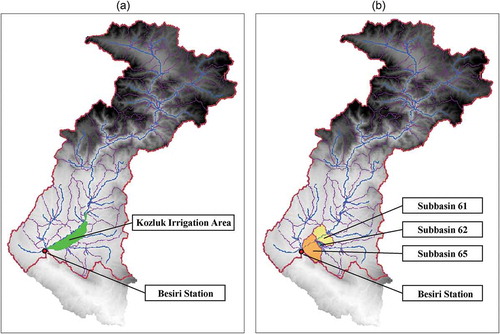
The effects of the Kozluk irrigation scheme on the streamflow rates of the Besiri station are assessed through (1) comparison of the model predictions (i.e. best simulation estimates) obtained with and without introducing the upstream agricultural activities for the best-performing parameter set and (2) comparison of the simulated results at the 50% uncertainty level (M95PPU) obtained with and without introducing the agricultural irrigation activities for the calibrated parameter ranges. To perform these comparisons, the project database file of the generated SWAT model is firstly updated with the best-performing values of all calibrated parameters including the elevation band data and the agricultural activities carried out in the Kozluk scheme is introduced to the model by editing the management data at HRU level. Subbasins 62 and 65 are selected as defining the location of the Kozluk scheme (Fig. 4). While the gross irrigated area of the scheme is 39.73 km², the total area of these two subbasins is 39.90 km², which is only about 0.43% more than the actual one. Subbasins 62 and 65 has two HRUs, namely HRU 544–545 and HRU 551–552, respectively. The land use, soil and topographic slope characteristics of these HRUs are listed in Table 2. As stated before, four different scenarios are considered including a combined case where lentil, cotton and tobacco are cultivated at the same time in the irrigation area and three separate cases where these crops are practiced across the whole irrigated land. For the combined cultivation scenario, HRU 551, HRU 552 and HRU 544–545 are designated for lentil, cotton and tobacco planting, respectively, according to the general information in Enersu (2008) (Table 2).

Table 2. Characteristics of the HRUs selected for defining the location of the Kozluk scheme.

Subbasin	HRU	Land-use class	Soil type	Slope class(%)	Area(km^2)	Cultivation scenarios for the Kozluk irrigation
						Scenario I	Scenario II	Scenario III	Scenario IV
62	544	AGRL	Lc63-3bc-3191	5–15	1.37	Tobacco	Cotton	Lentil	Tobacco
62	545	AGRL	Lc63-3bc-3191	0–5	1.79	Tobacco	Cotton	Lentil	Tobacco
65	551	AGRL	Lc63-3bc-3191	5–15	22.04	Lentil	Cotton	Lentil	Tobacco
65	552	AGRL	Lc63-3bc-3191	0–5	14.70	Cotton	Cotton	Lentil	Tobacco

Figure 4. Kozluk irrigation area: (a) actual location and (b) locations of the HRUs representing the irrigation area in the SWAT model.

The management activities are defined separately for each cultivation scenario by adjusting the general parameters on irrigation management and describing the management operations in terms of planting/beginning of growing season, auto-irrigation initialization and harvest and kill operation. In defining the irrigation management parameters in the “mgt1” table of the project database file, reach option is selected as the source of the irrigation water and the location of this source is defined as subbasin 61, positioned just upstream of the subbasins 62 and 65 (Fig. 4). In addition, minimum in-stream flow for irrigation diversions (FLOWMIN), maximum daily irrigation diversion from the reach (DIVMAX) and fraction of available flow that is allowed to be applied to the selected HRUs (FLOWFR) are set to be 0 m³/s, 150 mm and 1, respectively. The management operations defined in the “mgt2” table of the project database file are scheduled by date with one-year of rotation. The dates on which the planting/beginning of growing season and harvest and kill operations are taken from Ilhan and Utku (2000). Since tobacco is transplanted rather than established from seeds as cotton and lentil, initial leaf area index (LAI_INIT) for this plant is assigned as 0.25. Rather than specifying fixed amounts and time for irrigation, auto-application of irrigation water to be triggered by plant water demand is preferred. Auto-irrigation operations within the managed HRUs are initiated on the day after the date of planting/beginning of growing season. Auto-irrigation source code (IRR_SCA) and source location (IRR_NOA) is defined as the reach in subbasin 61. Water stress threshold that triggers irrigation (AUTO_WSTRS) is set to 0.90 for all crop types (Arnold et al. 2013). Maximum amount of water that can be applied each time when auto-irrigation is triggered (IRR_MX) is set to 10 mm. Irrigation efficiency factor (IRR_EFF) accounts for water conveyance losses and it is set to 0.90 considering a 10% loss of water in transit from the source of supply to the point of service. Surface runoff ratio (IRR_ASQ) is the fraction of applied water that is converted to runoff. This parameter is adjusted to a value of 0.30 to take into account water application losses by assuming the system farm efficiency as 0.70. Thus, the overall irrigation efficiency of the Kozluk scheme, which is equal to the multiplication of the water conveyance and water application efficiencies, is considered as 0.63.

In addition, SWAT utilizes two heat unit indexes in the management operations, namely total base zero heat units (PHU₀) and total heat units required for a plant to reach maturity (PHU). PHU₀ is the summation of mean daily air temperatures for an entire year and PHU equals to the summation of mean daily air temperatures above the plant’s base or minimum temperature for growth starting from the date of planting until the day it reaches maturity. Although PHU₀ is calculated by SWAT using the long-term weather data provided in the “wgn” table of the project database file, plant PHU must be inputted (Neitsch et al. 2011). Total head units required to bring the crops of the Kozluk scheme to maturity are firstly calculated via the DOS-based potential head unit program (SWAT-PHU 2017) using the long-term mean monthly maximum and minimum temperature data of the closest weather station (i.e. Batman) (MGM 2018a), the latitude of the irrigation area, the base or minimum temperatures required by the plants for growth (Arnold et al. 2013) and the average number of days for the plants to reach maturity (Ilhan and Utku 2000). However, the accuracy of the determined plant PHUs should be checked due to their direct effects on the simulation results. The model simulates plant growth until the crop reaches maturity and from that point on, it does not transpire or take up water (Neitsch et al. 2011). Therefore, the control is made by means of the fractions of PHU₀ and PHU obtained by performing a trial model simulation for the 1996–1999 period. A PHU₀ fraction of 0.15 has been found to provide reasonable timings for planting operations and PHU fractions of 1.0 and 1.2 are advised to conduct harvest and kill operations for crops with no dry-down (e.g. tobacco and lentil) and with dry-down (e.g. cotton), respectively (Neitsch et al. 2011). Accordingly, while the trial simulation results confirm the planting dates of the crops, it is seen that the PHU fractions at which the harvest and kill operations take place are not close to the advised PHU fraction values. Hence, a few more trial simulations are conducted by updating the PHUs for each model run until sufficient PHU fractions for the harvest and kill operations are obtained.

After introducing the agricultural activities in the established crop pattern scenarios to the calibrated SWAT model, the streamflows of the Besiri station are simulated through the prediction period from January 1996 to December 1999 for each cultivation scenario separately in order to obtain the best-simulation estimates under the effects of the upstream irrigations. The outputs of these SWAT simulations also include the monthly amounts of water supply diverted to the irrigation area. To assess the irrigation effects on the 95PPU band for the prediction period, the .mgt input files of the irrigated HRUs in the SWAT-CUP project directory are updated with the ones residing in the TxtInOut directory of the SWAT project and a combined iteration composed of 500 simulations within the calibrated parameter ranges is performed for each irrigation scenario separately.

3 Results and discussion

3.1 Model calibration and validation

The default SWAT model simulates the monthly flow rates at the Besiri station location with a br² value of 0.49 for the 1981–1990 period. As can be seen in Fig. 5(a), the major problem of the model is the systematic under-estimation of both high and low flows through the entire simulation period. Moreover, the low slope value of the linear regression line (b = 0.56) and the PBIAS value of 37.2% statistically indicate that the default model performance is insufficient to be used as a reliable tool for the prediction of the streamflows of the Besiri station (Moriasi et al. 2007). These problems are solved by calibrating the default model in three phases.

Figure 5. Simulation outputs: (a) default model simulation for the 1981–1990 period, (b) calibrated model simulation for the 1981–1990 period, (c) calibrated model simulation for the 1991–1995 validation period and (d) calibrated model estimates for the 1996–1999 period.

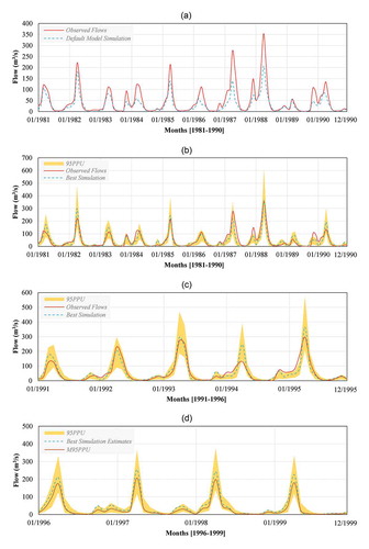
At the first step of the calibration process, the br² value increases to 0.51 (b = 0.58) by fitting and then fixing TLAPS and PLAPS parameters. At the next step, the adjustment of 6 snow-related parameters detected as sensitive according to the conducted one-at-a-time sensitivity analyses to their best-performing values raises the br² value to 0.60 (b = 0.74). Although a significant improvement in the simulation of peak flow rates is achieved at the end of the first two steps of the calibration process, the overall model performance is still not sufficient. At the last step of the model calibration, a total of 14 sensitive modelling parameters in the groundwater, soil, hydrologic response unit, management and main channel input files are adjusted by repeating combined iterations three times. Figure 5(b) shows the monthly simulated and observed streamflow values at the Besiri station location. Accordingly, it is seen that the model simulates the streamflow well. The list of parameters included in the calibration process is presented with their calibrated ranges and best-performing values in Table 3.

Table 3. List of calibrated parameters.

Sensitive parameter^a	Calibratedparameter range	Best-performing parameter value
Step 1: Calibration of precipitation and temperature lapse rates and fixing them to their best simulation values
Temperature lapse rate (°C/km), v__TLAPS.sub^b Precipitation lapse rate (mm H2O/km), v__PLAPS.sub	−7.345^c 9.98
Step 2: Calibration of sensitive snow-related parameters and fixing them to their best simulation values
Melt factor for snow on June 21 (mm H2O/°C-day), v__SMFMX.bsn Snowfall temperature (°C), v__SFTMP.bsn Snow pack temperature lag factor, v__TIMP.bsn Melt factor for snow on December 21 (mm H2O/°C-day), v__SMFMN.bsn Snow melt base temperature (°C), v__SMTMP.bsn Minimum snow water content that corresponds to 100% snow cover (mm H2O), v__SNOCOVMX.bsn	11.499 5.892 0.251 3.706 −8.767 158.578
Step 3: Calibration of other sensitive modelling parameters
Available water capacity of the soil layer (mm H2O/mm soil), r__SOL_AWC().sol Depth from soil surface to bottom of layer (mm), r__SOL_Z().sol Baseflow alpha factor (1/days), v__ALPHA_BF.gw Initial SCS runoff curve number for moisture condition II, r__CN2.mgt Saturated hydraulic conductivity (mm/hr), r__SOL_K().sol Moist bulk density (mg/m^3 or g/cm^3), r__SOL_BD().sol Plant uptake compensation factor, v__EPCO.hru Effective hydraulic conductivity in main channel alluvium (mm/hr), v__CH_K2.rte Average slope steepness (m/m), r__HRU_SLP.hru Groundwater delay time (days), v__GW_DELAY.gw Deep aquifer percolation fraction, v__RCHRG_DP.gw Soil evaporation compensation factor, v__ESCO.hru Threshold depth of water in the shallow aquifer required for return flow to occur (mm H2O), v__GWQMN.gw Groundwater revap coefficient, v__GW_REVAP.gw	[−0.99, 2] [−0.7, 1.9] [0.2, 1] [−0.04, 0.1] [−0.99, 249.3] [0.02, 0.56] [0, 0.7] [−0.01, 500] [−0.5, 0.2] [0, 400] [0.4, 1] [0, 0.6] [0, 4000] [0.02, 0.15]	−0.927 0.769 0.858 0.044 239.539 0.422 0.155 443.499 0.055 219.6 0.882 0.074 3092 0.077

^aThe parameters are listed starting from the most sensitive one for each step of the calibration process.

^bThe qualifier (v__) refers to the substitution of a parameter by a value from the given range, while (r__) refers to a relative change in the parameter for which the current value is multiplied by 1 plus a factor in the given range.

^cThe fixed values indicate that a parameter is fitted and then fixed.

The calibrated parameter ranges provide a P factor value of 0.73 and a R factor value of 0.53 and the objective function br², NSE, PBIAS and RSR statistics of the best simulation are 0.71, 0.81, 6.5% and 0.44, respectively. Table 4 includes the simulation statistics obtained throughout the calibration process in detail. According to Moriasi et al. (2007), the calibrated model performance is identified as very good in terms of the obtained NSE, PBIAS and RSR values. Although it is targeted to increase the slope of the linear regression line between the measured and simulated flow rates to a value around 1, the conducted calibration procedure raises the br² value to 0.71 and the b value to 0.87. Nevertheless, obtaining a coefficient of determination of 0.82, on which values greater than 0.6 are considered as acceptable, shows that the calibrated model performance is quite sufficient to simulate monthly flow rates (Santhi et al. 2001, Moriasi et al. 2007). While the 95PPU band covers 73% of the observed data as above 70% suggested by Abbaspour et al. (2015), the obtained R factor below the recommended value of 1 makes model verification necessary to check over conditioning of the model on a single calibration dataset.

Table 4. Simulation statistics for the calibration and validation periods.

Simulation period	Stage	P factor	R factor	br^2	b	NSE	PBIAS(%)	RSR
1981–1990	Default model	-	-	0.49	0.56	0.68	37.2	0.56
1981–1990	Model calibration: Step 1	-	-	0.51	0.58	0.70	35.8	0.55
	Model calibration: Step 2	-	-	0.60	0.74	0.75	28.8	0.50
	Model calibration: Step 3	0.73	0.53	0.71	0.87	0.81	6.5	0.44
1991–1995	Model validation	0.75	0.50	0.86	0.99	0.84	0.3	0.39

The calibrated model validation conducted with the monthly streamflow records of the Besiri station for the 1991–1995 period results with a better agreement between the observed and simulated flows than in the calibration period. Figure 5(c) presents the outcome of the validation period with the statistical performance provided in Table 4. When the P factor and R factor indices of the validation period are evaluated, it is seen that a reasonable P factor can be achieved without the expense of a large R factor and it shows the strength of the model calibration.

When the best simulation estimates for the validation period are analysed to check the usability of the best-performing parameter set of the calibration stage in streamflow predictions, the statistical performance of the best simulation estimates is found to be similar to that of the best simulation, as detailed in Table 5. Moreover, the simulation statistics of the obtained M95PPU values are calculated for both the calibration and validation periods to analyse the prediction performance of the calibrated SWAT model based on the M95PPU values. Accordingly, while the model performance in terms of M95PPU is identified to be sufficient for all quantitative statistics in the calibration and validation periods, the calculated PBIAS values are too high compared to those of the best simulation and best simulation estimates (Table 5).

Table 5. Comparison of the simulation statistics for the calibration and validation periods.

Model prediction	br^2	b	NSE	PBIAS(%)	RSR	Mean_sim(Mean_obs)	StdDev_sim(StdDev_obs)
Calibration period (1981–1990)
Best simulation	0.71	0.87	0.81	6.5	0.44	43.78 (46.84)	58.90 (61.35)
M95PPU	0.60	0.75	0.75	24.6	0.50	34.37 (46.84)	50.18 (61.35)
Validation period (1991–1995)
Best simulation	0.86	0.99	0.84	0.3	0.39	55.45 (55.60)	75.62 (69.88)
M95PPU	0.74	0.84	0.85	21.4	0.39	43.70 (55.60)	62.99 (69.88)
Best simulation estimates	0.85	0.98	0.84	0.1	0.39	55.43 (55.60)	75.57 (69.88)

3.2 Estimation of monthly irrigation return flow fractions

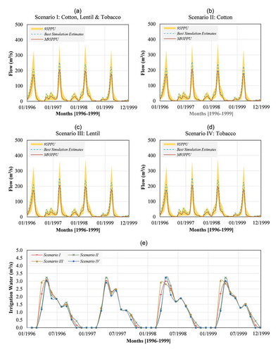
The natural monthly streamflow rates of the Besiri station from 1996 to 1999, that corresponds to the period from the commissioning date of the Kozluk irrigation to the last date of the available station records, are predicted by using the best-performing parameter set of the model calibration stage and the calibrated parameter ranges separately. The best simulation estimates and the 95PPU band of the simulated flows are presented in Fig. 5(d). The mean and standard deviation of the predicted flow rates are, respectively, 42.33 and 62.80 for the best simulation estimates and 32.38 and 50.99 for the M95PPU values. Similarly, the monthly streamflow rates of the Besiri station are simulated through the prediction period to obtain the best simulation estimates and the M95PPU values under the considered cultivation scenarios. Figure 6(a–d) show the time series of the calibrated SWAT model estimates for the 1996–1999 period with the introduction of, respectively, the combined cotton, lentil and tobacco cultivation (Scenario I), cotton only cultivation (Scenario II), lentil only cultivation (Scenario III) and tobacco cultivation only (Scenario IV) scenarios.

Figure 6. Calibrated model estimates for the 1996–1999 period under the effects of each cultivation scenario and the amounts of water supply diverted to the irrigation area in each scenario: (a) Scenario I, (b) Scenario II, (c) Scenario III, (d) Scenario IV and (e) irrigation water amounts.

The performance of the calibrated model after introducing the agricultural activities in the basin is evaluated against the monthly flow records of the Besiri station for the 1996–1999 period in terms of the statistics of br², NSE, PBIAS and RSR. Table 6 includes the simulation statistics of the best simulation estimates and the M95PPU values under each of the considered scenarios. It is observed that the introduced crop pattern does not affect the quantitative simulation statistics and the model performance can be judged as good for both the best simulation estimates and the M95PPU values (Moriasi et al. 2007). However, while the positive PBIAS statistics of the model predictions based on the M95PPU values indicate model underestimation, the negative PBIAS values of the best simulation estimates indicate model overestimation (Gupta et al. 1999).

Table 6. Comparison of the simulation statistics for the prediction period (1996–1999).

Model prediction	br^2	b	NSE	PBIAS (%)	RSR	Mean_sim(Mean_obs)	StdDev_sim(StdDev_obs)
Scenario I: Cotton, lentil & tobacco
M95PPU	0.83	0.96	0.84	13.1	0.40	31.73 (36.53)	50.72 (48.94)
Best simulation estimates	1.00	1.18	0.71	−14.0	0.54	41.64 (36.53)	62.68 (48.94)
Scenario II: Cotton
M95PPU	0.83	0.96	0.84	13.1	0.40	31.74 (36.53)	50.74 (48.94)
Best simulation estimates	1.00	1.18	0.70	−14.0	0.54	41.64 (36.53)	62.79 (48.94)
Scenario III: Lentil
M95PPU	0.83	0.96	0.84	13.1	0.40	31.73 (36.53)	50.71 (48.94)
Best simulation estimates	1.00	1.18	0.71	−13.9	0.54	41.62 (36.53)	62.57 (48.94)
Scenario IV: Tobacco
M95PPU	0.83	0.96	0.84	13.1	0.40	31.74 (36.53)	50.64 (48.94)
Best simulation estimates	1.00	1.18	0.70	−14.2	0.54	41.72 (36.53)	62.80 (48.94)

The amounts of water supply diverted to the irrigation area in the cultivation scenarios are close to each other, as presented in Fig. 6(e). However, while the irrigation requirements of cotton, lentil and tobacco are 848.5, 881.8 and 763.2 mm/year in scenarios II, III and IV, respectively, these requirements are determined in turn as 641.6, 1000.3 and 912.9 mm/year for Scenario I. In addition, the irrigation requirement of the whole irrigated area in Scenario I is 861.2 mm/year. Although the determined irrigation requirements of the analysed crops are not very different to the values reported in Ilhan and Utku (2000), the differences between the water requirements of these crops in the uniform cultivation scenarios and those in the combined cultivation scenario demonstrate the importance of the knowledge about the spatial distribution of crop pattern.

The model predictions of the 1996–1999 period obtained with and without the introduction of upstream agricultural activities are compared on a monthly basis for the best simulation estimates and M95PPU values separately. Figure 7(a–d) demonstrate these comparisons conducted under scenarios I, II, III and IV, respectively. The monthly rates of return are calculated as the percentages of the ratios of the monthly irrigation return amounts to the corresponding monthly amounts of water supply diverted to the irritation area, as listed in Table 7. When the obtained monthly river-return ratios for the considered cultivation scenarios are analysed, it is seen that the return ratios range between 17.9 and 67.8%, vary month to month, differ from one crop type to another and change depending on the use of the best simulation estimates and M95PPU values. In addition, when the return ratios are evaluated on an annual basis for each of the cultivation scenarios, it is observed that the annual return ratios range between 33.8 and 42.3% for the use of the M95PPU values and between 35.5 and 36.1% for the use of the best simulation estimates (Table 7). The resultant monthly and annual irrigation return flow ratios are quite different from the rate of 20% used as an assumption for the Kozluk irrigation scheme in the planning reports of the upper Tigris Basin projects (Ilisu Hydropower Consultants 1983, Ilisu Environment Group 2005, Enersu 2008). In the existing literature, there are not any researches investigating irrigation return flow quantities from cotton, tobacco and lentil fields in such a semi-arid agricultural region as the Garzan Basin, which makes it difficult to judge the reliability of the obtained results.

Table 7. Monthly and annual irrigation return flow ratios using M95PPU and best simulation estimates values.

	Irrigation return flow ratio (%)
	Scenario I		Scenario II		Scenario III		Scenario IV
Months	M95PPU	Best simulation estimates	M95PPU	Best simulation estimates	M95PPU	Best simulation estimates	M95PPU	Best simulation estimates
1	0.00	0.00	0.00	0.00	0.00	0.00	0.00	0.00
2	0.00	0.00	0.00	0.00	0.00	0.00	0.00	0.00
3	0.00	0.00	0.00	0.00	0.00	0.00	0.00	0.00
4	17.93	31.44	-^a	25.75	35.57	30.31	-^a	27.56
5	63.98	33.27	63.20	33.31	67.75	33.33	50.05	33.86
6	56.22	32.75	66.07	33.31	50.75	32.71	57.33	32.86
7	39.06	37.70	40.09	37.57	38.15	37.81	41.70	37.59
8	38.67	43.34	38.83	43.18	38.55	43.47	40.61	43.32
9	46.66	39.24	47.23	38.90	45.98	39.43	53.44	39.52
10	34.39	34.97	31.68	33.95	32.29	36.39	51.02	34.64
11	29.96	43.32	47.82	37.77	0.00	0.00	0.00	0.00
12	0.00	0.00	0.00	0.00	0.00	0.00	0.00	0.00
Annual	40.71	35.92	40.36	35.48	42.23	35.79	33.77	36.08

^aIrrigation return flow ratio cannot be determined because the difference between the monthly mean M95PPU values obtained with and without introducing the upstream irrigation activities is higher than the monthly mean flow rate diverted to the irrigation area.

Figure 7. Comparisons of the monthly means of the model predictions obtained with and without introducing the upstream agricultural activities: (a) Scenario I, (b) Scenario II, (c) Scenario III and (d) Scenario IV.

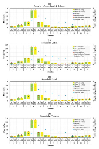
Although the statistical streamflow prediction performances in all the analysed periods are sufficient to say that the model does not require a further calibration, the differences in the streamflow estimates and, hence, the range of the obtained irrigation return ratios is quite large for some months, especially with high flow rates. The effects of crop pattern change on the monthly and annual ranges of return rates are relatively small due to the close amounts of irrigation requirement in the considered cultivation scenarios. However, the calculated return rates can significantly differ depending on the use of the best simulation estimates and M95PPU values. This is especially the case for the months of April, May and June, as can be seen in Table 7. Due to the prediction sensitivity of the proposed method, the return ratios in April for Scenario II and IV cannot be calculated using the M95PPU values because of the higher net water usages than the amounts of water supply diverted to the irrigation area. For the months of May and June, the return rates calculated with the M95PPU values are too high to be realistic in all cultivation scenarios. Although there are some studies in the literature reporting the irrigation return ratios above 50% for their cases, such high rates were obtained mostly for paddy fields (Jalota and Arora 2002, Dewandel et al. 2008, Jimenez-Martinez et al. 2009). These findings demonstrate the weakness of the calibrated SWAT model in simulating discharge peaks, especially in terms of the M95PPU values, probably due to the poor characterisation of snow-related processes and groundwater-river interact in this partly mountainous watershed (Rostamian et al. 2008).

As there are limited data available for the region of study, it cannot be possible to overcome this weakness. Even the limits of the absolute parameter ranges of SWAT are utilized for some of the sensitive modelling parameters in the calibration process, as in the cases of the studies of Rostamian et al. (2008), Zhang et al. (2014) and Dhami et al. (2018). However, no further improvement is obtained in decreasing the month-based prediction uncertainty ranges. Nevertheless, the obtained ranges of return rates on monthly and annual bases give an idea about the correctness of the rule-of-thumb value assumed for the Kozluk irrigation scheme. In general, the return ratios are evaluated to be in the range 20–40% and this range is consistent with the calculated return rates using the best simulation estimates (Oosterveld et al. 1978, Keys 1981). Therefore, for the Kozluk irrigation, it can be advised to use the return rates based on the best simulation estimates, rather than the ones calculated with the M95PPU values. There is no doubt that more realistic results can be obtained by the proposed method if regional fine-scale datasets are used in model construction.

4 Summary and conclusions

This study presents the steps carried out to assess the return flow ratio of an irrigation abstraction when the only data in hand is the flow records of a downstream stream-gauging station, with the example of the Kozluk irrigation scheme. This evaluation is based on the streamflow predictions of the SWAT model constructed with the coarse-scale DEM, LULC and soil data from open source databases and the daily weather records of the nearby meteorological stations. After calibrating and validating the monthly flow simulations of the generated SWAT model against the monthly streamflow records of the Besiri station located at just downstream of the irrigated area for the period prior to the initiation of the irrigations in the Kozluk region, the flow rates at the Besiri station location are simulated with and without introducing the considered cultivation scenarios for the prediction period from the commissioning year of the irrigation plan to the last date of the available flow records. Accordingly, by comparing the natural streamflow estimates and their corresponding values under the influence of each cultivation scenario, the admissible ranges of irrigation return rate are determined on monthly and annual bases. The results indicate that the rule-of-thumb value used for the Kozluk scheme in the planning reports of the upper Tigris Basin projects is quite out of these ranges.

Although the use of coarse-scale data in the SWAT model development does not lead to unsatisfactory simulation performances in terms of the considered statistical evaluation indexes, the changes of the obtained rate of returns depending on the use of the best simulation estimates and M95PPU values demonstrate the effect of the model predictions on the resultant return ratios. Moreover, the dependence of the obtained rate of returns to the crop pattern changes makes irrigation project-based analyses necessary. Therefore, instead of using river-return assumptions in water potential analyses, the effects of each upstream irrigation activity on flow regimes should be assessed separately using fine-scale datasets as much as possible in model development to more accurately utilize the irrigation and hydropower potentials of the upper Tigris Basin projects and the others under the same conditions.

Acknowledgements

This work was supported by the Kirsehir Ahi Evran University Scientific Research Projects Coordination Unit under grant number MMF.A4.17.005.

Disclosure statement

No potential conflict of interest was reported by the author.

Additional information

Funding

This work was supported by the Kirsehir Ahi Evran University Scientific Research Projects Coordination Unit [MMF.A4.17.005].

References

- Abbaspour, K.C., 2015. SWAT-CUP2: SWAT calibration and uncertainty programs - a user manual. Duebendorf, Switzerland: Eawag - Swiss Federal Institute of Aquatic Science and Technology.
- Abbaspour, K.C., Johnson, C.A., and van Genuchten, M.T., 2004. Estimating uncertain flow and transport parameters using a sequential uncertainty fitting procedure. Vadouse Zone Journal, 3 (4), 1340–1352. doi:10.2136/vzj2004.1340
- Abbaspour, K.C., et al., 2015. A continental-scale hydrology and water quality model for Europe: calibration and uncertainty of a high-resolution large-scale SWAT model. Journal of Hydrology, 524, 733–752. doi:10.1016/j.jhydrol.2015.03.027
- Abbaspour, K.C., et al., 2007. Modelling hydrology and water quality in the pre-alpine/alpine Thur watershed using SWAT. Journal of Hydrology, 333 (2–4), 413–430. doi:10.1016/j.jhydrol.2006.09.014
- Arnold, J.G., et al., 2013. SWAT 2012 input/output documentation. Texas: Texas Water Resources Institute.
- Boisrame, G., 2011. WGNmaker4.1.xlsm Microsoft Excel macro [online]. Available from: https://swat.tamu.edu/software/links/ Accessed 25 December 2017.
- Chen, S.-K. and Liu, C.W., 2002. Analysis of water movement in paddy rice fields (I) experimental studies. Journal of Hydrology, 260 (1–4), 206–215. doi:10.1016/S0022-1694(01)00615-1
- Chen, S.-K., Liu, C.W., and Huang, H.-C., 2002. Analysis of water movement in paddy rice fields (II) simulation studies. Journal of Hydrology, 268 (1–4), 259–271. doi:10.1016/S0022-1694(02)00180-4
- Dewandel, B., et al., 2008. An efficient methodology for estimating irrigation return flow coefficients of irrigated crops at watershed and seasonal scale. Hydrological Processes, 22 (11), 1700–1712. doi:10.1002/(ISSN)1099-1085
- Dhami, B., et al., 2018. Evaluation of the SWAT model for water balance study of a mountainous snowfed river basin of Nepal. Environmental Earth Sciences, 77 (21). doi:10.1007/s12665-017-7210-8
- DSI (General Directorate of State Hydraulic Works), 2007. Akım gözlem istasyonları, aylık toplam akımlar (1954–2000) [Flow gauging stations, monthly total flows (1954–2000)]. Ankara: General Directorate of State Hydraulic Works.
- EIE (General Directorate of Electrical Power Resources Survey and Development Administration), 2003. Aylık ortalama akımlar (1935–2000) [Monthly mean discharges (1935–2000)]. Ankara: General Directorate of Electrical Power Resources Survey and Development Administration.
- Enersu (Enersu Engineering Consultancy Construction Industry and Trade Limited Company), 2008. Garzan Barajı ve HES revize fizibilite raporu [Garzan Dam and HEPP revised feasibility report]. Ankara: Enersu Engineering Consultancy Construction Industry and Trade Limited Company.
- EU-JRC (European Commission - Joint Research Centre), 2006. The global land cover 2000 (GLC2000) products [online]. Available from: http://forobs.jrc.ec.europa.eu/products/glc2000/products.php Accessed 20 December 2017.
- FAO (Food and Agriculture Organization of the United Nations), 2007. Digital Soil Map of the World (DSMW) [online]. Available from: http://www.fao.org/geonetwork/srv/en/metadata.show?id=14116 Accessed 20 December 2017.
- Faramarzi, M., et al., 2013. Modeling impacts of climate change on freshwater availability in Africa. Journal of Hydrology, 480, 85–101. doi:10.1016/j.jhydrol.2012.12.016
- Glavan, M. and Pintar, M., 2012. Strengths, weaknesses, opportunities and threats of catchment modelling with Soil and Water Assessment Tool (SWAT) model. In: P. Nayak, ed. Water resources management and modeling. Rijeka: InTech, 39–64.
- Gosain, A.K., et al., 2005. Return-flow assessment for irrigation command in the Palleru river basin using SWAT model. Hydrological Processes, 19 (3), 673–682. doi:10.1002/(ISSN)1099-1085
- Gupta, H.V., Sorooshian, S., and Yapo, P.O., 1999. Status of automatic calibration for hydrologic models: comparison with multilevel expert calibration. Journal of Hydrologic Engineering, 4 (2), 135–143. doi:10.1061/(ASCE)1084-0699(1999)4:2(135)
- Ilhan, A.I. and Utku, M., 2000. GAP sulama alanında bitki su tüketimi ve bitki su gereksinimi [Plant water consumption and requirement of the GAP irrigation area]. Ankara: General Directorate of State Meteorological Works.
- Ilisu Environment Group, 2005. Ilisu Dam and HEPP environment impact assessment report with enclosures. Ankara: Ilisu Environment Group: Hydro Concepts Engineering, Hydro Quebec International and Archeotec Incorporated.
- Ilisu Hydropower Consultants, 1983. The Cizre Dam and HEPP project feasibility report. Ankara: Ilisu Hydropower Consultants: Binnie & Partners, Gizbili Consultancy Engineering, James Williamson & Partners, Kennedy & Donkin and COBA.
- Jafari, H., et al., 2012. Time series analysis of irrigation return flow in a semi-arid agricultural region, Iran. Archives of Agronomy and Soil Science, 58 (6), 673–689. doi:10.1080/03650340.2010.535204
- Jalota, S.K. and Arora, V.K., 2002. Model-based assessment of water balance components under different cropping systems in north-west India. Agricultural Water Management, 57 (1), 75–87. doi:10.1016/S0378-3774(02)00049-5
- Jimenez-Martinez, J., et al., 2009. A root zone modelling approach to estimating groundwater recharge from irrigated areas. Journal of Hydrology, 367 (1–2), 138–149. doi:10.1016/j.jhydrol.2009.01.002
- Keys, J.W., 1981. Grand Valley irrigation return flow case study. Journal of the Irrigation and Drainage Division (ASCE), 107, 221–232.
- Lemann, T., Roth, V., and Zeleke, G., 2017. Impact of precipitation and temperature changes on hydrological responses of small-scale catchments in the Ethiopian Highlands. Hydrological Sciences Journal, 62 (2), 270–282. doi:10.1080/02626667.2016.1217415
- Liersch, S., 2003. Dewpoint estimation programs: dew.exe and dew02.exe [online]. Available from: https://swat.tamu.edu/software/links/ Accessed 25 December 2017.
- MGM (Turkish State Meteorological Service), 2018a. Daily precipitation, maximum and minimum air temperature, relative humidity and wind speed records of the Batman, Mus and Siirt meteorological stations (1979–1999). Ankara: Turkish State Meteorological Service.
- MGM (Turkish State Meteorological Service), 2018b. Long-term all parameters bulletins for the Batman, Mus and Siirt meteorological stations. Ankara: Turkish State Meteorological Service.
- MGM (Turkish State Meteorological Service), 2018c. Annual maximum precipitation records in standard times for the Batman, Mus and Siirt meteorological stations. Ankara: Turkish State Meteorological Service.
- Mohan, S. and Vijayalakshmi, D.P., 2009. Prediction of irrigation return flows through a hierarchical modeling approach. Agricultural Water Management, 96 (2), 233–246. doi:10.1016/j.agwat.2008.07.013
- Moriasi, D.N., et al., 2007. Model evaluation guidelines for systematic quantification of accuracy in watershed simulations. Transactions of the ASABE, 50 (3), 885–900. doi:10.13031/2013.23153
- Neitsch, S.L., et al., 2011. Soil and water assessment tool theoretical documentation version 2009. Texas: Texas Water Resources Institute.
- Oosterveld, M., McMullin, R.W., and Toogood, J.A., 1978. Return flow and soil salts in two drainage basins. Journal of the Irrigation and Drainage Division (ASCE), 104 (4), 361–371.
- Ozcan, Z., Kentel, E., and Alp, E., 2016. Determination of unit nutrient loads for different land uses in wet periods through modelling and optimization for a semi-arid region. Journal of Hydrology, 540, 40–49. doi:10.1016/j.jhydrol.2016.05.074
- Rostamian, R., et al., 2008. Application of a SWAT model for estimating runoff and sediment in two mountainous basins in central Iran. Hydrological Sciences Journal, 53 (5), 977–988. doi:10.1623/hysj.53.5.977
- Santhi, C., et al., 2001. Validation of the SWAT model on a large river basin with point and nonpoint sources. Journal of the American Water Resources Association, 37 (5), 1169–1188. doi:10.1111/j.1752-1688.2001.tb03630.x
- Schuol, J., et al., 2008. Estimation of freshwater availability in the West African sub-continent using the SWAT hydrologic model. Journal of Hydrology, 352 (1–2), 30–49. doi:10.1016/j.jhydrol.2007.12.025
- Singh, K.B., Gajri, P.R., and Arora, V.K., 2001. Modelling the effects of soil and water management practices on the water balance and performance of rice. Agricultural Water Management, 49 (2), 77–95. doi:10.1016/S0378-3774(00)00144-X
- Suis and Sial (Suis Project Engineering and Consultancy Limited Company & Sial Geosciences Survey and Consultancy Limited Company Joint Venture), 2001. GAP, Batman-Silvan Projesi planlama raporu [GAP, the Batman-Silvan Project planning report]. Ankara: Suis Project Engineering and Consultancy Limited Company & Sial Geosciences Survey and Consultancy Limited Company Joint Venture.
- SWAT-PHU, 2017. Potential Head Unit (PHU) program [online]. Available from: https://swat.tamu.edu/software/potential-heat-unit-program/ Accessed 25 December 2017.
- USGS (United States Geological Survey), 2014. Shuttle Radar Topography Mission (SRTM): 1 arc-second global elevation database [online]. Available from: https://earthexplorer.usgs.gov/ Accessed 20 December 2017.
- Yalcin, E. and Tigrek, S., 2019. The Tigris hydropower system operations: the need for an integrated approach. International Journal of Water Resources Development, 35 (1), 110–125. doi:10.1080/07900627.2017.1369867
- Zhang, X., Xu, Y.-P., and Fu, G., 2014. Uncertainties in SWAT extreme flow simulation under climate change. Journal of Hydrology, 515, 205–222. doi:10.1016/j.jhydrol.2014.04.064