Anomalies in the US precipitation extremes and their association with different modes of climate variability

ABSTRACT

In this study, we investigate the temporal oscillations of precipitation extremes in different climate regions of the United States. We apply quantile perturbation analysis to average daily precipitation and, to 1041 weather stations with high-quality data from 1900 to 2016. Moreover, we explore the relationship between the extreme precipitation and different well-known cyclical climate modes. Overall, the analysis of average daily precipitation identifies a drier condition in the middle decades of the twentieth century and, a wetter climate in the early century and recent decades. Moreover, the in situ analysis reveals a significant anomaly, mainly prevalent in the Central and Southern regions of the United States. We applied a finite set of linear regression models with different combinations of cyclical climate modes to inform the variability of anomalies with best performing models. Our results highlight the dominant effect of ENSO and NAO in the wide area of the United States.

KEYWORDS:

• extreme precipitation
• quantile perturbation analysis
• anomalies
• cyclical climate variability

Editor A. CastellarinAssociate editor J. Rodrigo-Comino

Introduction

Climate is changing and many parts of the world face a shift toward wetter conditions. The fifth report of the Intergovernmental Panel on Climate Change (IPCC (Intergovernmental Panel on Climate Change) 2013) substantiates this alteration through the change of rainfall statistics and the increase in the median of annual maximum daily precipitation. Although, the extreme precipitations are increasing at global scale (Lehmann et al. 2015) over different regions their trends substantially deviate (Donat et al. 2013). Given their profound societal/economic impacts, understanding the variability of extremes is of primary importance in decision-making and hydrosystem planning (Abdi and Yasi 2015, Mazrooei et al. 2015, Najafi et al. 2018, 2018, 2019, Pournasiri Poshtiri et al. 2018, Mcphillips et al. 2018, Armal and And Al-Suhili 2019). In recent years, several studies focused on the analysis of trends and variability in precipitation extremes at the global (Westra et al. 2013, Alexander et al. 2006, Asadieh and Krakauer 2015; Fischer and Knutti 2014); national (Karl and Knight 1998, Groisman et al. 2004, Balling and Goodrich 2011, Zhu 2013, Sun and Lall 2015); and regional scales (Villarini et al. 2011, Shephard et al. 2014, Parr et al. 2015, Manzano-Agugliaro et al. 2015, Nandargi et al. 2016, García et al. 2018). At the global scale (Westra et al. 2013) show that the trend in extreme precipitation over the majority of land-based observing stations is increasing. Asadieh and co-author (Asadieh and Krakauer 2015) conclude the same findings, using both climate models and observation data. Different emissions scenarios indicate a rise in the simulated extreme precipitation over tropical and extratropical regions (O’Gorman and Schneider 2009, Kharin et al. 2013), while over subtropical, this rate grows faster than the mean (IPCC (Intergovernmental Panel on Climate Change) 2013).

Analysis of precipitation in the USA shows important differences in trends of different climate regions. From the second half of the twentieth century, significant increasing trends are observed in north-central and eastern regions of the country and non-significant shift in parts of West and Southern regions (Knutson et al. 2014). Most parts of the country have increased in both intensity and frequency of extremes, yet Northeast demonstrates the largest uptrend (Easterling et al. 2017). Similar studies verify an upward trend in the intensity of extreme precipitation over Northeast (Spierre and Wake 2010, Krakauer 2014) and Midwest (Villarini et al. 2011). In the analysis of extreme frequency across the USA, Armal et al. (2018) identified the Northeast, Central and Midwest regions (Northern Rockies and Plains, Upper Midwest, Ohio Valley) with an overall statistically significant monotonic trend.

In addition to secular trend signals, statistically significant trends might be due to the cyclicity of the hydroclimatic systems (NRC (National Research Council) 1999; Cohn and Lins 2005). The quasi-periodic nature of climate often translates into periods of increasing or decreasing extreme events depending on the climate phase (Armal et al. 2018). Researchers apply large-scale ocean–atmosphere conditions to understand the local-scale manifestations of this climate cyclicity in different regions. The well-known examples, frequently studied in US climate are El Niño Southern Oscillation (ENSO), Pacific Decadal Oscillation (PDO), North Atlantic Oscillation (NAO) and Atlantic multi-decadal oscillations (AMO).

The ENSO is associated with the increase in extreme frequency along the east coast and equatorward shift in the storm track in the North Pacific (Eichler and Higgins 2006). Additionally, the analyses of global coupled climate model characterize the El Niño seasons with increases in intense precipitation in the Southwest USA and systematic shift in this pattern toward the east (Meehl et al. 2007). Similar studies documented the La Niña impact, particularly during winter time, on the anomaly of precipitation along the Pacific coast of the USA (Castello and Shelton 2004), the Southwest and Florida (Gershunov and Cayan 2003). Further, NAO variability influences the winter precipitation in the eastern United States and, leads to significant increases in the occurrence of snow in the Northeast (Durkee et al. 2008). Other studies linked NAO to precipitation variability of the Midwest and Southwest (Andresen et al. 2012, L’Heureux et al. 2014). Although Archambault et al. (2008) argue that the NAO influence is only significant in combination with other climate drivers, recent studies highlight its impact on US extreme rainfall (Whan and Zwiers 2017).

Moreover, PDO fluctuations associate to the increases in the occurrence of wet days and heavy precipitation days over the western/southern United States (Higgins et al. 2007). Studies link the synergized impact of PDO and ENSO to the climate and precipitation variability in the western United States (Goodrich 2007, Pavia et al. 2016). The fact that the long-term effect of PDO can extend up to three decades (Mantua and And Hare 2002) emphasizes its importance over longer windows.

The AMO is another climate driver frequently studied in the climate variability of the USA. The importance of AMO lies in its widespread influence and multilectal oscillation (Kerr 2000). Researchers connect the impact of the warming phase of AMO to decreases in annual rainfall totals over the USA (Enfield et al. 2001). The AMO also associated with the increase of rainfall intensity in the central USA (Curtis 2008), and duration in south Florida (Teegavarapu et al. 2013).

To understand trends and variability of precipitation extremes, studies often apply a trend analysis or a type of fitting regression on a limited time-series data of block maxima or peak over a threshold (Armal et al. 2018). These analyses mainly account for variability in above-threshold values (positive anomalies or wetter than normal) and systematically disregard the variability of negative anomalies (drier than normal). In this study, we apply the quantile perpetuation method (QPM) to investigate the anomaly of extreme precipitation in different regions of the USA. The robustness of the QPM to amalgamate aspects of frequency is an asset in extreme value analysis (Nyeko-Ogiramoi et al. 2013) and to detect both positive/negative anomalies of time series. Various researchers have applied the QPM on meteorological and hydrological variables over different regions and correlated these anomalies with the variation in the large-scale climate modes (Taye and Willems 2012, Willems 2013, Onyutha and Willems 2017). Here, we apply the QPM to investigate the variability of extreme precipitation, using high-quality and long-term observation data in the USA. Further, we investigate the linkages of the extreme variability in different climate regions to the large-scale ocean–atmosphere interactions.

Data and methods

Precipitation

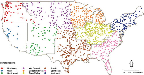
Initially, the total daily precipitation for 12 244 stations across the USA extracted from the Global Historical Climatology Network (GHCN) daily database¹ We selected all the stations that have at least 90 years of data over 1900–2016 (117 years). Here, we consider a year with data only if the percentage of non-available data in that year is below 20%. Figure 1 presents the location of 1041 stations across the country, as the results of the cleaning process. The map also shows the boundary of different climate regions adopted from a temperature-based climate analysis (Karl and Koss 1984). We use these regions to summarize and examine the outcome of this investigation.

Figure 1. Location of the selected stations used in the study in the nine climate regions over the contiguous United States. Adopted from https://www.ncdc.noaa.gov/monitoring-references/maps/us-climate-regions.php. Note that WN Central stands for Western North Central (or Northern Rockies and Plains).

Indices of climate variability

The climate indices applied in this study are the Nino-3.4 ENSO index (obtained from the KNMI Climate Explorer²), PDO³ and NAO⁴ Additionally, the AMO index applied in this study is calculated based on the HADSST dataset of monthly sea-surface temperature (Van Oldenborgh et al. 2009).

In this investigation, we initially explored the temporal oscillations in the average of daily precipitation in different climate regions across the USA. Next, we performed this analysis on data from GHCN meteorological stations and applying the confidence interval obtained from average precipitation perturbation factors, identified the significant anomalies. Finally, we perform a set of regression models to attribute the anomalies of extremes to different modes of climate variability indices.

Computation of precipitation variability

The QPM uses the original fully available data as a baseline period. A continuous and overlapping sliding block of data moves by one time unit of the series (here 1 year of daily precipitation data) to extract several consecutive sub-series. This method considers a time-series of values exceeding a given empirical probabilities and finds the perturbation aspect which determines the relative magnitudes of each sub-series quantiles based on the baseline period. In calculation of perturbation factor, we considered the following steps:

Step 1. Different block sizes (5, 10, 15 years) are selected to extract sub-series from daily average precipitation.

Step 2. The exceedance probability is computed for the values above threshold in each sub-series. In this study, we look at 99% value of the daily non-zero precipitation as a threshold to identify the extremes.

Step 3. Based on the values in the baseline with the same return period, the relative change of extreme in each sub-series block is obtained.

Step 4. Perturbation factor for each block is the average of all relative changes (or anomalies above the stipulated exceedance probability).

Statistical significance of precipitation anomaly

The nonparametric bootstrapping technique is used to derive the confidence interval and evaluate the statistical significance at the 5% level of significance (i.e. the probability of incorrectly rejecting the null hypothesis that the variability is due to natural randomness). For the calculation of the confidence intervals, the values in the full-time series are resampled 5000 time, yielding 5000 different temporal sequence of original data. Applying QPM to each sequence, the anomaly calculations are repeated 5000 times and led to 5000 anomaly values. After ranking these anomaly values, the 2.5 and 97.5 percentile values define the 95% confidence intervals for each block. If the anomaly from original time-series falls outside the confidence interval, is statically significant.

We initially applied a sliding 5-year block period (the name suggested by Tabari et al. 2014, to refer to stipulated moving blocks) to derive temporal oscillation of average daily precipitation and identify the decadal evolution of significant anomaly in each region. Moreover, we expand this analysis by enlarging block window size to evaluate the occurrence of negative/positive anomaly in 10- and 15-year block periods.

Attribution of anomalies to cyclical climate variability

First, applying QPM we computed anomaly of four climate predictors with different quasi-periodic cycles ranging from interannual to decadal to multi-decadal scales (ENSO, NAO, PDO and AMO). Next, we studied the relationship between the anomalies in the extreme precipitation to the anomalies of cyclical climate variability. To quantify the response of variability we use multiple linear regression equation (MLRE) and consider regression coefficients at 5% significance. For each station, we look at 15 regression models, resulting from different combinations of four climate indices, with one to four variables. Here, using different subsets of climate predictors is similar to stepwise regression model with backward/forward selection of predictors to find the best performing model (Onyutha and Willems 2017, Najibi and Devineni 2018). Among different metrics, we use the values of adjusted R² (Ezekiel 1943) to identify the best model among the finite set of models. The selected model informs the values of coefficient regression for incorporated climate predictors.

Results and discussion

Precipitation variability in different climate regions

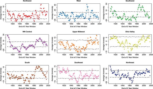
Figure 2 shows the quantile perturbations of extremes in average daily precipitation of nine climate regions. The dots indicate the anomaly in the 5-year stipulated sub-series (the Supplementary material includes the outcome of 10- and 15-year window anomalies), overlaid by a decadal LOWESS (locally weighted scatterplot smoothing) smoothing line. The dashed lines envelop the confidence level calculated from each block. Among different climate regions. The West shows the largest spread of perturbation, ranging from – 20% in the 1950s to +40% in the 1980s. The Southwest indicates a similar pattern, with a strong positive anomaly in the early years of precipitation data, the 1980s and 1990s. Comparable to the Southwest, the Northeast, Southeast and WN Central regions reveal a significant wet period in the early twentieth century. Further, there is a strong negative anomaly around the 1960s, identified in eastern regions including Northeast, Ohio Valley and Upper Midwest. The 1960s dry period has been frequently addressed in climatological aspects of studying drought over these regions (Klugman 1978, Rogers 1993, Seager et al. 2012).

Figure 2. Quantile perturbation analysis on extreme precipitation, using 5-year moving block window size in different climate regions of the USA. The black-dashed lines represent the 95% confidence intervals to define statistically significant perturbations.

Additionally, Table 1 indicates the occurrence of the significant positive/negative anomalies in each decade, reported as a percentage of the total number of 5-year sub-periods. The red and blue labels highlight the maximum positive/negative values for each climate region.

Table 1. Occurrence of the significant positive/negative anomalies in each decade, reported as a percentage of the total number of 5-year sub-periods; the blue and red labels represent the maximum negative and positive percentage for each climate region, respectively.

Climate region

In the majority of regions, a higher rate of positive anomalies in extreme precipitations emerges in recent decades. Whereas, in Ohio Valley, the Southeast and the Northeast, the strongest positive anomaly is observed in the earlier decades of twentieth century. Among different regions, the Northeast shows the highest positive/negative anomaly percentage in the 1900s and 1950s, respectively. Studies suggest that the mean of recent precipitation in parts of the Northeast is 25% above this value before 1970, with even larger increases in the intensity of wet extremes (Krakauer 2014). However, the results of perturbation analysis with the 5-year moving window suggest an oscillatory effect in extreme precipitation in this region, leading to a strong negative anomaly around the 1960s and proceeding to a significant positive anomaly in recent decades (38% in 2000). The analysis of the Northeast climatology associate this oscillation with a variability of the NAO (Seager et al. 2012). Another remarkable feature of the analysis is observed in mid-century decades (the 1930s, 1940s, 1950s, and 1960s), where all the climate regions show a maximum occurrence of the negative anomaly. Here, we witness a sequential pattern that spans from the west to the east of the country. This consistent dry period affects the western part of United States in the 1930s and 1940s (i.e. the West, Southwest and West North Central), moves to central regions (e.g. South) in the 1950s and the eastern region (e.g. Ohio Valley and Northeast) in the 1960s.

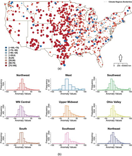
The results of the perturbation analysis unveil the temporal oscillation of anomalies in the average daily precipitation. Next, we apply the 5-year window QPM to understand the variability of the extreme anomaly in the selected meteorological stations. Applying the confidence level obtained from the average daily precipitation, we identify the significant anomaly in each station. Figure 3 shows the spatial distribution of the highest anomaly values and their sign, across different climate regions. The size presents the strength of anomaly and the color scheme indicates the sign of the values. Also, the histograms show the frequency of negative/positive significant anomaly in each region. Clearly, the maximum anomaly is strongly positive through central regions and the southwest of the country (i.e. West North Central, South, and Southwest). Moreover, a positive anomaly is prevalent in the majority of the stations, and few of them show a negative maximum anomaly. The frequency of anomalies in each region indicates that the significant negatives in all the regions are relatively more frequent than significant positives.

Figure 3. (a) Spatial distribution of sign and value of the highest anomaly. (b) The frequency of significant anomalies in different regions. Note that the scale of the y-axis varies for different climate regions.

Attribution of precipitation anomalies to cyclical climate variability

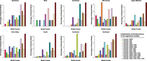
Anomalies of average daily precipitation indicate a drier than an average period, in mid-century of all the regions. However, the majority of the wet periods are observed in the early years and in recent decades of the data. Using attribution analysis, we attempted to understand as to what extent this behavior is related to the cyclicity of different climate influences. Applying the different combination of climate predictors to inform the anomalies will enable us to choose the coefficient regression values from the highest skill model. Here, adjusted R² penalizes the explanatory power of the model for adding more independent variables, and better assess the goodness-of-fit for linear regression analysis (Jeffrey 2018). Figure 4 shows the percentage of stations within each climate region, and which performs better under each combination of climate drivers. Including all the predictors in the majority of regions improves upon the overall range of values, particularly in the Southwest, West North Central and Upper Midwest. However in regions such as the South, single-predictor (here ENSO) models can be more reliable than those with multi-predictors. It is observed through the investigations that different combinations of climate indices yield many models with low goodness of fit. For attribution analysis, we primarily consider the models with adjusted R² higher than 0.25. If none of the models is skillful enough, we discern the corresponding station in our analysis.

Figure 4. The percentage of stations that perform better with different combinations of climate drivers within each climate region.

Figure 5 shows the results of attribution analysis. The boxplots on the top (Fig. 5(a)) present the range of regression coefficient responses values and the maps (Fig. 5(c)) represent their spatial distribution. The bar plots (Fig. 5(b)) compare the significance of different climate influences, applying the ratio of stations with significant response to the total number of stations in each climate region. We consider a climate predictor to be significant if the p value for the null hypothesis that the coefficient is equal to zero (no effect) is less than 0.05.

Figure 5. Coefficient regression values for different climate predictors within each climate region. (a) Boxplots indicating the range of coefficient regressions (variable scale of y-axes). (b). Maps showing the spatial distribution of coefficient of regression values for different climate variables. (c) Barcharts of the significance ratio (ratio of stations with significant response at 5% to the total number of stations) of the climatic variables within each climate region.

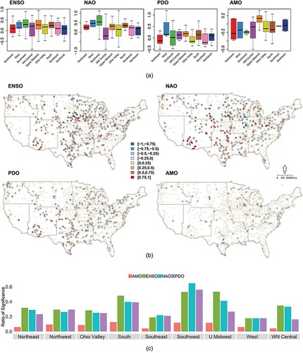
Based on the results, ENSO has a significant positive relationship in the South climate region, the Southwest and the Upper Midwest. These results are consistent with the results found by Gershunov and Cayan (2003), who investigated the associations of ENSO with heavy precipitation events in the USA. In the Southwest, West North Central and Northwest, the significant ratio is relatively high, but the response to ENSO varies substantially. Studies (e.g. Cayan et al. 1999) show that negative SOI values (El Niño) lead to wetter climate over the Southwest, and drier condition in Northwest, while with positive SOI years (La Niña), almost the opposite is observed. Similarly, our anomalies analysis characterizes both regions with high association with ENSO variability. The impact of ENSO on the South and Southeast climate is well documented (Ropelewski and Halpert 1986, Penalba and Rivera 2016, Mourtzinis et al. 2016), mainly in terms of boreal winter and spring precipitation anomaly (Wang and Asefa 2018). However, a few studies (Barsugli et al. 1999, Glantz 2002) explored the potential impact of SOI index variability on the occurrence of summer drought and unusual precipitation on the northern parts of the east coast. The potential impact of other climate and atmospheric drivers complicates our understanding of the impact of ENSO on the Northeast. It is generally observed that, during active years of ENSO, winter precipitation in part of the region has a positive anomaly, while the other part represents a negative anomaly (Mecray 2015). Comparably, the regression models in this analysis show opposing trend values inside the region, but overstate the ENSO impact with a relatively high statistically significant response.

With regard to other climate drivers in the MLRE models, NAO mainly shows a positive connection with many stations across different regions. NAO is the primary mode of atmospheric variability over the Atlantic Ocean and significantly impacts the eastern and northern part of the United States (Durkee et al. 2008). Studies have linked the 1960s Northeast drought to the oscillatory nature of NAO and the seesaw in the pressure and GPH anomalies between the subpolar and subtropical Atlantic Ocean (Seager et al. 2012). In western regions, the impact of NAO in lower elevation area was discussed by Myoung et al. (2015, 2017)), where early warm spring and snow-melting is associated with development of positive NAO. Also, it is shown that during a negative NAO phase, portions of the Midwest, especially eastern sections, experience above-normal precipitation during winter and spring (Andresen et al. 2012). The trend analysis suggests strong positive association of Southwest and significant negative response of West North-Central climate region to NAO variability. The positive NAO is associated with low pressure and wet condition in the Southwest, although it is generally hard to distinguish this relation from the impact of ENSO (L’Heureux et al. 2014). Further, numerous significant stations in the Northeast reveal a moderate positive response to NAO variation.

The other two climate drivers (AMO and PDO) applied in this analysis indicate a relatively lower impact on the anomaly of extreme precipitation. AMO in positive phase links to hurricane activity in the southeast (Curtis 2008), and in phase combination with PDO, it can explain more than half of multi-decadal droughts in the continental United States (Mccabe et al. 2004). However, the 5-year window anomalies analysis cannot manifest the long cyclical oscillation of these climate drivers. The PDO coefficient regression map presents a pattern similar to ENSO, except for the fact that the number of significant responses is notably lower. The PDO impact is significant in the Southwest, Northwest, and South. Moreover, AMO yields a statistically significant but weak and mostly negative association in much of the country, without any dominance in any climate region.

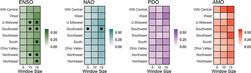
The analysis of 5-year block anomaly indicates the dominant effect of ENSO and NAO in many different climate regions. However, the choice of window size possibly regulates the response of climate regions to different modes of climate variability. Larger window size decreases the range of values but influences the temporal variability of detected anomalies. Hence, we perform the MLRE analysis by 10- and 15-year windows to choose the coefficient response from the model with the highest skill. Figure 6 presents the results of this process. It can be clearly seen from Fig. 6 that the ENSO variability is a consistently dominant effect in the Upper Midwest, Southwest, and Northwest. With the increase in window size, this effect becomes noticeable in the South and Northeast as well. Moreover, NAO shows strong response in the Southwest, with 5- and 15-year window anomaly. In the Upper Midwest, the impact of NAO is more evident for the larger window size. PDO and AMO are not dominant in any of the regions. However, in some regions, such as the West (for PDO), the Upper Midwest and West North Central (for AMO) the response to longer cyclical effects over larger window size becomes stronger.

Figure 6. Coefficient regression values for different climate predictors and different block sizes. The color scheme represents the median of significant coefficient of regression values within each region. Black dots indicate the regions where values are significant in more than 75% of stations. White cells denote that the median coefficient regression is close to zero.

Summary and conclusions

In this study, we explored the space-time variability of extreme precipitation anomaly, across different climate regions of the continental United States. First, we applied 5-year block period QPM to average daily precipitation and investigated the time-oscillation of perturbation factors in each climate region. Using a non-parametric bootstrapping technique we defined the 95% confidence interval to identify the positive/negative significance anomalies. Our results suggest that the occurrence of significant positive anomalies is more frequent in recent periods. However, in the Northeast and Ohio Valley, with their large uptrend and variability, the early decades of the twentieth century present the highest positive anomaly. Moreover, our analysis characterizes the mid-century in all the regions of the USA with significantly drier conditions. We also applied the confidence interval extracted from average daily precipitation to analysis of 1041 high-quality stations across the USA and explored the spatial pattern of the value as well as the sign of the highest anomaly. Our results suggest that negative anomalies are more frequent in all climate regions, but the maximum anomaly is predominately positive for the major part of the country and much stronger toward the south and west.

Furthermore, we investigated the association of extreme anomaly with variability of the large-scale ocean–atmosphere conditions. We informed the anomalies with 15 combinations of four different cyclical climate variability modes and selected the best performing model from the coefficient of regression. Our findings suggest that ENSO and NAO have a more dominant effect in the major part of the country. The ENSO variability greatly influences the Upper Midwest, Southwest and South, the NAO shows a strong response in the Southwest and Upper Midwest, and the PDO shows a similar pattern to ENSO effect but with less significant association. Also, the AMO presents a mainly negative and weak impact on a small number of stations across the country. We also applied the QPM method to understand the time-oscillation of extreme precipitation in different block sizes. Our results show that the impact of ENSO and NAO are more dominant with a 10- and 15-year window anomaly.

The QPM is a simple, yet powerful tool that provides a prompt summary of the variability in different hydrological parameters. Using long historical observation data in the analysis of extremes, enables researchers to attribute the variability in the data to different modes of climate variability, especially ones with lower frequency. However, there are limitations to applying the QPM in the detection of anomalies. The QPM leads to loss of information as a result of the aggregation effect. It may also introduce a false cyclic behavior due to the impact of auto-correlation (Fischer and Schumann 2015). Hence, researchers have employed the non-parametric cumulative rank difference (CRD) method (Onyutha 2016, 2018) or the empirical mode decomposition (EMD) method (Rutkowska et al. 2017) to complement and verify the outcome of the QPM. These methods are robust, but more adapted in the analysis of continuous data. For the case of discrete data such as daily rainfall extremes with an exceedance probability of 1% (and greater), the QPM implementation is more well founded.

Our results provide useful knowledge for various applications that are relying on analysis of extreme precipitation anomalies. However, one can improve the current study by considering the regional characteristics of monitoring stations (e.g. elevation, precipitation characteristics) to gain a deeper insight into the space-time structure of extremes in the United States. Moreover, identifying the effect of lagged dependency can improve attribution analysis and the interaction of climate drivers with precipitation variability.

Acknowledgements

The authors would like to thank The City College of New York, NOAA-CREST program and NOAA Office of Education, Educational Partnership Program. The statements contained within the manuscript/research article are not the opinions of the funding agency or the U.S. government, but reflect the author’s opinions.

Disclosure statement

No potential conflict of interest was reported by the authors.

Supplementary material

Supplemental data for this article can be accessed here.

Additional information

Funding

This study is supported by National Oceanic and Atmospheric Administration Cooperative Science Center for Earth System Sciences and Remote Sensing Technologies (NOAA-CREST) under the Cooperative Agreement [Grant no. NA16SEC4810008]. The statements contained within the article are not the opinions of the funding agency or the U.S. government but reflect the authors’ views.

Notes

¹ https://www.ncdc.noaa.gov/oa/climate/ghcn-daily/..

² http://climexp.knmi.nl.

³ https://www.ncdc.noaa.gov/teleconnections/pdo/.

⁴ https://climatedataguide.ucar.edu/climate-data/hurrell-north-atlantic-oscillation-nao-index-station-based..

References

- Abdi, R. and Yasi, M., 2015. Evaluation of environmental flow requirements using eco-hydrologic–hydraulic methods in perennial rivers. Water Science and Technology. IWA Publishing, 72 (3), 354–363. doi:10.2166/wst.2015.200
- Alexander, L.V., et al., 2006. Global observed changes in daily climate extremes of temperature and precipitation. Journal of Geophysical Research: Atmospheres, 111 (D5). doi:10.1029/2005JD006290
- Andresen, J., et al., 2012. Historical climate and climate trends in the midwestern USA. US National Climate Assessment Midwest Technical Input Report. 1–18.
- Archambault, H.M., et al., 2008. Influence of large- scale flow regimes on cool-season precipitation in the Northeastern United States. Monthly Weather Review, 136 (8), 2945–2963. doi:10.1175/2007MWR2308.1
- Armal, S. and And Al-Suhili, R., 2019. An urban flood inundation model based on cellular automata. International Journal of Water. Inderscience Publishers (IEL), in press, 13, 221. doi:10.1504/IJW.2019.101336
- Armal, S., Devineni, N., and Khanbilvardi, R., 2018. Trends in extreme rainfall frequency in the contiguous united states: attribution to climate change and climate variability modes. Journal of Climate, 31 (1), 369–385. doi:10.1175/JCLI-D-17-0106.1
- Asadieh, B. and Krakauer, N.Y., 2015. Global trends in extreme precipitation: climate models versus observations. Hydrology and Earth System Sciences, 19 (2), 877–891. doi:10.5194/hess-19-877-2015
- Balling, R.C. and Goodrich, G.B., 2011. Spatial analysis of variations in precipitation intensity in the USA. Theoretical and Applied Climatology, 104 (3), 415–421. doi:10.1007/s00704-010-0353-0
- Barsugli, J.J., et al., 1999. The effect of the 1997/98 El Niño on individual large-scale weather events. Bulletin of the American Meteorological Society, 80 (7), 1399–1412. doi:10.1175/1520-0477(1999)080<1399:TEOTEN>2.0.CO;2
- Castello, A.F. and Shelton, M., 2004. Winter precipitation on the US Pacific coast and El niño-Southern Oscillation events. International Journal of Climatology, 24 (4), 481–497. doi:10.1002/(ISSN)1097-0088
- Cayan, D.R., Redmond, K.T., and Riddle, L.G., 1999. ENSO and hydrologic extremes in the Western United States. Journal of Climate, 12 (9), 2881–2893. doi:10.1175/1520-0442(1999)012<2881:EAHEIT>2.0.CO;2
- Cohn, T.A. and Lins, H.F., 2005. Nature’s style: naturally trendy. Geophysical Research Letters, 32, 23. doi:10.1029/2005GL024476
- Curtis, S., 2008. The Atlantic multidecadal oscillation and extreme daily precipitation over the US and Mexico during the hurricane season. Climate Dynamics, 30 (4), 343–351. doi:10.1007/s00382-007-0295-0
- Donat, M.G., et al., 2013. Updated analyses of temperature and precipitation extreme indices since the beginning of the twentieth century: the Hadex2 dataset. Journal of Geophysical Research Atmospheres, 118 (5), 2098–2118. doi:10.1002/jgrd.50150
- Durkee, J., et al., 2008. Effects of the North Atlantic Oscillation on precipitation-type frequency and distribution in the Eastern United States. Theoretical and Applied Climatology, 94 (1–2), 51–65. doi:10.1007/s00704-007-0345-x
- Easterling, D.R., et al., 2017. Precipitation change in the United States. Climate science special report: fourth national climate assessment. 208–230.
- Eichler, T. and Higgins, W., 2006. Climatology and ENSO-related variability of North American extratropical cyclone activity. Journal of Climate, 19 (10), 2076–2093. doi:10.1175/JCLI3725.1
- Enfield, D.B., Mestas-Nunez, A.M., and Trimble, P.J., 2001. The Atlantic multidecadal oscillation and its relation to rainfall and river flows in the continental us. Geophysical Research Letters, 28 (10), 2077–2080. doi:10.1029/2000GL012745
- Ezekiel, M., 1943. Methods of correlation analysis. Bulletin of the American Mathematical Society, 49, 347–349. doi:10.1090/S0002-9904-1943-07897-4
- Fischer, E.M. and Knutti, R., 2014. Detection of spatially aggregated changes in temperature and precipitation extremes. Geophysical Research Letters, 41 (2), 547–554. doi:10.1002/2013GL058499
- Fischer, S. and Schumann, A., 2015. Comment on the paper of Willems, P.: multidecadal oscillatory behaviour of rainfall extremes in Europe, published in Climatic Change 120 (4), 931–944. Climatic Change, 130 (2), 77–81. doi:10.1007/s10584-015-1361-y
- García, J.A., et al., 2018. A Bayesian hierarchical spatio-temporal model for extreme rainfall in Extremadura (Spain). Hydrological Sciences Journal, 63 (6), 878–894. doi:10.1080/02626667.2018.1457219
- Gershunov, A. and Cayan, D.R., 2003. Heavy daily precipitation frequency over the contiguous United States: sources of climatic variability and seasonal predictability. Journal of Climate, 16 (16), 2752–2765. doi:10.1175/1520-0442(2003)016(2752:HDPFOT)2.0.CO;2
- Glantz, M., 2002. La Niña and its impacts: facts and speculation. United Nations University (UNU).
- Goodrich, G.B., 2007. Influence of the Pacific decadal oscillation on winter precipitation and drought during years of neutral ENSO in the Western United States. Weather and Forecasting, 22 (1), 116–124. doi:10.1175/WAF983.1
- Groisman, P.Y., et al., 2004. Contemporary changes of the hydrological cycle over the contiguous United States: trends derived from in situ observations. Journal of Hydrometeorology, 5 (1), 64–85. doi:10.1175/1525-7541(2004)005(0064:CCOTHC)2.0.CO;2
- Higgins, R.W., et al., 2007. Relationships between climate variability and fluctuations in daily precipitation over the United States. Journal of Climate, 20 (14), 3561–3579. doi:10.1175/JCLI4196.1
- IPCC (Intergovernmental Panel on Climate Change). (2013). Detection and attribution of climate change: from global to regional. In: Climate xhange 2013: the physical science basis. Contribution of Working Group I to the Fifth Assessment Report of the Intergovernmental Panel on Climate Change, 867–952. Doi: 10.1017/CBO9781107415324.022
- Jeffrey, M.W., 2018. Introductory econometrics: A modern approach. Mason, OH: Cengage Learning.
- Karl, T.R. and Knight, R.W., 1998. Secular trends of precipitation amount, frequency, and intensity in the United States. Bulletin of the American Meteorological Society, 79 (2), 231–241. doi:10.1175/1520-0477(1998)079(0231:STOPAF)2.0.CO;2
- Karl, T.R. and Koss, W.J., 1984. Regional and national monthly, seasonal, and annual temperature weighted by area, 1895–1983. Historical Climatology Series. 4–3.
- Kerr, R.A., 2000. ‘A North Atlantic climate pacemaker for the centuries’, science. American Association for the Advancement of Science, 288 (5473), 1984–1985. doi:10.1126/science.288.5473.1984
- Kharin, V.V., et al., 2013. Changes in temperature and precipitation extremes in the CMIP5 ensemble. Climatic Change, 119 (2), 345–357. doi:10.1007/s10584-013-0705-8
- Klugman, M.R., 1978. Drought in the upper Midwest, 1931–1969. Journal of Applied Meteorology, 17 (10), 1425–1431. doi:10.1175/1520-0450(1978)017<1425:DITUM>2.0.CO;2
- Knutson, T.R., Zeng, F., and Wittenberg, A.T., 2014. Seasonal and annual mean precipitation extremes occurring during 2013: A us focused analysis. Bulletin of the American Meteorological Society, 95 (9), S19.
- Krakauer, N.Y., 2014. Stakeholder-driven research for climate adaptation in New York City. In: New trends in Earth-science outreach and engagement. Berlin, Germany: Springer, 195–207.
- L’Heureux, M., et al. (2014). How much do climate patterns influence predictability across the United States? Available from https://www.climate.gov/news-features/blogs/enso/how-much-do-climate-patterns-influence-predictability-across-united-states
- Lehmann, J., Coumou, D., and Frieler, K., 2015. Increased record-breaking precipitation events under global warming. Climatic Change, 132 (4), 501–515. doi:10.1007/s10584-015-1434-y
- Mantua, N.J. and Hare, S.R., 2002. The Pacific decadal oscillation. Journal of Oceanography, 58, 35–44. doi:10.1023/A:1015820616384
- Manzano-Agugliaro, F., et al., 2015. Extreme rainfall relationship in Mexico. Journal of Maps, 11 (3), 405–414. doi:10.1080/17445647.2014.945105
- Mazrooei, A., et al., 2015. Decomposition of sources of errors in seasonal streamflow forecasting over the US Sunbelt. Journal of Geophysical Research: Atmospheres, 120 (23), 11–809.
- Mccabe, G.J., Palecki, M.A., and Betancourt, J.L., 2004. Pacific and Atlantic Ocean influences on multidecadal drought frequency in the United States. Proceedings of the National Academy of Sciences, 101 (12), 4136–4141. doi:10.1073/pnas.0306738101
- Mcphillips, L.E., et al., 2018. Defining extreme events: a cross‐disciplinary review. Earth’s Future. Wiley Online Library, 6 (3), 441–455.
- Mecray, E. (2015). Eastern region El Niño impacts and outlook. NRCC Special Reports.
- Meehl, G.A., et al., 2007. Current and future us weather extremes and El Niño. Geophysical Research Letters, 34, 20. doi:10.1029/2007GL031027
- Mourtzinis, S., Ortiz, B.V., and Damianidis, D., 2016. Climate change and ENSO effects on southeastern us climate patterns and maize yield. Scientific Reports, 6, 29777. doi:10.1038/srep29777
- Myoung, B., et al., 2015. On the relationship between the North Atlantic Oscillation and early warm season temperatures in the southwestern United States. Journal of Climate, 28 (14), 5683–5698. doi:10.1175/JCLI-D-14-00521.1
- Myoung, B., et al., 2017. On the relationship between spring NAO and snowmelt in the upper Southwestern United States. Journal of Climate, 30 (14), 5141–5149. doi:10.1175/JCLI-D-16-0239.1
- Najafi, E., et al., 2018. Understanding the changes in global crop yields through changes in climate and technology. Earth’s Future. Wiley-Blackwell, 6 (3), 410–427. doi:10.1002/2017EF000690
- Najafi, E., Pal, I., and Khanbilvardi, R., 2019. Climate drives variability and joint variability of global crop yields. Science of The Total Environment. Elsevier.
- Najafi, E., Pal, I., and Khanbilvardi, R.M. (2018) Diagnosing extreme drought characteristics across the globe. In: 42nd NOAA Annual Climate Diagnostics and Prediction Workshop.
- Najibi, N. and Devineni, N., 2018. Recent trends in the frequency and duration of global floods. Earth System Dynamics, 9 (2), 757–783. doi:10.5194/esd-9-757-2018
- Nandargi, S., Gaur, A., and Mulye, S.S., 2016. Hydrological analysis of extreme rainfall events and severe rainstorms over Uttarakhand, India. Hydrological Sciences Journal, 61 (12), 2145–2163. doi:10.1080/02626667.2015.1085990
- NRC (National Research Council)., 1999. Climate and flood role of non-stationarity. In: In improving American river flood frequency analyses, Chapter 4. Washington DC: National Academies Press, 67–100.
- Nyeko-Ogiramoi, P., Willems, P., and Ngirane-Katashaya, G., 2013. Trend and variability in observed hydrometeorological extremes in the Lake Victoria Basin. Journal of Hydrology, 489, 56–73. doi:10.1016/j.jhydrol.2013.02.039
- O’Gorman, P.A. and Schneider, T., 2009. The physical basis for increases in precipitation extremes in simulations of 21st-century climate change. Proceedings of the National Academy of Sciences, 106 (35), 14773–14777. doi:10.1073/pnas.0907610106
- Onyutha, C., 2016. Identification of sub-trends from hydro-meteorological series. Stochastic Environmental Research and Risk Assessment, 30 (1), 189–205. doi:10.1007/s00477-015-1070-0
- Onyutha, C., 2018. Trends and variability in African long-term precipitation. Stochastic Environmental Research and Risk Assessment, 32 (9), 2721–2739. doi:10.1007/s00477-018-1587-0
- Onyutha, C. and Willems, P., 2017. Space-time variability of extreme rainfall in the River Nile Basin. International Journal of Climatology, 37 (14), 4915–4924. doi:10.1002/joc.2017.37.issue-14
- Parr, D., Wang, G., and Ahmed, K.F., 2015. Hydrological changes in the U.S. Northeast using the Connecticut River Basin as a case study: part 2. Projections of the future. Global and Planetary Change, 133, 167–175. doi:10.1016/j.gloplacha.2015.08.011
- Pavia, E.G., Graef, F., and Fuentes‐Franco, R., 2016. Recent ENSO–PDO precipitation relationships in the Mediterranean California border region. Atmospheric Science Letters, 17 (4), 280–285. doi:10.1002/asl.2016.17.issue-4
- Penalba, O.C. and Rivera, J.A., 2016. Precipitation response to EL Niño/La Niña events in southern South America–emphasis in regional drought occurrences. Advances in Geosciences, 42, 1–14. doi:10.5194/adgeo-42-1-2016
- Pournasiri Poshtiri, M., Towler, E., and Pal, I., 2018. Characterizing and understanding the variability of streamflow drought indicators within the USA. Hydrological Sciences Journal, 63 (12), 1791–1803. doi:10.1080/02626667.2018.1534240
- Rogers, J.C., 1993. Climatological aspects of drought in Ohio. The Ohio Journal of Science, 3 (3), 51–59.
- Ropelewski, C.F. and Halpert, M.S., 1986. North American precipitation and temperature patterns associated with the El Niño/Southern Oscillation (ENSO). Monthly Weather Review, 114 (12), 2352–2362. doi:10.1175/1520-0493(1986)114<2352:NAPATP>2.0.CO;2
- Rutkowska, A., et al., 2017. Temporal and spatial variability of extreme river flow quantiles in the Upper Vistula River Basin, Poland. Hydrological Processes, 31 (7), 1510–1526. doi:10.1002/hyp.11122
- Seager, R., et al., 2012. The 1960s drought and the subsequent shift to a wetter climate in the Catskill Mountains region of the New York City Watershed. Journal of Climate, 25 (19), 6721–6742. doi:10.1175/JCLI-D-11-00518.1
- Shephard, M.W., et al., 2014. Trends in Canadian short‐duration extreme rainfall: including an intensity–duration–frequency perspective. Atmosphere-Ocean, 52 (5), 398–417. doi:10.1080/07055900.2014.969677
- Spierre, S. and Wake, C., 2010. Trends in extreme precipitation events for the Northeastern United States 1948–2007. In: B. Burtis, ed. Carbon solutions. New England: University of New Hampshire, 13.
- Sun, X. and Lall, U., 2015. Spatially coherent trends of annual maximum daily precipitation in the United States. Geophysical Research Letters, 42 (22), 9781–9789. doi:10.1002/2015GL066483
- Tabari, H., aghakouchak, A., and Willems, P., 2014. A perturbation approach for assessing trends in precipitation extremes across Iran. Journal of Hydrology, 519. 1420–1427.
- Taye, M.T. and Willems, P., 2012. Temporal variability of hydroclimatic extremes in the Blue Nile Basin. Water Resources Research, 48, 3. doi:10.1029/2011WR011466
- Teegavarapu, R.S.V., Goly, A., and Obeysekera, J., 2013. Influences of Atlantic Multidecadal Oscillation phases on spatial and temporal variability of regional precipitation extremes. Journal of Hydrology, 495, 74–93. doi:10.1016/j.jhydrol.2013.05.003
- Van Oldenborgh, G.J., et al., 2009. Frequency- or amplitude-dependent effects of the Atlantic meridional overturning on the tropical Pacific Ocean. Ocean Science, 5, 293–301. doi:10.5194/os-5-293-2009
- Villarini, G., et al., 2011. On the frequency of heavy rainfall for the Midwest of the United States. Journal of Hydrology, 400 (1–2), 103–120. doi:10.1016/j.jhydrol.2011.01.027
- Wang, H. and Asefa, T., 2018. Impact of different types of ENSO conditions on seasonal precipitation and streamflow in the southeastern United States. International Journal of Climatology, 38 (3), 1438–1451. doi:10.1002/joc.2018.38.issue-3
- Westra, S., Alexander, L.V., and Zwiers, F.W., 2013. Global increasing trends in annual maximum daily precipitation. Journal of Climate, 26 (11), 3904–3918. doi:10.1175/JCLI-D-12-00502.1
- Whan, K. and Zwiers, F., 2017. The impact of ENSO and the NAO on extreme winter precipitation in North America in observations and regional climate models. Climate Dynamics, 48 (5–6), 1401–1411. doi:10.1007/s00382-016-3148-x
- Willems, P., 2013. Multidecadal oscillatory behavior of rainfall extremes in Europe. Climatic Change, 120 (4), 931–944. doi:10.1007/s10584-013-0837-x
- Zhu, J., 2013. Impact of climate change on extreme rainfall across the United States. Journal of Hydrologic Engineering, 18 (10), 1301–1309. doi:10.1061/(ASCE)HE.1943-5584.0000725