Responses of hydrological processes to climate change in the Yarlung Zangbo River basin

ABSTRACT

Climate change alters hydrological processes and results in more extreme hydrological events, e.g. flooding and drought, which threaten human livelihoods. In this study, the large-scale distributed variable infiltration capacity (VIC) model was used to simulate future hydrological processes in the Yarlung Zangbo River basin (YZRB), China, with a combination of the CMIP5 (Coupled Model Intercomparison Project, fifth phase) and MIROC5 (Model for Interdisciplinary Research on Climate, fifth version) datasets. The results indicate that the performance of the VIC model is suitable for the case study, and the variation in runoff is remarkably consistent with that of precipitation, which exhibits a decreasing trend for the period 2046–2060 and an increasing trend for 2086–2100. The seasonality of runoff is evident, and substantial increases are projected for spring runoff, which might result from the increase in precipitation as well as the increase in the warming-induced melting of snow, glaciers and frozen soil. Moreover, evapotranspiration exhibits an increase between 2006–2020 and 2046–2060 over the entire basin, and soil moisture decreases in upstream areas and increases in midstream and downstream areas. For 2086–2100, both evapotranspiration and soil moisture increase slightly in the upstream and midstream areas and decrease slightly in the downstream area. The findings of this study could provide references for runoff forecasting and ecological protection for similar studies in the future.

KEYWORDS:

• hydrological processes
• climate change
• VIC
• Yarlung Zangbo River basin

Editor A. Castellarin Guest editor Y. Chen

Introduction

The variability of precipitation has been universally identified as the factor that could trigger direct impacts on runoff (Osborn and Lane 1969, Beldring 2002, Speak et al. 2013, Zhang et al. 2018). Temperature-sensitive evapotranspiration, thawing of frozen soils have also been identified as having substantial impact on wintertime river runoff (Gouttevin et al. 1994, Jayawickreme and Hyndman 2007, Dong et al. 2009, Gao et al. 2015). Global warming could directly/indirectly result in serious spring flooding by changing precipitation patterns and accelerating snow and glacier melting (Collins 2008, Valdés et al. 2015). In general, climate changes, including precipitation and air temperature variations, may greatly alter runoff mechanisms (Shi et al. 2013). Therefore, assessing the impact of climate change on hydrological processes plays a significant role in supporting water resources management to relieve flooding and drought damage under global warming (Liu et al. 2010; Zhu et al. 2012). Combining global climate model (GCM) projections, particularly the technologically improved CMIP5 (fifth phase of the Coupled Model Intercomparison Project) datasets, to predict future runoff evolution has provided great potential for future runoff modelling and further analysis (Ouyang et al. 2015).

As the upstream reach of an international river, the Yarlung Zangbo River basin (YZRB) has been regarded as the second largest provider of water resources for the entire country of China (Hu et al. 2012). Because of inhospitable geographical conditions, few human activities have been found in the YZRB; thus, natural runoff plays an important role in its performance in providing water resources. The YZRB is located in southwest China, and has marked elevation differences, ranging from 151 to 6234 m a.s.l. Forty percent of the land area is over 5000 m in elevation, with a wide distribution of snow, glacier and frozen soils, which may be greatly influenced by the variability in air temperature. The downstream portion of the basin is located on a channel of the Indian Ocean current, with annual precipitation of more than 4000 mm. Due to its high elevation and complex topography, there are few human activities that could significantly affect the streamflow (Li et al. 2012). Therefore, simulation of the hydrological processes in the YZRB will be helpful in understanding the formation mechanisms of streamflow towards the improvement of runoff prediction accuracy for formulating policies regarding future water resources management and ecological protection under changing climate.

Hydrological modelling has been one of the most acceptable and useful approaches to exploring the responses of hydrological processes to changing climate. There have been a large number of studies in the simulation of hydrological processes using different models, including the Soil and Water Assessment Tool (SWAT) (Ullrich and Volk 2009), the Hydrologiska Byråns Vattenbalansavdelning (HBV) model (Seibert 1999), the topography-based hydrological model (TOPMODEL) (Pan and King 2012), and the variable infiltration capacity (VIC) model (Wu et al. 2007).

Since the Tibetan Plateau region has a large area, of 250 × 10⁴ km², and topographical and geomorphic conditions are difficult to assess, spatially distributed hydrological modelling is badly needed to simulate more accurately the hydrological processes in the area under recent quite harsh climate changes. In order to overcome and adapt to such a difficult case, the VIC model was selected as it has been preferred for large-scale studies in the literature, due to its comparably complete physical mechanism. In addition, the recently proposed water and energy budget-based distributed hydrological model (WEB-DHM), designed for high-elevation and cold regions, with quite complicated procedures to simulate the processes of glacier melt and snowmelt, was also able to obtain reasonable results (Xue et al. 2013).

Liu et al. (2012) made the first effort to simulate runoff generation and its response to climate change in the Lhasa River basin, a tributary of the YZRB, in a comprehensive way by using the VIC model. This model includes processes of snow and glacier melting, frozen soils and vegetation activities, etc. to reflect more comprehensively the spatial pattern of runoff yield and routing processes for the improvement of modelling accuracy. In 2015, the VIC model was used again to investigate the impacts of climate change on hydrological processes in the Lhasa River basin (Liu et al. 2015). Therefore, to compare among the existing results, the VIC model is also applied in this study. Considering the previous modelling studies were based on the Coupled Model Intercomparison Project, third phase (CMIP3) dataset, to increase the availability of the present estimates, the much improved CMIP5 (i.e. fifth phase) dataset¹ is used to estimate runoff evolution in the YZRB in the period 2016–2100.

Data and methodology

Topographic data

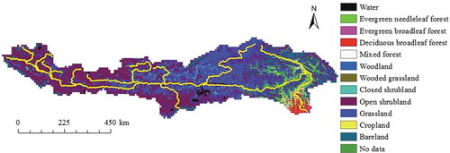
The VIC model was developed on a 1 km × 1 km grid. The baseline location information, including soil parameters, vegetation parameters and elevation data, was obtained as follows. The elevation dataset was downloaded from the Cold and Arid Regions Science Data Center at Lanzhou,² with a spatial resolution of 90 m × 90 m (Fig. 1). The types of land cover in the study area include herbaceous cover, snow and ice, needle-leaved evergreen vegetation, sparse shrub, bare soil, coniferous forest, broadleaf forest, cultivated and natural vegetation, water body, etc. (Fig. 2). The most widely distributed vegetation type is herbaceous cover, which accounts for over 60% of the area. In addition, the snow and ice, needle-leaved evergreen vegetation, and sparse shrub are sparsely distributed. Correspondingly, the required vegetation parameters, including the number of vegetation types, fraction rate, root distribution and monthly leaf area index (LAI) data, were collected from global land-cover datasets.³ In addition, soils were categorized according to the classification standard of the International Geosphere-Biosphere Program (IGBP) into Bulkdens, Sand and Clay. Soil parameters were obtained from the Food and Agriculture Organization Soil Map of the World.

Figure 1. Modelling grids and meteorological and hydrological stations in the YZRB.

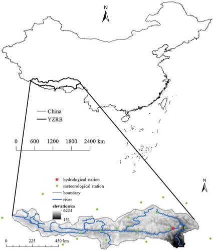
Figure 2. Vegetation of the YZRB.

Historical records of meteorological and hydrological data

Historical records of daily meteorological datasets were collected from the China Meteorological Data Service Center,⁴ including precipitation and air temperature (mean, maximum and minimum), for the period of 1961–2015 at 21 meteorological stations surrounding the study area (Fig. 1). Missing data have been treated by using a linear interpolation method (Yang et al. 2011). Daily discharge observation data for Nuxia station (Fig. 1) during 1961–2000, provided by the Hydrology and Water Resources Survey Bureau of the Tibet Autonomous Region, were used to calibrate model parameters and verify model performance. Nuxia station is located in the downstream and mainstream portions of the study area. In addition, daily surface soil moisture and surface soil temperature for the Southeastern Tibetan station (29.77°N, 94.74°E) from January 2007 to August 2013 were collected to evaluate the performance of VIC hydrological modelling.

Future meteorological data

The Fifth Report of the Intergovernmental Panel on Climate Change (IPCC⁵ ) provides recommended climate projections from more than 40 different global climate models. Relevant comparisons and assessments show that the Model for Interdisciplinary Research on Climate, fifth version (MIROC5) is capable of accurately capturing the spatial and temporal patterns of precipitation and air temperature in the study area (Kim et al. 2011, Mochizuki et al. 2012, Kumar et al. 2013, Liu et al. 2013, Huang et al. 2015, Qu et al. 2015, Yu et al. 2015). The MIROC5 datasets were produced by the Climate System Research Center of the University of Tokyo and the grid size of the datasets is 1.4° × 1.4°. Our previous analysis indicated that the MIROC5 dataset in GCM groups performed much better in the simulation of land meteorological variables (precipitation and temperature) in the YZRB (Liu et al. 2013). Outputs of MIROC5 for the period 2006–2100 and the historical records covering the period 1970–2005 were obtained from different climate scenarios (representative concentration pathways, RCP), i.e. RCP2.6, RCP6.0 and RCP8.5. According to previous studies, the differences between these climate scenarios come from radiation forcing levels of 2.6, 6.0 and 8.5 W/m², respectively. In terms of differences in their outputs, greater precipitation, higher temperature and bigger values for other meteorological factors are bound with higher radiation forcing levels, so more attention should be given to water resources management if the RCP8.5 scenario happens in the future, since such severe meteorological conditions would be mostly disadvantageous to future hydrological processes. Therefore, the MIROC5 RCP8.5 dataset was finally selected for further analysis.

Downscaling of meteorological variables

To match the model input data requirement, the downscaling method introduced by Immerzeel et al. (2012) was applied for downscaling the MIROC5 large-scale outputs to the required meteorological variables, including precipitation and air temperature (mean, maximum and minimum) for the 21 meteorological stations (Fig. 1) and corresponding grids. The downscaling method has been successfully applied in the Himalayan region. Below we describe the specific procedures of this method. First two adjustment coefficients are calculated with Equations (1) and (2), using the monthly averages and standard deviations, respectively, in both observations and MIROC5 datasets. Then, the monthly downscaled values are obtained from Equation (3):

(1) ${\mu }_m=\frac{\overline{x_{o,m}}}{\overline{x_{\mathrm{M}\mathrm{I}\mathrm{R}\mathrm{O}\mathrm{C}5,m}}}$(1)

(2) ${\sigma }_m=\frac{{\sigma }_{o,m}}{{\sigma }_{\mathrm{M}\mathrm{I}\mathrm{R}\mathrm{O}\mathrm{C}5,m}}$(2)

(3) $x_{\mathrm{M}\mathrm{I}\mathrm{R}\mathrm{O}\mathrm{C}5,m}^{\prime }=(x_{\mathrm{M}\mathrm{I}\mathrm{R}\mathrm{O}\mathrm{C}5,m}-\overline{x_{\mathrm{M}\mathrm{I}\mathrm{R}\mathrm{O}\mathrm{C}5,m}})\times {\sigma }_m+(x_{\mathrm{M}\mathrm{I}\mathrm{R}\mathrm{O}\mathrm{C}5,m}\times {\mu }_m)$(3)

where μ_m is the adjustment coefficient for averages; x_MIROC5,m, x′_MIROC5,m are the original and corrected meteorological values, respectively; and $\overline{x_{o,m}}$ and $\overline{x_{\mathrm{M}\mathrm{I}\mathrm{R}\mathrm{O}\mathrm{C}5,m}}$ are, respectively, the average observations and historical records from the period 1971–2005 for a given month, m (m = 1, …, 12, corresponding to January–December) of the MIROC5 datasets (either precipitation or temperature). Similarly, σ_m is the adjustment coefficient for standard deviation; and σ_o,_m and σ_MIROC5,m are the standard deviations of, respectively, the observations and the historical series in the MIROC5 datasets.

Next, the monthly-corrected MIROC5 datasets over 2006–2100 are disaggregated into daily values by using monthly allocations of the daily observations from 1970 to 2005. Specifically, the monthly sums are equal to the downscaled MIROC5 records, but the partitioning into daily values is based on the statistical distribution of the observations in the corresponding given months (January–December). In other words, daily allocation of different variables for a specific month is determined as the average daily rate in the specific month over 1970–2005 (for instance, the rate on 1 January in the total value for January is calculated as the average of the rate on 1 January in the total value for January of the years 1970–2005). This step outputs daily statistically downscaled precipitation and temperature for 2006–2100 at 21 meteorological stations, which are then used as the input forcing data of the calibrated VIC model. Spatial distribution in precipitation and temperature of the downscaled time series at all simulated pixels is obtained by using the kriging interpolation method (which has been validated by Hu et al. 2012 for the study area) in a GIS platform.

Model description

The VIC model was initially introduced by Liang (1994), and has been constantly developed through the improvement of partial algorithms and adding new modules: e.g. blowing snow algorithm, lake module, frozen soil calculation (Cherkauer and Lettenmaier 1999, Bowling et al. 2004, Gao et al. 2011). The VIC model is able to simulate soil–vegetation–atmosphere interactions on a large scale. It is characterized by consideration of the spatially varying infiltration capacity to represent sub-grid heterogeneity in soil parameters. With respect to runoff generation mechanisms, saturation excess runoff and infiltration excess runoff are simultaneously considered. More details regarding this model can be found online.⁶

Snow melting and accumulation processes were considered in our simulation. Liu et al. (2015) identified that seven soil-related parameters needed to be calibrated: the first, second and third soil-layer depths, the shape coefficient for the curve of variable infiltration capacity, the daily maximum groundwater runoff produced by soils, the ratio between groundwater runoff and the nondimensional parameter K_m when groundwater runoff shifts from linearity to nonlinearity, and the ratio between lower soil moisture and maximum soil moisture when groundwater runoff shifts from nonlinearity to linearity. For runoff generation, the VIC model considers both infiltration excess runoff and saturation excess runoff (Liu et al. 2012).

Parameter calibration and validation

To determine rational parameters of the VIC model in the case study, the shuffled complex evolution method developed at The University of Arizona (SCE-UA; Duan et al. 1994) was utilized for parameter calibration. The SCE-UA approach has been used as an effective evaluation method for the study area (Liu et al. 2015). The periods 1971–1980 and 1981–2000 were used as the calibration and validation periods, respectively. To validate the performance of the calibrated VIC model, the Nash-Sutcliffe coefficient of efficiency (E_NS) (Equation (4)), relative error (E_r) (Equation (5)), correlation coefficient (r), and coefficient of determination (R²) were all employed as the criteria for the assessment; for the calculation of r and R² refer to Liu et al. (2015). Larger values of E_NS, r, R², and a lower value of E_r indicate better performance of the model.

(4) $E_{\mathrm{N}\mathrm{S}}=1-\frac{\sum {(Q_{m,i}-Q_{o,i})}^2}{\sum {(Q_{o,i}-\overline{Q_o})}^2}$(4)

(5) $E_r=\frac{\sum Q_{m,i}}{\sum Q_{o,i}}-1$(5)

where $\overline{Q_o}$ refers to the monthly average of the observed streamflow in the period 1981–2000; Q_m,_i and Q_o,_i (i denotes rank of month during 1981–2000, i = 1, 2, …, 240) represent monthly observations and modelled streamflow at the Nuxia station, respectively.

Results of analysis

Performance of the downscaling model

The results of the comparison between observed precipitation and air temperature (mean, maximum and minimum) and downscaled series at 21 meteorological stations using the downscaling method are shown in Table 1 and Fig. 3. It is clear that the relative error (E_r) is generally less than 0.2 and the other calculated assessment indices, E_NS, R² and r, are over 0.6. Both these results show that the downscaling records agree well with observations in the study area.

Table 1. Comparison of the calibrated and uncalibrated series and the observed series in the calibration and validation periods.

Period	Series	Er	ENS	R^2	r
Calibration	Calibrated vs observed	–0.05	0.90	0.86	0.88
	Uncalibrated vs observed	–0.29	0.72	0.67	0.56
Validation	Simulated vs observed	–0.04	0.88	0.85	0.86

Figure 3. Performance of the downscaling model based on observations and the downscaled MICRO5 outputs. (a) Monthly precipitation, (b) monthly mean temperature, (c) monthly maximum temperature, (d) monthly minimum temperature.

Future precipitation projection

The percentage changes in precipitation at the annual scale are shown in Fig. 4(a–c). Specifically, for the period 2046–2060, precipitation in most regions would be less than corresponding values in 2006–2020, while the opposite is observed for the end of the century, especially in the central-southern regions, such as the Himalayan Mountains.

Figure 4. Precipitation in 2006–2020 and the variability in 2046–2060 and 2086–2100 in the YZRB. Note: The values in 2046–2060 and 2086–2100 refer to the variability: the variability in 2046–2060 was obtained by ((m_2046-2060 − m_2006-2020)/m_2006-2020), and the variability in 2086–2100 was ((m_2086-2100 − m_2046-2060)/m_2046-2060) (m_2006-2020, m_2046-2060 and m_2086-2100 are averages in hydrological elements during 2006–2020, 2046–2060 and 2086–2100, respectively).

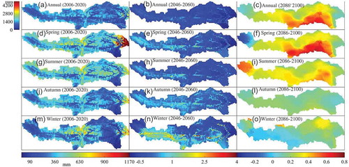
To recognize the seasonality in precipitation, the spatial distribution of seasonal precipitation for 2006–2020 and the variability of precipitation for 2046–2060 and 2086–2100 are displayed in Fig. 4(d–o). First, similarity is observed in the spatial patterns of variability between the periods 2006–2020 and 2046–2060 in spring and summer, in which a substantial decrease in precipitation is generally observed in the middle and eastern regions of the basin, while approximately half of the grids indicate increases and decreases in both spring and summer precipitation in the upstream region. As for autumn precipitation, most grids at the eastern edge of the basin still indicate an obvious decrease, while in other areas an increase in precipitation is dominant. In addition, a notable spatial discrepancy in the variability of winter precipitation is observed between the periods 2006–2020 and 2046–2060, in which there is a tendency of less decreasing precipitation on a number of grids, primarily concentrated in the northern area, compared to the other seasons.

Performance of the VIC model

In this study, the period 1961–1970 was used as a model spin-off. The period 1971–1980 was chosen for calibration, which was implemented by the SCE-UA method (Duan et al. 1994) on a monthly scale with the combination of monthly averaged streamflow at Nuxia hydrological station. The residual two decades, 1981–2000, were applied for model validation. The simulated streamflow at Nuxia station and the observations for 1971–1980 before and after model calibration using the SCE-UA method are compared in Fig. 5(a)). The correlation coefficient between observed series and simulated series improved to 0.88 after calibration (it was 0.56 before calibration), and larger values of E_NS and R² and a lower absolute value of E_r (0.90, 0.86 and 0.05, respectively), were obtained, which also illustrate that the calibrated method was effective. To verify the capability of the calibrated method, simulated streamflow and observations were compared for the period 1981–2000. The results demonstrate that the simulated series are in good agreement with the observed series, with r, E_NS, R² and E_r of 0.87, 0.88, 0.85 and −0.04, respectively, as shown in Fig. 5(b).

Figure 5. Performance of VIC model based on observations and the SCE-UA method: (a) streamflow at Nuxia station – calibration period; (b) streamflow at Nuxia station – validation period, (c) surface soil moisture at the Southeastern Tibetan station, (d) surface soil temperature at the Southeastern Tibetan station.

In addition, surface soil moisture and soil temperature at the Southeastern Tibetan station were also applied to verify the performance of the VIC model. Comparison between simulated and observed series was conducted on the monthly surface soil moisture (0–10cm) series for the Southeastern Tibetan station (Fig. 5(c)), and the matching extent was estimated by E_r, E_NS, R² and r, with values of −0.02, 0.80, 0.85 and 0.92, respectively, which reflects that good agreement is obtained in the simulation of surface soil moisture. Surface soil temperature was evaluated for the Southeastern Tibetan station (Fig. 5(d)), and the results for E_r, E_NS, R² and r between the simulated and observed series from January to December (–0.02, 0.86, 0.92 and 0.96, respectively) are also satisfactory. Thus, it is feasible to simulate the hydrological processes in the YZRB by using the calibrated VIC model.

Evapotranspiration

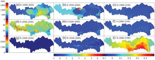
Regarding the spatial pattern in evapotranspiration (Fig. 6(a–c)) for the period 2006–2020, the magnitude of evapotranspiration in the upstream region is generally larger than that in the midstream and downstream regions, and the surrounding areas of the Himalayan Mountains have the largest evapotranspiration values over the entire basin. In the period 2046–2060, in contrast to 2006–2020, a substantial increase in evapotranspiration is found in the upstream region of the study area and a slight increase is detected in the midstream and downstream regions. Regarding the changes between the periods 2046–2060 and 2086–2100, no apparent variations in evapotranspiration are found over the entire basin, and rates of change range from approx. −10% to 10%.

Figure 6. Hydrological elements during 2006–2020, and their percentage differences between 2046–2060 and 2006–2020 as well as between 2086–2100 and 2046–2060 in the YZRB. Note: E, S and R in the figure represent evapotranspiration, soil moisture and runoff depth, respectively.

For the period 2006–2020, the seasonal mean evapotranspiration is compared in Fig. 7, in which the values in summer are comparatively large over most of the area. However, with respect to the variability of summer evapotranspiration between the periods 2006–2020 and 2046–2060, an overall decrease in evapotranspiration is observed, except for a few grids in the upstream region. A similarity is observed between the variability in spring and winter evapotranspiration and an overall increase is identified for both, in which the only difference is exhibited at the northwestward edge of the basin, where an increase and a decrease are detected in spring and winter evapotranspiration, respectively. As for the autumn evapotranspiration, the magnitude is less than the corresponding summer evapotranspiration for the period 2006–2020, and the spatial pattern of variability for the period 2046–2060 generally indicates an increase in evapotranspiration over the entire basin.

Figure 7. Seasonal evapotranspiration in 2006–2020 and the variability in 2046–2060 and 2086–2100 in the YZRB.

Inspection of the variability in seasonal evapotranspiration between the periods 2046–2060 and 2086–2100 suggests a slight increase in spring and summer evapotranspiration, only the northeastern areas having decreasing summer evapotranspiration. For the autumn evapotranspiration, an overall decrease in the grids at the northwestward edge of the basin, midstream and downstream is observed. However, a general increase is observed in the seasonal evapotranspiration.

Soil moisture

In contrast to evapotranspiration, soil moisture (Fig. 6(d–f)) in the upstream section is projected as a slight reduction at an annual scale in the period 2046–2060 compared to 2006–2020. In the midstream and downstream, most areas have a slight increase in soil moisture. Comparably larger changes are observed in the southeastern corner of the YZRB and in part of the Nianchu River basin. The differences in soil moisture between the periods 2046–2060 and 2086–2100 are similar to those for evapotranspiration; specifically, increases are identified for most pixels in the study area and a few pixels in the downstream northeastern corner are projected to have decreases in soil moisture.

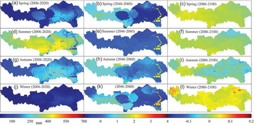
Regarding seasonal soil moisture in the study area (Fig. 8), the spatial patterns for the period 2006–2020 are markedly consistent over all seasons, with the following ascending rank of values: winter, spring, autumn and summer. Similarly, regarding the variability in seasonal soil moisture, the spatial patterns over all seasons are also in agreement, where decreases in soil moisture are observed in the upstream in spring, and grids in the upstream and midstream decrease in summer and autumn. Correspondingly, grids in the midstream and downstream areas increase in summer and autumn. Moreover, increases in soil moisture in winter are generally distinguished over the entire basin, which is opposite to the value ranking of seasons listed above. Regarding the variability of soil moisture between the periods 2046–2060 and 2086–2100, no overall substantial decrease in seasonal soil moisture is projected. The variability in winter soil moisture is most extensive over different seasons.

Figure 8. Seasonal soil moisture in 2006–2020 and the variability in 2046–2060 and 2086–2100 in the YZRB.

Runoff

The spatial pattern of annual runoff over the study area (Fig. 6(g–i)) for the period 2006–2020 is in good agreement with that of annual precipitation. The annual runoff decreases over the entire basin from 2006–2020 to 2046–2060, while it increases from 2046–2060 to 2086–2100.

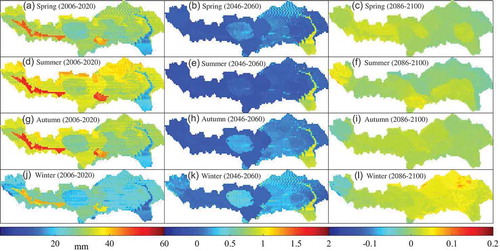
There is an apparent inconsistency in the variability of seasonal runoff (Fig. 9) between 2006–2020 and 2046–2060, in which summer runoff substantially increases over the majority of the basin, and the magnitude of the increases develops from upstream to downstream. There is also an apparent inconsistency in the spatial pattern of winter runoff at the uppermost edge of basin, in which substantial increases in runoff are identified. Slight increases are observed in the upstream and part of the midstream of the basin, with slight increases in runoff during winter. Decreases in runoff are generally monitored downstream. Decreases in runoff are also observed in spring and autumn over the majority of the basin.

Figure 9. Seasonal runoff depth in 2006–2020 and the variability in 2046–2060 and 2086–2100 in the YZRB.

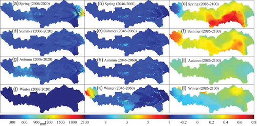
For the period between 2046–2060 and 2086–2100, seasonal runoff in most areas of the basin is projected to increase, and the variability of spring and summer runoff is dominant. Specifically, increases in autumn runoff are generally inconspicuous and similar results are discovered in winter runoff, while differentiated increases appear in winter runoff at the northeastern areas of the study area. In addition, a spatial discrepancy in the variability of spring runoff could be observed, in which runoff in several grids in the northwestern areas apparently decreases, while in other areas it generally increases, and the larger increases occur in the Nianchu River basin (27.92°N–29.34°N, 88.58°E–90.16°E) and the Himalayan Mountains (29.63°N–31.29°N, 74.59°E–95.06°E). Smaller increases are observed in summer runoff, and substantial increases in runoff are evident at the northwestward edge of the basin and the Big Bend region.

Discussion

All the variability in the selected hydrological elements between the periods 2006–2020 and 2046–2060, as well as between 2046–2060 and 2086–2100 indicate notable consistency at both annual and seasonal scales. Specifically, decreases are generally identified for the period between 2006–2020 and 2046–2060 at various time scales, except for evapotranspiration, while in winter, all the hydrological elements increase. Comparatively substantial increases in precipitation and runoff are recognized between 2046–2060 and 2086–2100. The variability in evapotranspiration and soil moisture is less evident; specifically, increases in evapotranspiration are observed, and the changes in soil moisture are consistent with those of precipitation and runoff. Similar results were also obtained in previous studies: e.g. both Ma et al. (2010) and Shi et al. (2013) noted that downstream runoff of Himalayan catchments will decrease in the near future, but in the long run, increased runoff will occur. Similarly to this study, a slight decrease in downstream runoff for the Himalayan catchments was projected up to the 2050s, and then a significant decrease in the streamflow should be experienced till at least the end of the 21st century.

The results of this study illustrate that runoff variations are mainly due to precipitation changes in terms of both magnitude and variability at various time scales. Regarding the seasonality in runoff, acceleration in runoff caused by the melting of snow, glaciers and frozen soils is a result of the increase in air temperature, which is another driver for runoff increases. Similar conclusions were found in previous studies. Xuan and Xu (2017) demonstrated a continuous influence of precipitation on runoff, while the impacts of snowmelt runoff on out-runoff exist during summer. Immerzeel et al. (2012) described how increases in rainfall runoff and baseflow induced by glacier reduction would result in increases in river flow over the glacier catchment of the Himalayas. Moreover, increases in evapotranspiration were detected between the periods 2006–2020 and 2046–2060, with increases in the upstream areas and decreases in midstream and downstream areas between the periods 2046–2060 and 2086–2100. However, Shi et al. (2013) maintained that decreased evapotranspiration would occur. Discrepancies in the variability of evapotranspiration in this study compared to previous studies could be attributed to the datasets included and relevant algorithms in the models.

Great uncertainty remains in the projection of future climate information. In terms of the analysis in this study, three RCP scenarios have notable discrepancies in the output datasets. Two of them, RCP2.6 and RCP6.0, were found to have no available data in the study area. Besides, the missing data in the observations may affect the effectiveness of calibration to a certain extent. In addition, the common problems in parameter optimization, e.g. different parameter sets may reach consistent results, remain in our study, which could lead to misunderstandings of the physically-based parameters in the case study. Therefore, increasing the accuracy of data and the improvement of relevant methods should be the focus of future study.

Conclusions

Hydrological processes from 1981 to 2100 were simulated using the VIC hydrological model in combination with the CMIP5 and MIROC RCP8.5 datasets and other required datasets. The performance of the VIC model, the downscaling method and the SCE-UA method was assessed, and hydrological processes in the periods 2006–2020, 2046–2060 and 2086–2100 were extracted and analysed for the entire YZRB. The results can be summarized as follows.

The VIC model, the downscaling method and the SCE-UA method are suitable for the study area.

The variability in evapotranspiration and soil moisture is relatively small, and increases in annual evapotranspiration are indicated between the periods 2006–2020 and 2046–2060 over the entire basin. Increases in soil moisture in upstream areas and decreases in midstream and downstream areas are also indicated. For the period 2086–2100, both evapotranspiration and soil moisture present slight increases in upstream and midstream areas, and slightly decreases are found in downstream areas.

Between the periods 2006–2020 and 2046–2060, annual precipitation, soil moisture and runoff all decrease, and both annual precipitation and runoff have substantial increases between the periods 2046–2060 and 2086–2100, especially in the Himalayan Mountains and Nianchu River basin.

Substantial increases in precipitation and runoff in spring and summer are generally observed between the periods 2046–2060 and 2086–2100, especially in the Himalayan Mountains. The variability in precipitation might be the predominant factor influencing runoff in the YZRB.

Acknowledgements

The authors extend their thanks to the reviewers for their careful comments which helped to improve the paper.

Disclosure statement

No potential conflict of interest was reported by the authors.

Additional information

Funding

This study is financially supported by the State Key Program of the Natural Science Foundation of China (NSFC) [91647202]. We fully acknowledge the support received from the Open Fund Research project by the State Key Laboratory of Hydraulics and Mountain River Engineering (Sichuan University) [SKHL1709].

Notes

¹ https://esgf-node.llnl.gov/projects/cmip5/.

² http://westdc.westgis.ac.cn.

³ http://www.landcover.org/data/landcover/data.shtml.

⁴ http://data.cma.cn/.

⁵ https://www.ipcc.ch/assessment-report/ar5/.

⁶ http://github.com/UW-Hydro/VIC.

References

- Beldring, S., 2002. Multi-criteria validation of a precipitation–runoff model. Journal of Hydrology, 257 (1), 189–211. doi:10.1016/S0022-1694(01)00541-8
- Bowling, L.C., Pomeroy, J.W., and Lettenmaier, D.P., 2004. Parameterization of blowing snow sublimation in a macroscale hydrology model. Journal of Hydrometeorology, 5 (5), 745–762. doi:10.1175/1525-7541(2004)005<0745:POBSIA>2.0.CO;2
- Chen, Y.N., et al., 2006. Regional climate change and its effects on river runoff in the Tarim basin, China. Hydrological Processes, 20, 2207–2216. doi:10.1002/(ISSN)1099-1085
- Cherkauer, K.A. and Lettenmaier, D.P., 1999. Hydrologic effects of frozen soils in the upper Mississippi River basin. Journal of Geophysical Research, 104 (D16), 19599–19610. doi:10.1029/1999JD900337
- Collins, D.N., 2008. Climatic warming, glacier recession and runoff from Alpine basins after the Little Ice Age maximum. Annals of Glaciology, 48 (48), 119–124. doi:10.3189/172756408784700761
- Dong, L.X., et al., 2009. The change of land cover and land use and its impact factors in upriver key regions of the Yellow River. International Journal of Remote Sensing, 30 (5), 1251–1265. doi:10.1080/01431160802468248
- Duan, Q., Sorooshian, S., and Gupta, V.K., 1994. Optimal use of the SCE-UA global optimization method for calibrating watershed models. Journal of Hydrology, 158 (3–4), 265–284. doi:10.1016/0022-1694(94)90057-4
- Gao, H., et al., 2011. On the causes of the shrinking of Lake Chad. Environmental Research Letters, 6, 034021. doi:10.1088/1748-9326/6/3/034021
- Gao, X.Y., et al., 2015. Soil salt and groundwater change in flood irrigation field and uncultivated land: a case study based on 4-year field observations. Environmental Earth Sciences, 73 (5), 2127–2139. doi:10.1007/s12665-014-3563-4
- Gouttevin, I., et al., 1994. Multi-scale validation of a new soil freezing scheme for a land-surface model with physically-based hydrology. Cryosphere Discussions, 6 (2), 2197–2252.
- Hu, L.J., et al., 2012. Spatial interpolation of meteorological variables in Yarlung Zangbo River basin. Journal of Beijing Normal University (natural Science Edition), 48 (5), 449–452. (in Chinese).
- Huang, Y., Li, X., and Wang, H., 2015. Will the western Pacific subtropical high constantly intensify in the future? Climate Dynamics, 47 (1–2), 1–11.
- Immerzeel W.W., et al., 2012. Hydrological responses to climate change in a glacierized catchment in the Himalayas. Climatic Change, 110, 721–736. doi:10.1007/s10584-011-0143-4
- Jayawickreme, D.H. and Hyndman, D.W., 2007. Evaluating the influence of land cover on seasonal water budgets using Next Generation Radar (NEXRAD) rainfall and streamflow data. Water Resources Research, 43 (2), 604–614. doi:10.1029/2005WR004460
- Kim, H.J., et al., 2011. Global monsoon, El Niño, and their interannual linkage simulated by MIROC5 and the CMIP3 CGCMs. Journal of Climate, 24 (21), 5604–5618. doi:10.1175/2011JCLI4132.1
- Kumar, S., et al., 2013. Land use/cover change impacts in CMIP5 climate simulations: a new methodology and 21st century challenges. Journal of Geophysical Research, 118 (3), 6337–6353.
- Li, F., et al., 2012. Changes of land cover in the Yarlung Tsangpo River basin from 1985 to 2005. Environmental Earth Sciences, 68 (1), 181–188. doi:10.1007/s12665-012-1730-z
- Liang, X., 1994. A two-layer variable infiltration capacity land surface representation for general circulation models. Thesis (PhD). University of Washington.
- Liu, W.F., et al., 2012. Distributed hydrological simulation in the Lhasa River basin based on VIC model. Journal of Beijing Normal University (natural Science), 48 (5), 524–529. (in Chinese).
- Liu, W.F., et al., 2013. GCM performance on simulating climatological factors in Yarlung Zangbo River basin based on a ranked score method. Journal of Beijing Normal University (natural Science), 49 (2/3), 304–311. (in Chinese).
- Liu, W.F., et al., 2015. Impacts of climate change on hydrological processes in the Tibetan Plateau: a case study in the Lhasa River basin. Stochastic Environmental Research and Risk Assessment, 29 (7), 1809–1822. doi:10.1007/s00477-015-1066-9
- Liu, Z.F., et al., 2010. Impacts of climate change on hydrological processes in the headwater catchment of the Tarim River basin, China. Hydrological Processes, 24 (2), 196–208.
- Ma, X., Xu, J.C., and Noordwijk, M.V., 2010. Sensitivity of streamflow from a Himalayan catchment to plausible changes in land cover and climate. Hydrological Processes, 24, 1379–1390. doi:10.1002/hyp.v24:11
- Mochizuki, T., et al., 2012. Decadal prediction using a recent series of MIROC global climate models. Journal of the Meteorological Society of Japan, 90A (2), 373–383. doi:10.2151/jmsj.2012-A22
- Osborn, H.B. and Lane, L., 1969. Precipitation–runoff relations for very small semiarid rangeland watersheds. Water Resources Research, 5 (2), 419–425. doi:10.1029/WR005i002p00419
- Ouyang, F., et al., 2015. Impacts of climate change under CMIP5 RCP scenarios on streamflow in the Huangnizhuang catchment. Stochastic Environmental Research & Risk Assessment, 29 (7), 1781–1795. doi:10.1007/s00477-014-1018-9
- Pan, F. and King, A.W., 2012. Downscaling 1-km topographic index distributions to a finer resolution for the TOPMODEL-based GCM hydrological modeling. Journal of Hydrologic Engineering, 17 (2), 243–251. doi:10.1061/(ASCE)HE.1943-5584.0000438
- Qu, X., et al., 2015. Equatorward shift of the South Asian high in response to anthropogenic forcing. Theoretical & Applied Climatology, 119 (1–2), 113–122. doi:10.1007/s00704-014-1095-1
- Seibert, J., 1999. Regionalisation of parameters for a conceptual rainfall–runoff model. Agricultural and Forest Meteorology, 98–99, 279–293. doi:10.1016/S0168-1923(99)00105-7
- Shi, P., et al., 2013. Effects of land-use and climate change on hydrological processes in the upstream of Huai River, China. Water Resource Management, 27 (5), 1263–1278. doi:10.1007/s11269-012-0237-4
- Speak, A.F., et al., 2013. Rainwater runoff retention on an aged intensive green roof. Science of the Total Environment, 461-462 (7), 28–38. doi:10.1016/j.scitotenv.2013.04.085
- Ullrich, A. and Volk, M., 2009. Application of the Soil and Water Assessment Tool (SWAT) to predict the impact of alternative management practices on water quality and quantity. Agricultural Water Management, 96 (8), 1207–1217. doi:10.1016/j.agwat.2009.03.010
- Valdés, J.B., Seoane, R.S., and North, G.R., 2015. A methodology for the evaluation of global warming impact on soil moisture and runoff. Journal of Hydrology, 161 (1–4), 389–413. doi:10.1016/0022-1694(94)90137-6
- Wu, Z.Y., et al., 2007. Thirty-five year (1971–2005) simulation of daily soil moisture using the variable infiltration capacity model over China. Atmosphere, 45 (1), 37–45.
- Xuan, W.D. and Xu, Y.P., 2017. Runoff projection under climate change over Yarlung Zangbo River, Southwest China. EGU, 19, 16479.
- Xue, B.L., et al., 2013. Modeling the land surface water and energy cycles of a mesoscale watershed in the central Tibetan Plateau during summer with a distributed hydrological model. Journal of Geophysical Research Atmospheres, 118, 8857–8868.
- Yang, Z., Liu, Y., and Li, C., 2011. Interpolation of missing wind data based on ANFIS. Renewable Energy, 36 (3), 993–998. doi:10.1016/j.renene.2010.08.033
- Yu, E.T., et al., 2015. Evaluation of a high-resolution historical simulation over China: climatology and extremes. Climate Dynamics, 45, 2013–2031. doi:10.1007/s00382-014-2452-6
- Zhang, Y., et al., 2018. Characterizing drought in terms of changes in the precipitation–runoff relationship: a case study of the Loess Plateau, China. Hydrology and Earth System Sciences, 22 (3), 1749–1766. doi:10.5194/hess-22-1749-2018
- Zhu, Q.A., et al., 2012. Effects of future climate change, CO2 enrichment, and vegetation structure variation on hydrological processes in China. Global and Planetary Change, 80 (1), 123–135. doi:10.1016/j.gloplacha.2011.10.010