Reconstruction of groundwater levels to impute missing values using singular and multichannel spectrum analysis: application to the Ardabil Plain, Iran

ABSTRACT

Groundwater-level time series often have a substantial number of missing values which should be taken into consideration before using them for further analysis, particularly for numerical groundwater flow modelling applications. This study aims to comprehensively compare two data-driven models, singular spectrum analysis (SSA) and multichannel spectrum analysis (MSSA), to reconstruct groundwater-level time series and impute the missing values for 25 piezometric stations in Ardabil Plain, northwest Iran. The reconstructed groundwater-level time series are assessed against the complete observed groundwater time series, while the imputed values are appraised against the artificially created gap values. The results show that both SSA and MSSA demonstrate a solid competency in imputation and reconstruction of groundwater-level data. However, depending on the spatial correlation between the piezometers, and the most suitable probability distribution function (pdf) fitted to the time series of each piezometer, the performance may vary from piezometer to piezometer.

KEYWORDS:

• groundwater-level time series
• imputation of missing values
• reconstruction of groundwater level
• singular and multichannel spectrum analysis
• Iran

Editor S. Archfield Associate editor F.-J. Chang

1 Introduction

There is a worldwide consensus that groundwater is generally one of the most important sources for drinking water and irrigation (Lachaal et al. 2011, Mohammadi et al. 2014, Jellalia et al. 2015, Thomas and Famiglietti 2015, Zaidi et al. 2015, Asfahani 2016). Therefore, successful water resources management is strongly dependent on sustainable groundwater resources management (Amer et al. 2012, Palazzo and Brozovic 2014, Wu et al. 2016). However, to manage water resources appropriately requires the availability of long-term and high-quality groundwater data recorded at different spatial and temporal scales (Khalil et al. 2001, Zhou et al. 2013).

To get a more or less continuous shape of a groundwater table, point-measured piezometric heads in an aquifer are usually interpolated and/or extrapolated through various geostatistical methods, whereby, depending on the method, the influence of neighbouring piezometers on the computed head in question may vary significantly. This means that a lack of information at a given piezometer may result in a severe distortion of the shape of the computed groundwater table (Dax 1985, Walker et al. 2016). The same is true in the presence of erroneous data: it is important to remove and to substitute suspicious data by imputed values (Alley et al. 1999, Harvey et al. 2012).

When applying numerical groundwater models, the observed water levels are usually used in the calibration process and/or for setting initial and boundary conditions. To do so, the point-measured groundwater-level data are transferred onto a mesh of cells, or elements of the discretization of the numerical model. Hence, missing observations can seriously affect the input to such a model (Walczak and Massart 2001, Nkiaka et al. 2016). Additionally, it is well known that many poorly set-up groundwater models are quite unstable or ill-posed, which means that small changes in the input data and/or initial and boundary conditions may lead to large variations in the values of the targeting parameters in the calibration (i.e. the inversion process). This demonstrates, therefore, that missing (or erroneous) observations can produce large errors in the output of a model (Dax 1985).

A lack of data ensues from a variety of factors, such as temporary absence of observers, damaged monitoring equipment, or lack of financial resources (Gyauboakye and Schultz 1994, Adeloye 1996, Teegavarapu et al. 2009). To cope with this problem, an important pre-processing operation, so-called “data refinement” should be carried out (Adeloye 1996, Adeloye et al. 2011, Mwale et al. 2012). In this regard, “gap” values are tackled either by eliminating the vectors containing missing samples, or by simply using some mean or zero substitution. Correspondingly, these types of refinement lead to the loss of a lot of information in most cases and, as such, they should not be considered (Gill et al. 2007). Preferably, dealing with the missing data problem in some fashion is encouraged, although reproducing missing data might be an unpleasant and tedious task (Ball 2003). Nonetheless, it is imperative that it is conducted carefully and as accurately as possible, because poor imputing of missing values may result in poor decisions being made (Benzvi and Kesler 1986, Bardossy and Pegram 2014).

Missing data handling approaches can be classified in two broad classes: the first includes techniques that are based on discarding a portion of the sample, such as listwise deletion (e.g. Dixon 2008) and pairwise deletion (e.g. McKnight et al. 2008), while the second class includes approaches that replace missing data with imputed values (e.g. Cheema 2014). Concerning the imputation approaches, a wide range of techniques have been developed, such as: marginal mean imputation (e.g. Allison 2001); regression approaches (e.g. Liu et al. 2018); autoregressive model imputation (e.g. Bashir and Wei 2018); maximum likelihood expectation-maximization (EM) imputation (e.g. Kim et al. 2011); multiple imputation method (e.g. Liu et al. 2019); hot deck technique (e.g. Srebotnjak et al. 2012); dummy variable adjustment approach (e.g. Jones 1996); zero imputation (e.g. McKnight et al. 2008); single random imputation (e.g. Zhang 2016); and last observed value carried forward (LOCF) model (e.g. Lachin 2016).

Depending on the time series’ lengths, frequency and periods of gaps, availability of neighbouring data, period of the knowledge, expertise of the person dealing with the missing data, and physical conditions of the study area, one of the aforementioned techniques may be employed to impute gap values (Gyauboakye and Schultz 1994, WMO 2008, Harvey et al. 2012). However, amongst the statistical methods, regression models can only be applied to reconstruct the data in cases where predictors are not missing (Adeloye 2009, Kim and Pachepsky 2010). Additionally, classical regression models typically analyse for one predictand (or dependent variable), so that for a large number of variables, the necessary creation of different predictive regression equations may be time-consuming (Wosten et al. 2001, Miller 2011). Furthermore, when there are substantial continuous missing values, conventional gap-filling techniques, including regression and geostatistical methods, such as kriging or inverse distance weighting (IDW), which are dependent on the availability of some neighbouring predictor variables, are not applicable (Teegavarapu and Chandramouli 2005, Dumedah and Coulibaly 2011).

The above-mentioned limitations of traditional approaches to imputing missing values have provoked a great deal of attention to data-driven models. Amongst these, singular spectrum analysis (SSA) and multi-channel singular spectrum analysis (MSSA) have recently gained popularity (Golyandina and Korobeynikov 2014). The main concept behind SSA is the decomposition of the series of interest into several segments, which can be classified as trends, oscillatory and noise components (Loève 1977, Golyandina et al. 2001, Rodrigues and de Carvalho 2013, Golyandina and Korobeynikov 2014). The SSA approach essentially extracts information from short and noisy time series without prior knowledge of the dynamics affecting the time series (Vautard and Ghil 1989, Schoellhamer 2001). Both SSA and MSSA are based on the singular value decomposition (SVD) of a certain matrix created using the time series. Neither a parametric model nor stationarity-type conditions are required to be assumed for the time series. This makes these high-skill, data-driven techniques model-free and thus enables SSA and MSSA to have a very wide range of uses (Golyandina and Zhigli︠a︡vskiĭ 2013). Moreover, compared with autoregressive (AR) models, SSA does not demand a priori model for trend or a priori knowledge of the number of periodicities and period values. Also, periodicities can be adjusted in different ways and hence, the type of model – additive or multiplicative – is not essential to be taken into account (Hassani et al. 2009).

The SSA and MSSA approaches have been applied mainly for gap filling and short- and long-term forecasting in the fields of meteorology, hydrology and Earth sciences, such as: gap filling of sediment concentration (Schoellhamer 2001, Shen et al. 2015); streamflow data imputation (Kondrashov et al. 2005, Agac et al. 2015); filling in missing MODIS (Moderate Resolution Imaging Spectroradiometer) land products (Kandasamy et al. 2013); gap filling of solar wind and interplanetary magnetic field data (Kondrashov et al. 2010); 3D seismic data de-noising and reconstruction (Rekapalli et al. 2017); short-term point and interval forecasts of daily maximum tropospheric ozone concentrations (Hansen and Noguchi 2017); wind speed forecasting (Moreno and dos Santos Coelho 2018); and simulation of water infiltration rate in response to a wide range of suspended solid sizes and concentrations (Taie Semiromi and Ghasemian 2018). Nevertheless, to the best of our knowledge, no reference study to date has applied SSA and MSSA to impute missing values in groundwater-level data.

Thus, the objectives of this paper are firstly, to assess the performance of SSA and MSSA in the imputation of “missing values” of 25 piezometric stations located in the Ardabil Plain aquifer, Iran, especially for the period December 1988 to March 1989 when no measurements are available. To that end, artificial missing values are created in a random manner, thereby allowing us to appraise the skill of SSA and MSSA against the observed values (the original values before being artificially removed). Secondly, we compare the competency of SSA and MSSA for reconstruction of the complete time series of 25 piezometric stations.

The study area and the piezometric datasets used are presented in Sections 2 and 3, respectively. In Section 4, the data analysis methodology, i.e. the SSA- and MSSA-formulation for a continuous time series and the gap-filling procedure is discussed. In Section 5, we present the results of the application of SSA and MSSA to fill in gaps in the piezometric time series. We conclude with a summary of the results in Section 6.

2 Study area

Ardabil Plain aquifer (38°30ʹ–38°27ʹN; 47°55ʹ–48°20ʹE), in northwest Iran, extends over an area of 1073 km² (Fig. 1(a)). There are two high mountain ranges, Alborz and Sabalan, which surround the Ardabil aquifer. The mean areal annual precipitation in the region amounts to 304 mm, with May and August being the wettest and driest months of the year, respectively (Ardabil Regional Water Authority 2013, Nourani et al. 2015). With an average annual temperature of only 9°C, the Ardabil aquifer is known to be one of the coldest regions in Iran, as also witnessed by an average of 130 freezing days in a year (Vousoughi et al. 2013).

Figure 1. (a) Geographical location of Gharehsoo River Basin (GRB) in Iran; (b) geological map of the basin and Ardabil aquifer, (c) and geographical distribution of the selected piezometers on Ardabil aquifer.

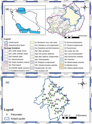
Geologically, the Ardabil plain was formed from Quaternary alluvial deposits which originate from the erosion and alteration of the surrounding mountains (Fig. 1(b)). Based on the results of geophysical exploration and drilling logs, the aquifer has a thickness varying from 10 m to more than 200 m and is mainly composed of gravel, sand and a small amount of clay. In accordance with pumping tests conducted over the aquifer, the transmissivity of the latter ranges from 50 to 2200 m²/d and the specific yield from 0.021 to 0.14. The dominant direction of groundwater flow is toward the northwest of the plain (Kord and Asghari Moghaddam 2014).

Demographically, based on the national census taken in 2011, 564 000 people live in the Ardabil Plain, inhabiting two major cities and 88 villages (Statistical Center of Iran 2011). Agriculture makes up the principal occupation of the inhabitants in the area. Since 1980, the rapid expansion of Ardabil city, intense agricultural activity, and some industrial activities have caused great stress on the Ardabil aquifer, as the average annual water consumption for the drinking, industrial and agricultural sectors amounts to 26, 4 and 177 × 10⁶ m³/year), respectively, with 89% of this water supplied from groundwater (Ardabil Regional Water Authority 2013). The groundwater is supplied through 2622 active pumping wells, 36 qanats and 77 springs operating across the Ardabil Plain (Kord and Asghari Moghaddam 2014).

3 Groundwater-level datasets

In this study, monthly piezometric data from 25 observation wells/piezometers distributed over the Ardabil plain are considered (Fig. 1(c)). These groundwater-level data, recorded from June 1988 to the end of 2013, result – theoretically – in 307 discrete observations. However, the groundwater-level time series have missing data as a result of: (a) destruction and plugging of piezometers owing to flooding; (b) curiosity of the local people, leading to destruction of wells; (c) inaccessibility of piezometers in stormy and snowy weather, particularly during winters; (d) defective water-level meters and lack of financial resources for repair and renewal; and (e) complete drying-up of piezometers leading to failure to determine the groundwater level. Above all, for unknown reasons, no groundwater levels were available in any of the 25 piezometers for the period December 1988–March 1989. Table 1 lists the statistics of the data for each well and indicates that piezometers P56 and P46/P19 have the maximum and minimum number of gaps in their data series, respectively.

Table 1. Statistics of the piezometric stations with number and percentage of missing data for each piezometer, ordered from maximum to minimum.

Piezometer	N valid	Missing		Mean	Std. dev.
		N	%
P56	189	118	38.40	1319.13	13.64
P16	208	99	32.20	1335.61	1.25
P37	224	83	27.00	1432.29	1.57
P15	226	81	26.40	1330.30	0.88
P55	233	74	24.10	1314.69	1.86
P23	239	68	22.10	1314.90	2.03
P18	245	62	20.20	1333.60	4.95
P28	251	56	18.20	1381.74	0.57
P27	258	49	16.00	1417.11	1.81
P36	261	46	15.00	1359.75	5.22
P8	261	46	15.00	1336.08	2.00
P13	262	45	14.70	1322.28	1.83
P31	268	39	12.70	1315.43	8.60
P25	271	36	11.70	1335.46	4.30
P20	271	36	11.70	1313.80	1.89
P35	273	34	11.10	1308.31	1.55
P17	276	31	10.10	1361.94	0.49
P53	280	27	8.80	1355.20	8.63
P10	280	27	8.80	1370.04	0.38
P5	283	24	7.80	1304.05	1.45
P51	287	20	6.50	1313.61	10.51
P38	289	18	5.90	1316.00	6.65
P44	291	16	5.20	1317.12	0.59
P46	292	15	4.90	1436.85	2.45
P19	292	15	4.90	1304.97	0.67

Std dev.: standard deviation.

In this study, to identify how missing and non-missing values are distributed, the distribution, pattern and frequency of missing data were evaluated (shown in the Supplementary material, Figs. S1–S3). A missing data pattern refers to the configuration of observed and missing values in a dataset (Enders 2010). To create such a pattern chart, the variables are first ordered from left to right in increasing order of missing values. Patterns are then sorted by the last variable (non-missing values first, then missing values), and then, by the second-to-last variable, and so on, working from right to left. This reveals whether the monotone imputation method can be used for the data, or, if not, how closely the data approximate to a monotone pattern.

4 Methodology

4.1 SSA

In this section, the outlines of the SSA and MSSA are explained and the procedure for reconstructing the groundwater-level series with temporal gaps is described. The primary objective of a SSA analysis is to decompose a time series into trend, cyclical, seasonal and noise by means of an eigen-decomposition of the so-called trajectory matrix (Khan and Poskitt 2013, Taie Semiromi and Ghasemian 2018).

To provide an accurate identification of the trends and seasonal periodicities (oscillations) in the groundwater-level series, analyses of the graphs of eigenvalues and eigenvectors of the elementary components of the SSA decomposition are of paramount importance (Golyandina and Korobeynikov 2014) (see Supplementary material, Figs. S4–S7). More specifically, these time series components can be identified through inspection of the shape of an eigenvector imitating the shape of the time series component that produces this eigenvector.

In the light of this decomposition, the initial/original time series can be reconstructed (Fig. S5) up to a desired accuracy by adopting five consecutive methodological schemes: (a) embedding; (b) singular value decomposition (SVD); (c) eigentriple grouping; (d) diagonal averaging; and (e) gap filling, as described briefly in the subsequent sub-sections.

4.1.1 Embedding

Assuming a real time series X = (x₁, …, x_N) of length N and an integer number L (1 < L < N), defining a possible window length, to conduct the embedding, the initial time series is projected onto a sequence of lagged vectors of size L by creating K = N − L + 1 lagged vectors X_i (i = 1, ., K) which may be put together to form a trajectory matrix defining a one-to-one correspondence between the trajectory matrix of size L × K and the original time series:

(1) $\mathit{X}=\left[X_1:\dots :X_K\right]={\left(X_{ij}\right)}_{i,j=1}^{L,K}=\left(\begin{array}{ccccc}{x}_1& x_2& x_3& \cdots & x_K\\ x_2& x_3& x_4& \dots & x_{K+1}\\ x_3& x_4& x_5& \dots & x_{K+2}\\ ⋮& ⋮& ⋮& \ddots & ⋮\\ x_L& x_{L+1}& x_{L+2}& \cdots & x_N\end{array}\right)$(1)

This matrix has two main characteristics: (a) the rows and columns of X are subseries of the original time series, and (b) X has equal elements on anti-diagonals, i.e. it is a Hankel matrix. In both SSA and MSSA applications, the window length L should be chosen appropriately to ensure that each L-lagged vector includes an essential part of the behaviour of the original series X = (x₁, …, x_N). Usually L is determined as L = N/2 by default, but by varying L, the dynamics of certain properties of the time series can be investigated (Golyandina and Zhigli︠a︡vskiĭ 2013), as will be demonstrated later in the applications.

4.1.2 Singular value decomposition (SVD)

In the second step, a singular value decomposition (SVD) of the trajectory matrix X, or, more specifically, of the correlation matrix C = XX^T, is made, i.e. X can be written as X = U S^1/2 V^T, where U and V are the left and right singular vectors and S^1/2 is the diagonal matrix of the singular values of X, equal to the eigenvalue matrix S of C = XX^T in decreasing order, λ₁ ≥ ··· ≥ λ_L ≥ 0. With the SVD, X can be reconstructed as:

(2) $\mathit{X}={\sum }_i\sqrt{{\lambda }_i}{U}_i{V}_i^T={\mathit{X}}_1+\dots +{\mathit{X}}_L$(2)

The triple ($\surd$λ_i, U_i, V_i) is called ith eigentriple (ET) (Golyandina and Zhigli︠a︡vskiĭ 2013, Golyandina and Korobeynikov 2014).

4.1.3 Eigentriple grouping

Based on the expansion (2), a separation of additive components of the original time series by a so-called eigentriple grouping is performed, by dividing a set of indices {1, …, d} with d = max{j: λ_j ≠ 0} into m disjoint subsets I₁, …, I_m, i.e. X can be written additively as:

(3) $X=X_{I_1}+\dots +X_{I_m}$(3)

If m = d and I_j = {j}, j = 1, …, d, then the corresponding grouping is called elementary.

4.1.4 Diagonal averaging

After grouping the eigentriples, each matrix X_Ij of the grouped decomposition (3), with dimensions L × K, is transformed into a new series of length N by diagonal averaging along the anti-diagonals of X_Ik (see Golyandina and Zhigli︠a︡vskiĭ 2013). By this procedure a new series ${\tilde{X}}^{\left(k\right)}=\left({\tilde{x}}_1^{\left(k\right)},\dots ,{\tilde{x}}_N^{\left(k\right)}\right)$ is constructed. Finally, the initial series (x₁, …, x_N) is decomposed into a sum of m reconstructed series:

(4) $x_n={\sum }_{k=1}^m{\tilde{x}}_n^{\left(k\right)}\mathrm{f}\mathrm{o}\mathrm{r}n=1,\dots ,N$(4)

4.2 MSSA

Multichannel singular spectrum analysis (MSSA), originally proposed by Broomhead and King (1986) to explain phenomena of nonlinear dynamics, is an extension of SSA for multidimensional (multichannel) time series and can be readily understood by stacking the 2D matrix slices of SSA for each individual time series along the third dimension of the channel axis, as illustrated by Fig. 2. As such, MSSA is very similar to extended EOF. Like in SSA, MSSA allows one to decompose a time series into its spectral components and, therefore, to identify trends and oscillating parts (Jolliffe 2002). But in contrast to SSA, MSSA also takes cross-correlations between the different channels into account, so that MSSA can be understood as a combination of SSA and principal component analysis (PCA) (Rangelova et al. 2012, Zotov et al. 2017).

Figure 2. Schematics of the distribution of multi-channel data for MSSA; t, x and s axes correspond to time-series length N, number of multi-channels L and number of lags M, respectively. There are special cases in MSSA, namely for L = 1, MSSA becomes SSA, and for M = 1, MSSA becomes conventional PCA (Myung 2009).

The main steps of MSSA are as follows. It should be noted that because of the different development histories of SSA and MSSA, the notation for channels and lags in the two methods differs somewhat. Here we follow the notation of Allen and Robertson (1996) (see Fig. 2):

1. For an L-multichannel dataset with N observations X_li (l = 1, …, L; i = 1, …, N), similar to SSA, L slices of a data trajectory matrix X_l, (l = 1, …, L) of up to a maximum lag M of the lagged variables:

(5) $\mathit{X}{\hspace{0.17em}}_l=\left(\begin{array}{ccccc}{x}_{\mathrm{l},1}& x_{\mathrm{l},2}& .& .& x_{\mathrm{l},M}\\ x_{\mathrm{l},2}& x_{\mathrm{l},3}& .& .& x_{l,M+1}\\ .& .& .& .& .\\ x_{l,N^{\prime }-1}& .& .& .& x_{l,N-1}\\ x_{l,N^{\prime }}& x_{l,N^{\prime }+1}& .& .& x_{l,N}\end{array}\right)\mathrm{f}\mathrm{o}\mathrm{r}1\le l\le L$(5)

is formed, where N′ = N − M + 1 is the number of overlapping views of the series in channel l which corresponds to the window length in SSA. From Equation (6) the total augmented trajectory matrix D of size (N′ × M L), is computed as:

(6) $D=(X_1+X_2+\dots X_L)$(6)

1. The SVD of D is calculated as follows:

(7) $\mathit{D}=\eta {\mathit{P}}_D{\mathrm{\Lambda }}_D^{1/2}{\mathit{E}}_D^T,\eta =\mathrm{m}\mathrm{a}\mathrm{x}\left(N^{\prime },LM\right)$(7)

where $\eta$ denotes a normalization element. The matrix ${\mathit{P}}_D$ consists of N′ orthonormal vectors, which are the spatio-temporal principal components that are also eigen-vectors of the lag-covariance matrix ${\mathit{C}}_D^{\left(P\right)}={\left(LM\right)}^{-1}\mathit{D}{\mathit{D}}^T$, whereas the matrix ${\mathit{E}}_D$ includes ML orthonormal vectors, the so called spatio-temporal empirical orthogonal functions (a time sequence of EOFs), that are the eigen-vectors of the lag covariance matrix ${\mathit{C}}_D^{\left(E\right)}={\left(N^{\prime }\right)}^{-1}{\mathit{D}}^T\mathit{D}$. The eigen-spectrum entries ${\mathbf{\Lambda }}_D={\mathit{P}}_D^T{\mathit{C}}_D^{\left(P\right)}{\mathit{P}}_D={\mathit{E}}_D^T{\mathit{C}}_D^{\left(E\right)}{\mathit{E}}_D$ are proportional to the data variance in the PCs (EOFs).

1. The spatio-temporal EOFs of no interest are removed:

(8) $D^{\prime }=D{E}_D\left(I-K\right)E_D^T$(8)

where K is a diagonal matrix with K_ii = 0 if the ith EOF is retained and K_ii = 1 if the ith EOF is removed. The matrix ${\mathit{D}}^{\prime }={\mathit{X}}_1^{\prime }{\mathit{X}}_2^{\prime }...{\mathit{X}}_L^{\prime }$ consists of the filtered/removed augmented time series for all variables.

• (d) Reconstruct the filtered data set ${\mathit{X}}_{li}^f$containing the filtered series for each channel l that are calculated by averaging along the anti-diagonals of ${\mathit{X}}_l^{\prime }$, l = 1, L, similar to SSA (Golyandina et al. 2001, Golyandina and Korobeynikov 2014).

4.3 Gap-filling methodology

4.3.1 Theoretical approach

The SSA gap-filling approach adopted for this study is based on the methodology developed by Kondrashov and Ghil (2006) and extended by Buttlar et al. (2014). In this context, principally, the major periodic components of the time series are identified and interpolated into the gap positions in both SSA and MSSA methods. More specifically, this methodological approach consists of two main parts: (a) iterative estimation of gap data X(t) by virtue of the leading subset of reconstructed components, which are then adapted to update a self-consistent lag-covariance matrix; and (b) approximation of an optimal window length according to cross-validation and trial-and-error methods in order to minimize the discrepancy between the reconstructed and observed time series.

In this study, the window lengths for SSA and MSSA are estimated by trial-and-error approach. Also, the type of grouping and the number of eigentriples have an important influence on the quality of the reconstructed time series and accordingly, on the imputed gap values. As such, they are chosen on the basis of the dominant shape of the groundwater-level time series (groundwater hydrograph).

The imputation procedure commences with subtracting the mean from the original dataset (calculated for each piezometric station individually) and setting the gap values to zero. The inner-loop iteration begins with computing the leading empirical orthogonal function (EOF), E1, of the centred, zero-padded record (see Supplementary material, Figs. S8 and S9). The corresponding reconstructed component, R1, is then used to get non-zero values in place of the missing points. The new record’s mean, the covariance matrix and the EOFs are then recomputed by SSA (Kondrashov et al. 2010). The imputation of the gap values is repeated with a new approximation of R1, until the error rate, calculated according to the square sum of all data values between two subsequent inner iterations, attains less than a relative threshold, taken here as 1%. It is worth mentioning that, in this study, the procedure converged after less than 20 iterations.

The goal of the outer-loop iteration is to distinguish the signal from the noise (see Figs. S8 and S9). For this purpose, E2 is first added to the reconstruction by virtue of the solution with data filled in by R1 and then, the inner iteration is performed using two EOFs, until it converges as above. In the subsequent outer iteration, another EOF is added and so on. The iteration loop is terminated when K*< K modes (see Equation (1)) assigned as the signal have been processed, while higher ranked modes are viewed as noise (Kondrashov et al. 2010).

Likewise, for the multivariate data using MSSA, the gaps of the data are imputed mainly by the filtered time series of the continuous response channel, representing smooth modes of co-variability captured by the multidimensional EOFs.

4.3.2 Assessment of SSA and MSSA

4.3.2.1 General approach

The degree of the goodness and efficiency of the various infilling techniques can be evaluated through artificially imposed gaps, although careful selection to reflect diverse conditions should then be taken into account, because this methodology is heavily reliant upon the nature of the time series when the gaps are established (Gyauboakye and Schultz 1994). A substitute mechanism is to make a comparison between the reconstructed and the original complete time series, although a good performance does not necessarily support the idea that imputing the missing values could satisfactorily be performed as well (Elshorbagy et al. 2000). To take advantage of both approaches, we apply two approaches to reproduce the groundwater level for the complete time series and to assess how these models impute the groundwater level for artificially induced gaps.

4.3.2.2 Performance criteria for using complete observed data

To appraise the skill of the SSA and MSSA models in reconstructing the observed groundwater time series for each piezometric station, two statistical metrics, the coefficient of determination (R²) and the Nash-Sutcliffe efficiency (NS) (Krause et al., 2005), were computed as follows:

(9) $R^2={\left(\frac{{\sum }_{i=1}^n\left(O_i-\bar{O}\right)\left(P_i-\bar{P}\right)}{\sqrt{{\sum }_{i=1}^n{\left(O_i-\bar{O}\right)}^2}\sqrt{{\sum }_{i=1}^n{\left(P_i-\bar{P}\right)}^2}}\right)}^2$(9)

(10) $\mathrm{N}\mathrm{S}=1-\left(\frac{{\sum }_{i=1}^n{\left(O_i-P_i\right)}^2}{{\sum }_{i=1}^n{\left(O_i-\bar{O}\right)}^2}\right)$(10)

where $O_i$ is the observed groundwater level, ${\bar{O}}_i$ is the average of the observed groundwater-level time series, and $P_i$ is the simulated/reconstructed groundwater level at time i.

The value of R² varies from 0 to 1 (perfect fit) and signifies how much of the observed dispersion is explained by the simulation/reconstruction. The NS criterion ranges from – ∞ to 1.0 (perfect fit), where NS < 0 shows that the mean value of the observed series is a better estimator than that of the model.

4.3.2.3 Cross-validation analysis of artificially generated missing values

Cross-validation is a conventional statistical technique to test the skill of a predictive model on parts of the data not used in the training of the model and thus, helps to avoid over- or underfitting of the data (Kohavi 1995). Unlike conventional model validation, where the model is trained with one part of the dataset and validated subsequently on the remainder of the dataset (i.e. requiring a sufficient number of data), cross-validation takes combinations of two-subset partitioned data, using one for training/calibration and the other for validation and checking the results by various goodness-of-fit measures.

Different variants of choosing combinations of training and validation subsets are used in cross-validation analysis (Picard and Cook 1984, Esmaeelzadeh et al. 2015) and among these, the k-fold cross-validation is probably the most widely used method (Arlot and Celisse 2010). In this approach, the dataset is split into k equal-sized parts, where k − 1 parts are used for training and the remaining one part is used for validation/testing. This process is repeated k times and depending on the number of non-missing data (complete data) available for each piezometer, the number of data in each of 10 k-folds is different. To create the artificial gaps in the groundwater-level series, we deployed a random number generation technique to randomly locate the positions of the groundwater-level data that should be removed for each piezometric station. Afterwards, the imputed groundwater levels were compared using SSA and MSSA with the observed data, which have been artificially removed, using NS as a goodness-of-fit metric. Ultimately, we illustrated the results using box-plots.

4.3.2.4 Akaike information criterion (AIC)

To ascertain the most suitable probability distribution function (pdf) type to which groundwater-level time series of each piezometer fit, we computed the Akaike information criterion (AIC) in order to identify whether there is a relationship between the selected pdf for each time series and the quality of imputed/reconstructed groundwater-level data. Using two measures that are also easily derived from the output of any statistics package, namely maximum likelihood and residual sum of squares (RSS) of the model, AIC can be calculated as follows:

(11a) $\mathrm{A}\mathrm{I}\mathrm{C}=-2ln\left(L\right)+2k_{\mathrm{p}\mathrm{a}\mathrm{r}}$(11a)

where L is the maximum likelihood function for the fitted model and k_par is the number of parameters in the model. As L is usually computed from a fit by classical nonlinear least squares analysis, Equation (11a) is practically modified to:

(11b) $\mathrm{A}\mathrm{I}\mathrm{C}=n\left[\mathrm{l}\mathrm{n}\left(\frac{\mathrm{R}\mathrm{S}\mathrm{S}}{n}\right)\right]+2k_{\mathrm{p}\mathrm{a}\mathrm{r}}$(11b)

where RSS is the residual sum of squares, i.e. (RMSE × n)² of the model and n is the sample size (Symonds and Moussalli 2011). In this case the value of k_par must be increased by 1 to reflect the variance estimate as an extra model parameter. Basically, the AIC ensures the concept of parsimony of a model by penalizing overfitting (decreasing the RSS), when increasing the number of fitting parameters k_par arbitrarily.

5 Results and discussion

5.1 Cross-correlation and statistical significance between the piezometers

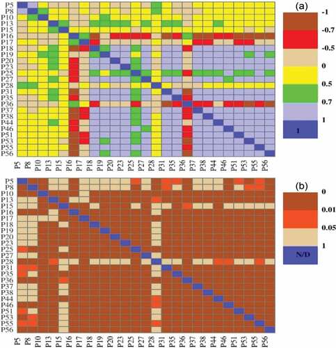
To establish the performance of the cross-correlation of piezometric influences on the reconstructed/imputed groundwater-level time series, we computed a Pearson cross-correlation matrix (Fig. 3(a)), which is further assessed by the statistical significance test (Fig. 3(b)). One can see from Fig. 3 that there are strong direct (0.7–1) and inverse (–0.5 to −1) correlations in nearly half of the piezometers, most of which range between significance levels of 0.01 and 0.05, while only a few exhibit a significance level above the predetermined value of α = 0.05 (Fig. 3(b)).

Figure 3. (a) Pearson cross-correlation matrix for all piezometric stations, with (b) significant levels. Note that N/D in the diagonals denotes that the autocorrelation significances has not been defined.

5.2 Pdf-fitting of piezometric data histograms

According to the AIC obtained by applying the nonlinear least squares approach, the most suitable pdf was identified for each piezometer (Table 2). Some of the results representing different types of pdfs are illustrated in Fig. 4.

Figure 4. Histograms for the selected piezometers representing different types of probability distribution function (pdf) (see Table 2).

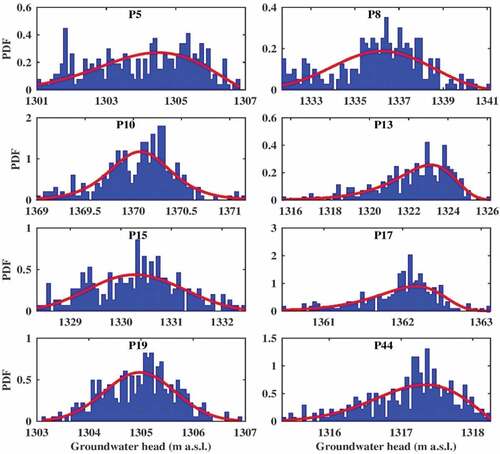
Table 2. The most suitable fitted probability distribution function, pdf (based on AIC) for each piezometer. GEV: generalized extreme value.

Piezometer	Fitted pdf	AIC
P5	GEV	998.70
P8	GEV	1107.00
P10	Logistic	258.50
P13	Extreme value	1023.00
P15	GEV	587.50
P16	Rectangular (uniform)	629.40
P17	Weibull	372.90
P18	Rectangular (uniform)	1401.00
P19	Rician	605.30
P20	GEV	1055.00
P23	GEV	941.70
P25	GEV	1564.00
P27	Rectangular (uniform)	926.00
P28	GEV	422.00
P31	Rectangular (uniform)	1814.00
P35	Rectangular (uniform)	955.30
P36	T-location-scale	1315.00
P37	Rectangular (uniform)	756.20
P38	Rectangular (uniform)	1798.00
P44	GEV	503.00
P46	GEV	1357.00
P51	Rectangular (uniform)	1984.00
P53	Rectangular (uniform)	1835.00
P55	Rectangular (uniform)	852.70
P56	Rectangular (uniform)	1431.00

From Table 2, seven types of pdfs can be discerned: generalized extreme value (GEV), logistic, extreme value, Weibull, rectangular (uniform), Rician and t-location-scale. Of these, the rectangular (uniform) and GEV distributions are found to be the most frequent pdfs, fitted to 11 and 9 piezometric stations, respectively.

As shown later, an empirical histogram that deviates more from the normal distribution has led to a poorer performance of time series decomposition. Accordingly, a poorer performance of the gap-filling procedure, applied by means of SSA and/or MSSA, has been recorded (Linnik and Ostrovskiĭ 1977), even though this is not the only controlling factor in that regard.

5.3 Identifying optimal window length for SSA and MSSA

As the most important parameters influencing the goodness-of-fit of the reconstructed groundwater levels, we identified the optimal window length (L) and the eigentriple types for each piezometer. Theoretically, the total number of observations for each piezometer is 307; however, according to Table 1 and based on the percentage of missing data for each piezometer, this value varies from 189 to 292, and the effective value of L for each piezometer was between 100 and 154 for SSA. However, the same does not hold for the window length (M) in MSSA. Indeed, it tends to be the smallest possible window length (e.g. M = 2) for most of the piezometers, because in this method there are few complete lag vectors for large values of M in the given pattern of the series (Golyandina et al. 2015).

Therefore, in an attempt to provide a more objective criterion for assigning an optimal window length in SSA, Golyandina (2010) analysed the suitability of the rule m = βN with β ≈ 0.5. Golyandina (2010) noticed that the use of a value of β close to 0.5 will yield optimal signal–noise separation and recommended that L be selected close to one-half of the time series length in most cases. However, the results obtained by Khan and Poskitt (2013) could not corroborate the findings of Golyandina (2010), whose recommendation is based primarily on simulation evidence derived from time series constructed using deterministic trigonometric signals. Khan and Poskitt (2013) found that the same procedure for estimation of the optimal window length does not apply to more general stochastic processes, where small values of L can be also optimal.

Although many applications (e.g. Kondrashov et al. 2010, Khan and Poskitt 2013, Golyandina and Korobeynikov 2014, Wang et al. 2015) have identified the optimal window length as half of the time series length, to find an optimal window length for each of the piezometric stations, we assessed a range of window lengths (approx. ±5% of half of the complete time series length N). Again the root mean square error (RMSE) was used as an objective function to identify the window lengths appropriate for imputation of missing values, as well as the complete reconstruction of groundwater-level time series using both SSA and MSSA.

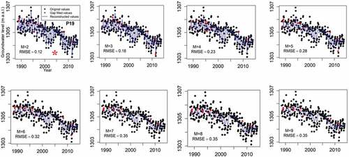
For instance, a range of window lengths was evaluated for piezometers P56 and P19 (Fig. 5), which have the highest and lowest percentage of missing values, respectively (see Table 1). Piezometer P19 contains 292 valid observations; therefore, theoretically (as recommended by several studies), the window length should be selected as L = N/2 = 146. Nevertheless, as shown for P19, the optimal window length obtained for SSA can be 137, 148 or 157, based on the computed RMSE of 0.23. However, for the imputation and reconstruction using SSA for P19, we used the window length that is closer to L = N/2, which is 148. Interestingly, the same does not hold for MSSA. As illustrated in Fig. 6, the window lengths assessed for MSSA vary from 2 to 9, while half of the time series length (N/2 = 25/2) for MSSA is about 12. Fig. 6 shows that the discrepancy, quantified via RMSE, between the observed and reconstructed time series for P19 increases monotonously from M = 2 to M = 9. Thus, we applied M = 2 to the MSSA model for imputation and reconstruction.

Figure 5. The selected window length, L (denoted by *) under SSA gap filling and reconstruction for P19 using objective function RMSE.

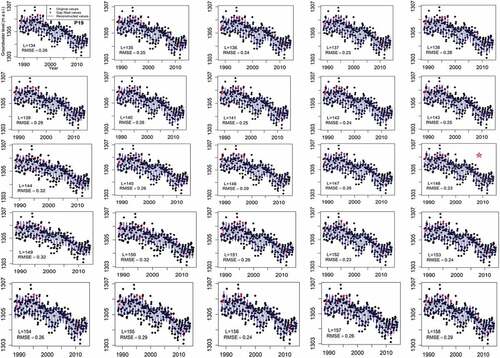
Figure 6. The selected window length, M (denoted by *) under MSSA gap filling and reconstruction for P19 using objective function RMSE.

Similarly, the same procedure was followed for piezometer P56, which contains the highest percentage of missing values (Table 1). Given the fact that the number of valid observations for P56 is 189, the number of window lengths tested fall below and above half of the time series length (i.e. N/2 = 189/2), which varies from 81 to 105 (Fig. 7). The lowest RMSE (1.11), was obtained for L = 103. Likewise, the window lengths assessed for MSSA ranged from 2 to 9. Likewise to P19, M = 2 delivered the lowest RMSE which indicates that this number is the optimal window length for MSSA (Fig. 8).

Figure 7. The selected window length, L (denoted by *) under SSA gap filling and reconstruction for P56 using objective function RMSE.

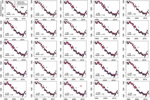
Figure 8. The selected window length, M (denoted by *) under MSSA gap filling and reconstruction for P56 using objective function RMSE.

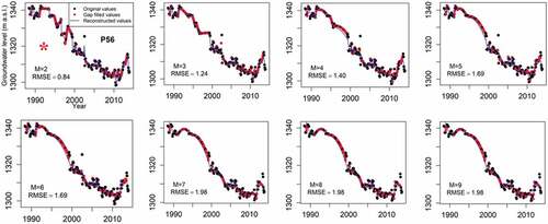
One should note that due to the fact that the valid length of observations (non-missing observations) of P19 is considerably longer than that of P56, a lower discrepancy, as quantified by RMSE of 0.23–0.32 for SSA and 0.12–0.35 for MSSA, was obtained for P19 compared with P56, where the RMSE is in the range 1.11–2.26 for SSA and 0.84–1.98 for MSSA.

Based on the above results, which show that the identified optimal window length varies around half of the time series length for SSA. In contrast, this is not the case for the MSSA, where the length of the time series is equal to the number of variables (N = 25 in this study), much smaller optimal lengths (i.e. M = 2 < N/2) are obtained. This finding is corroborated by Khan and Poskitt (2013), who showed that such small window lengths (M < N/2), can deliver a better performance of the MSSA method.

5.3.1 SSA/MSSA – reconstruction of groundwater levels

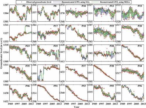
For the reconstruction of the groundwater levels, firstly, comparisons were made using a set of statistical criteria, namely R² and NS (Table 3), calculated between the observed and reconstructed groundwater levels; secondly, these results were further evaluated by graphical comparisons (see Figs. 9–11).Concerning the graphical illustration, to clearly see where the missing values exist over the time series, the original/incomplete groundwater-level time series of each piezometric station is displayed in Fig. 9.

Figure 9. Original groundwater-level time series containing missing values represented by discontinuous time series in eight selected piezometric stations.

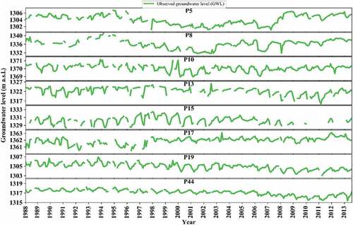
Table 3. Comparison of SSA and MSA in reconstruction of the groundwater-level time series for 25 piezometric stations.

	SSA		MSSA
Piezometer	R^2	NS	R^2	NS
P5	0.93	0.93	0.98	0.98
P8	0.83	0.83	0.97	0.97
P10	0.80	0.79	0.90	0.90
P13	0.86	0.86	0.82	0.81
P15	0.76	0.75	0.89	0.89
P16	0.92	0.90	0.93	0.92
P17	0.83	0.83	0.90	0.90
P18	0.98	0.98	0.99	0.99
P19	0.81	0.81	0.93	0.93
P20	0.97	0.97	0.98	0.98
P23	0.98	0.98	0.98	0.98
P25	0.80	0.79	0.96	0.96
P27	0.95	0.95	0.99	0.99
P28	0.77	0.77	0.90	0.90
P31	0.99	0.99	1.00	1.00
P35	0.83	0.74	0.99	0.99
P36	0.97	0.96	0.97	0.97
P37	0.98	0.98	0.99	0.99
P38	1.00	1.00	1.00	1.00
P44	0.87	0.86	0.97	0.97
P46	0.96	0.96	0.99	0.99
P51	1.00	1.00	1.00	1.00
P53	0.99	0.99	1.00	1.00
P55	0.95	0.95	0.99	0.99
P56	0.99	0.99	0.99	0.99

Based on the complete reconstruction of groundwater levels and the missing values imputed for all of the piezometric stations, overall, both SSA and MSSA could quite sufficiently reproduce the groundwater levels, as the obtained R² and NS values tend towards 1 for nearly all the piezometric stations. Meanwhile, MSSA outperformed SSA in terms of complete reconstruction of the groundwater levels, except for P13 and P36 where SSA returned a slightly better performance than MSSA (see Table 3, Figs. 10 and 11). Specifically, SSA delivered the best performance for P38 – the calculated R² and NS are 0.99 and 0.99, respectively – while we found a poor performance of SSA for P15, with R² and NS of 0.75 and 0.74, respectively.

Figure 10. Comparison of the reconstructed groundwater levels (GWL) and gap values filled using SSA and MSSA models for eight selected piezometers.

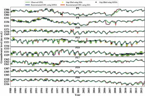
Figure 11. Reconstructed groundwater level using SSA and MSSA for 25 piezometric stations.

The same is not true for MSSA, as the best and worst matches between the observed and reconstructed groundwater levels are seen for P51 and P13, respectively. The R² and NS calculated for P51 with this approach are 0.99 and 0.99, whereas these metrics computed for P13 are 0.81 and 0.81, respectively. Since MSSA is not only reliant upon temporal correlations but also takes spatial correlations into account. In the evaluation of this method over SSA at each piezometer, this should be considered (Kondrashov and Ghil 2006, Kondrashov et al. 2010). Therefore, it can be inferred from the correlation matrix (Fig. 3(a)) that there is no strong correlation between P13 and the other piezometric stations (defined here for correlation coefficients ranging between 0.70 to 1 for direct correlation and between −0.7 and −1 for inverse correlation). Above all, in this time series for P13, the values are fitted to the extreme value distribution function (Table 2) which is only suitable for minimum values (Karian and Dudewicz 2011) and as such, the decomposition cannot be made as good as it is possible in a time series resembling a normal distribution. As mentioned earlier, the minor discrepancy found between the reconstructed and observed groundwater levels in P38 and P51 (using SSA and MSSA, respectively) demonstrates the impact of the time series’ pdf type on the quality of the reconstruction. When both R² and NS values tend to 1, that means not only that the major fraction of the observed variance is explained by the simulated/predicated data, but also that the discrepancy between the observed and simulated values is very small. This is mostly the case in the present application of SSA and MSSA to reconstruct groundwater levels. Based on the results given in Table 3 and illustrated in Figs. 10 and 11, the reconstructed groundwater levels not only closely follow (mimic) the trend of the observed groundwater levels, but also closely match (subtle discrepancy) the observed groundwater levels. Ergo, both NS and R² tend to be very close together and are, specifically, close to 1.

Moreover, our findings show that, since recharge and discharge periods have had a seasonal impact on the groundwater level, the sinusoidal eigentriples should also reasonably well reflect these oscillations in the filled gap values. Therefore, the structure and shape of the time series is very important to choose the suitable eigentriples (Supplementary material, Fig. S5). In this context, Plaut and Vautard (1994) found that a harmonic oscillation in a data series can be detected using three properties: (a) an eigen-pair (sine and cosine) of modes that explains almost identical amounts of variance; (b) the two corresponding EOF time sequences are somehow periodic and in quadrature; and (c) the associated principal component time series are in quadrature (Rangelova et al. 2012).

5.3.2 Cross-validation analysis

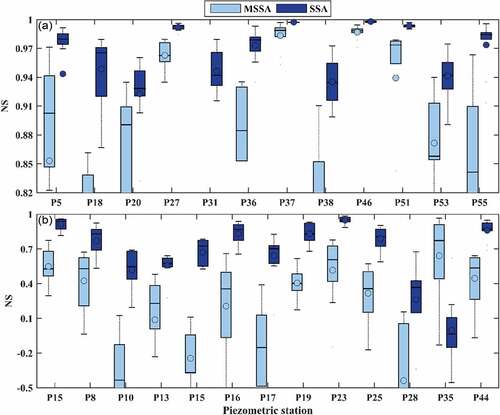
Validation of the two methodologies, i.e. SSA and MSSA, was undertaken using the k-fold cross-validation approach. As illustrated by box-and-whisker plots (Fig. 12), depending on the piezometric station, the NS calculated for the observed data (the data removed artificially) and imputed values explains a great deal of the variation. However, one can see that, for most of the piezometers, there is a narrow degree of dispersion in terms of NS (≥0.5). Nevertheless, by considering the second quartile (the band inside the boxes showing the median), most of the NS values calculated for both methods, SSA and MSSA, range above 0.5. As indicated, the observed groundwater level is reproduced quite satisfactorily for piezometric stations P37, P46, P51 (Fig. 12(a)), while a large degree of dispersion is seen for piezometers P15, P28 and P53 (Fig. 12(b)). Unlike the goodness-of-fit results obtained from the reconstructed groundwater levels for the complete time series (Table 3, Figs. 10 and 11), where MSSA shows a better performance, according to the cross-validation results, half of the piezometers (P5, P13, P15, P16, P18, P23, P27, P31, P36, P37, P44, P46 and P55) exhibit a narrower range of NS when using the SSA technique, and accordingly, a higher agreement between the observed and imputed groundwater levels; for the rest of the piezometers, MSSA is able to fill the artificial gaps with a smaller degree of error. These results are in agreement with the results of the previous analysis of the reconstruction performance of SSA and MSSA. For instance, MSSA can not produce better results for piezometers P13 and P36, similar to what has been found in the assessment part (see Table 3 and Fig. 10). Given that the best and worst performance achieved in the reconstruction procedure (Section 5.3.1) differs from those obtained in the cross-validation analysis here, the best and worst degree-of-fit using SSA are found for P37 and P35, respectively, compared with P38 and P15, respectively, in the reconstruction.

Figure 12. Box-and-whisker plots for the assessment of SSA and MSSA methods in terms of Nash-Sutcliffe efficiency (NS) for artificial gap values induced during cross-validation analysis for each piezometric station: (a) minimum and (b) maximum variability of NS in the piezometric stations.

Regarding the performance of MSSA in the validation step, we find the highest and lowest discrepancy for P37 and P28, respectively, whereas in the reconstruction step this is the case for P51 and P13, respectively. Above all, some of the artificially generated gaps adjoin to the real (existing) gaps, leading to longer missing segments in some of the piezometric stations, neither SSA or MSSA could satisfactorily impute these consecutive missing values, in comparison with the situations where the artificial gaps did not create long consecutive missing values.

6 Concluding remarks

In this paper, singular spectrum analysis (SSA) and multichannel singular spectrum analysis (MSSA) were applied to fill gaps that occurred, for different reasons, in the groundwater level values measured in 25 piezometric stations in Ardabil Plain, Iran. The results indicate that both SSA and MSSA are able to quite satisfactorily impute the missing groundwater levels, although, due to the spatial correlation observed between piezometers and the type of probability distribution function (pdf) fitted to each piezometer data series, the obtained performance differs as well. Thus, for piezometers where a strong relationship with groundwater level data at other stations is found in terms of Pearson correlation and significance, the MSSA model can better reconstruct the groundwater levels, because this method takes advantage of the spatial correlation. Also, interestingly, the type of pdf has a considerable impact on the performance of the methods. As a groundwater-level time series deviates from a normal/Gaussian distribution (e.g. extreme value distribution), a bigger discrepancy between the reconstructed and observed groundwater-level time series is detected. Conversely, we recognized a stronger agreement between the reconstructed and observed groundwater-level time series for those piezometers whose time series is closer to the normal distribution functions (e.g. uniform distribution).

In addition, our findings demonstrate that, depending on the applied method, the suitable window length can be different. Although the window lengths of the SSA tend to be around half of the length of the time series of each piezometer, this was is not the case for MSSA, where smaller window lengths could deliver a better imputation and reconstruction. Also, the appropriate eigentriples used in this study are found to be sinusoidal, which is much in accordance with the seasonal fluctuations of the groundwater level in response to recharge and discharge periods. The cross-validation analysis indicates that both methods can impute the groundwater level for artificially induced gaps very well in nearly all piezometers, even though SSA yields, overall, better results in terms of NS (≥0.7).

For future study, it is proposed to compare these two methods with other data-driven models for filling gaps in hydrological time series. Moreover, in the light of the capability of SSA and MSSA to decompose groundwater-level time series, separating the pumping effects from climatic stresses (e.g. drought events) on the groundwater-level trend and seasonality/periodicity can be of paramount importance for prospective investigations.

Acknowledgements

The authors would like to thank Regional Water Company of Ardabil, Iran for providing the groundwater-level data. Also, we would like to extend our special gratitude to Dr Hussein Akbari who greatly assisted in collecting the data used in this study.

Disclosure statement

No potential conflict of interest was reported by the authors.

Supplemental material

Supplemental data for this article can be accessed here.

Additional information

Funding

The authors are grateful to Deutscher Akademischer Austauschdienst (DAAD) for awarding a scholarship to the first author to support this project under the funding programme: Sustainable Water Management: Study Scholarships and Research Grants 14 [56322373].

References

- Adeloye, A.J., 1996. An opportunity loss model for estimating the value of streamflow data for reservoir planning. Water Resources Management, 10 (1), 45–79. doi:10.1007/BF00698811
- Adeloye, A.J., 2009. Multiple linear regression and artificial neural networks models for generalized reservoir storage-yield-reliability function for reservoir planning. Journal of Hydrologic Engineering, 14 (7), 731–738. doi:10.1061/(ASCE)HE.1943-5584.0000041
- Adeloye, A.J., Rustum, R., and Kariyama, I.D., 2011. Kohonen self-organizing map estimator for the reference crop evapotranspiration. Water Resources Research, 47. doi:10.1029/2011WR010690
- Agac, K., Baydaroglu, Ö., and Kocak, K., 2015. Reconstruction of gaps in flow series using Singular Spectrum Analysis (SSA) and Multi-channel SSA (M-SSA). In: 27th conference on weather analysis and forecasting/23rd conference on numerical weather prediction, 28 June–3 July, Chicago, IL.
- Allen, M.R. and Robertson, A.W., 1996. Distinguishing modulated oscillations from coloured noise in multivariate datasets. Climate Dynamics, 12 (11), 775–784. doi:10.1007/s003820050142
- Alley, W.M., Reilly, T.E., and Franke, O.L., 1999. Sustainability of ground-water resources. Denver, CO: US Geological Survey Circular 1186; Branch of Information Services distributor; US Department of the Interior.
- Allison, P.D., 2001. Missing data. Pennsylvania, PA: Sage Publications.
- Amer, R., et al., 2012. Groundwater quality and management in arid and semi-arid regions: case study, Central Eastern Desert of Egypt. Journal of African Earth Sciences, 69, 13–25. doi:10.1016/j.jafrearsci.2012.04.002
- Ardabil Regional Water Authority, 2013. Investigation of groundwater balance in Ardabil Plain. Ardabil: Ardabil Regional Water Authority.
- Arlot, S. and Celisse, A., 2010. A survey of cross-validation procedures for model selection. Statistics Survey, 4, 40–79. doi:10.1214/09-SS054
- Asfahani, J., 2016. Hydraulic parameters estimation by using an approach based on vertical electrical soundings (VES) in the semi-arid Khanasser valley region, Syria. Journal of African Earth Sciences, 117, 196–206. doi:10.1016/j.jafrearsci.2016.01.018
- Ball, D., 2003. Statistical analysis with missing data, 2nd edition. Journal of Marketing Research, 40 (3), 374.
- Bardossy, A. and Pegram, G., 2014. Infilling missing precipitation records – a comparison of a new copula-based method with other techniques. Journal of Hydrology, 519, 1162–1170. doi:10.1016/j.jhydrol.2014.08.025
- Bashir, F. and Wei, H.L., 2018. Handling missing data in multivariate time series using a vector autoregressive model-imputation (VAR-IM) algorithm. Neurocomputing, 276, 23–30. doi:10.1016/j.neucom.2017.03.097
- Benzvi, M. and Kesler, S., 1986. Spatial approach to estimation of missing data. Journal of Hydrology, 88 (1–2), 69–78. doi:10.1016/0022-1694(86)90197-6
- Broomhead, D.S. and King, G.P., 1986. Extracting qualitative dynamics from experimental-data. Physica D. Nonlinear Phenomena, 20 (2–3), 217–236. doi:10.1016/0167-2789(86)90031-X
- Buttlar, J.V., Zscheischler, J., and Mahecha, M.D., 2014. An extended approach for spatiotemporal gapfilling: dealing with large and systematic gaps in geoscientific datasets. Nonlinear Processes in Geophysics, 21 (1), 203–215. doi:10.5194/npg-21-203-2014
- Cheema, J.R., 2014. A review of missing data handling methods in education research. Review of Educational Research, 84 (4), 487–508. doi:10.3102/0034654314532697
- Dax, A., 1985. Completing missing groundwater observations by interpolation. Journal of Hydrology, 81 (3–4), 375–399. doi:10.1016/0022-1694(85)90039-3
- Dixon, J., 2008. Missing data: a gentle introduction. Journal of Official Statistics, 24 (2), 325–327.
- Dumedah, G. and Coulibaly, P., 2011. Evaluation of statistical methods for infilling missing values in high-resolution soil moisture data. Journal of Hydrology, 400 (1–2), 95–102. doi:10.1016/j.jhydrol.2011.01.028
- Elshorbagy, A.A., Panu, U.S., and Simonovic, S.P., 2000. Group-based estimation of missing hydrological data: II. Application to streamflows. Hydrological Sciences Journal-Journal Des Sciences Hydrologiques, 45 (6), 867–880. doi:10.1080/02626660009492389
- Enders, C.K., 2010. Applied missing data analysis. New York, NY: Guilford.
- Esmaeelzadeh, S.R., Adib, A., and Alahdin, S., 2015. Long-term streamflow forecasts by Adaptive Neuro-Fuzzy Inference System using satellite images and K-fold cross-validation (case study: Dez, Iran). Ksce Journal of Civil Engineering, 19 (7), 2298–2306. doi:10.1007/s12205-014-0105-2
- Gill, M.K., et al., 2007. Effect of missing data on performance of learning algorithms for hydrologic predictions: implications to an imputation technique. Water Resources Research, 43 (7). doi:10.1029/2006WR005298
- Golyandina, N., 2010. On the choice of parameters in singular spectrum analysis and related subspace-based methods. Statistics and Its Interface, 3 (3), 259–279. doi:10.4310/SII.2010.v3.n3.a2
- Golyandina, N., et al. 2015. Multivariate and 2D extensions of singular spectrum analysis with the rssa package. Journal of Statistical Software, 67 (2), 1–78. doi:10.18637/jss.v067.i02
- Golyandina, N. and Korobeynikov, A., 2014. Basic singular spectrum analysis and forecasting with R. Computational Statistics & Data Analysis, 71, 934–954. doi:10.1016/j.csda.2013.04.009
- Golyandina, N., Nekrutkin, V.V., and Zhigli︠a︡vskiĭ, A.A., 2001. Analysis of time series structure: SSA and related techniques. Boca Raton, FL: Chapman & Hall/CRC.
- Golyandina, N. and Zhigli︠a︡vskiĭ, A.A., 2013. Singular spectrum analysis for time series. Heidelberg: Springer.
- Gyauboakye, P. and Schultz, G.A., 1994. Filling gaps in runoff time-series in West-Africa. Hydrological Sciences Journal-Journal Des Sciences Hydrologiques, 39 (6), 621–636. doi:10.1080/02626669409492784
- Hansen, B. and Noguchi, K., 2017. Improved short-term point and interval forecasts of the daily maximum tropospheric ozone levels via singular spectrum analysis. Environmetrics, 28 (8), e2479. doi:10.1002/env.v28.8
- Harvey, C.L., Dixon, H., and Hannaford, J., 2012. An appraisal of the performance of data-infilling methods for application to daily mean river flow records in the UK. Hydrology Research, 43 (5), 618–636. doi:10.2166/nh.2012.110
- Hassani, H., Heravi, S., and Zhigljavsky, A., 2009. Forecasting European industrial production with singular spectrum analysis. International Journal of Forecasting, 25 (1), 103–118. doi:10.1016/j.ijforecast.2008.09.007
- Jellalia, D., et al., 2015. Hydro-geophysical and geochemical investigation of shallow and deep Neogene aquifer systems in Hajeb Layoun-Jilma-Ouled Asker area, Central Tunisia. Journal of African Earth Sciences, 110, 227–244. doi:10.1016/j.jafrearsci.2015.06.016
- Jolliffe, I.T., 2002. Principal component analysis. 2nd ed. New York, NY: Springer.
- Jones, M.P., 1996. Indicator and stratification methods for missing explanatory variables in multiple linear regression. Journal of the American Statistical Association, 91 (433), 222–230. doi:10.1080/01621459.1996.10476680
- Kandasamy, S., et al. 2013. A comparison of methods for smoothing and gap filling time series of remote sensing observations – application to MODIS LAI products. Biogeosciences, 10 (6), 4055–4071. doi:10.5194/bg-10-4055-2013
- Karian, Z.A. and Dudewicz, E.J., 2011. Handbook of fitting statistical distributions with R. Boca Raton, FL: CRC Press, 1 online resource (xlv, 1672 pages).
- Khalil, M., Panu, U.S., and Lennox, W.C., 2001. Groups and neural networks based streamflow data infilling procedures. Journal of Hydrology, 241 (3–4), 153–176. doi:10.1016/S0022-1694(00)00332-2
- Khan, M.A.R. and Poskitt, D.S., 2013. A note on window length selection in singular spectrum analysis. Australian & New Zealand Journal of Statistics, 55 (2), 87–108. doi:10.1111/anzs.12027
- Kim, J.W. and Pachepsky, Y.A., 2010. Reconstructing missing daily precipitation data using regression trees and artificial neural networks for SWAT streamflow simulation. Journal of Hydrology, 394 (3–4), 305–314. doi:10.1016/j.jhydrol.2010.09.005
- Kim, S.H., Yang, H.J., and Ng, K.S., 2011. Incremental expectation maximization principal component analysis for missing value imputation for coevolving EEG data. Journal of Zhejiang University-Science C – Computers & Electronics, 12 (8), 687–697. doi:10.1631/jzus.C10b0359
- Kohavi, R., 1995. A study of cross-validation and bootstrap for accuracy estimation and model selection. In: Proceedings of the 14th International Joint Conference on Artificial Intelligence – volume 2, 20–25 August, Montreal, QC. San Francisco, CA: Morgan Kaufmann Publishers Inc., 1137–1143.
- Kondrashov, D., Feliks, Y., and Ghil, M., 2005. Oscillatory modes of extended Nile River records (AD 622–1922). Geophysical Research Letters, 32 (10). doi:10.1029/2004GL022156
- Kondrashov, D. and Ghil, M., 2006. Spatio-temporal filling of missing points in geophysical data sets. Nonlinear Processes in Geophysics, 13 (2), 151–159. doi:10.5194/npg-13-151-2006
- Kondrashov, D., Shprits, Y., and Ghil, M., 2010. Gap filling of solar wind data by singular spectrum analysis. Geophysical Research Letters, 37. doi:10.1029/2010GL044138
- Kord, K. and Asghari Moghaddam, A., 2014. Spatial analysis of Ardabil plain aquifer potable groundwater using fuzzy logic. Journal of King Saud University – Science, 129 (26), 129–140. doi:10.1016/j.jksus.2013.09.004
- Krause, P., Boyle, D.P., and Bäse, F., 2005. Comparison of different efficiency criteria for hydrological model assessment. Advances in Geosciences, 5, 89–97. doi:10.5194/adgeo-5-89-2005
- Lachaal, F., et al. 2011. Characterizing a complex aquifer system using geophysics, hydrodynamics and geochemistry: a new distribution of Miocene aquifers in the Zeramdine and Mahdia-Jebeniana blocks (East-Central Tunisia). Journal of African Earth Sciences, 60 (4), 222–236. doi:10.1016/j.jafrearsci.2011.03.003
- Lachin, J.M., 2016. Fallacies of last observation carried forward analyses. Clinical Trials, 13 (2), 161–168. doi:10.1177/1740774515602688
- Linnik, I. and Ostrovskiĭ, V., 1977. Decomposition of random variables and vectors. Providence, RI: American Mathematical Society.
- Liu, S.H., et al. 2019. Missing data in marginal structural models a plasmode simulation study comparing multiple imputation and inverse probability weighting. Medical Care, 57 (3), 237–243. doi:10.1097/MLR.0000000000001063
- Liu, T.H., Wei, H.K., and Zhang, K.J., 2018. Wind power prediction with missing data using Gaussian process regression and multiple imputation. Applied Soft Computing, 71, 905–916. doi:10.1016/j.asoc.2018.07.027
- Loève, M., 1977. Probability theory. 4th ed. New York, NY: Springer-Verlag.
- McKnight, P.E., et al., 2008. Missing data: a gentle introduction by. Personnel Psychology, 61 (1), 218–221.
- Miller, D., 2011. Applied missing data analysis. Journal of Official Statistics, 27 (1), 144–145.
- Mohammadi, Z., Salimi, M., and Faghih, A., 2014. Assessment of groundwater recharge in a semi-arid groundwater system using water balance equation, southern Iran. Journal of African Earth Sciences, 95, 1–8. doi:10.1016/j.jafrearsci.2014.02.006
- Moreno, S.R. and dos Santos Coelho, L., 2018. Wind speed forecasting approach based on singular spectrum analysis and adaptive neuro fuzzy inference system. Renewable Energy. doi:10.1016/j.renene.2017.11.089
- Mwale, F.D., Adeloye, A.J., and Rustum, R., 2012. Infilling of missing rainfall and streamflow data in the Shire River basin, Malawi – a self organizing map approach. Physics and Chemistry of the Earth, 50–52, 34–43. doi:10.1016/j.pce.2012.09.006
- Myung, N.K., 2009. Singular spectrum analysis. Master’s thesis. Los Angeles, CA: University of California.
- Nkiaka, E., Nawaz, N.R., and Lovett, J.C., 2016. Using self-organizing maps to infill missing data in hydro-meteorological time series from the Logone catchment, Lake Chad basin. Environmental Monitoring and Assessment, 188, 7. doi:10.1007/s10661-016-5385-1
- Nourani, V., Alami, M.T., and Vousoughi, F.D., 2015. Wavelet-entropy data pre-processing approach for ANN-based groundwater level modeling. Journal of Hydrology, 524, 255–269. doi:10.1016/j.jhydrol.2015.02.048
- Palazzo, A. and Brozovic, N., 2014. The role of groundwater trading in spatial water management. Agricultural Water Management, 145, 50–60. doi:10.1016/j.agwat.2014.03.004
- Picard, R.R. and Cook, R.D., 1984. Cross-validation of regression-models. Journal of the American Statistical Association, 79 (387), 575–583. doi:10.1080/01621459.1984.10478083
- Plaut, G. and Vautard, R., 1994. Spells of low-frequency oscillations and weather regimes in the Northern-Hemisphere. Journal of the Atmospheric Sciences, 51 (2), 210–236. doi:10.1175/1520-0469(1994)051<0210:SOLFOA>2.0.CO;2
- Rangelova, E., Sideris, M.G., and Kim, J.W., 2012. On the capabilities of the multi-channel singular spectrum method for extracting the main periodic and non-periodic variability from weekly GRACE data. Journal of Geodynamics, 54, 64–78. doi:10.1016/j.jog.2011.10.006
- Rekapalli, R., et al., 2017. 3D seismic data de-noising and reconstruction using multichannel time slice singular spectrum analysis. Journal of Applied Geophysics, 140, 145–153. doi:10.1016/j.jappgeo.2017.04.001
- Rodrigues, P.C. and de Carvalho, M., 2013. Spectral modeling of time series with missing data. Applied Mathematical Modelling, 37 (7), 4676–4684. doi:10.1016/j.apm.2012.09.040
- Schoellhamer, D.H., 2001. Singular spectrum analysis for time series with missing data. Geophysical Research Letters, 28 (16), 3187–3190. doi:10.1029/2000GL012698
- Shen, Y., Peng, F., and Li, B., 2015. Improved singular spectrum analysis for time series with missing data. Nonlinear Processes in Geophysics, 22 (4), 371–376. doi:10.5194/npg-22-371-2015
- Srebotnjak, T., et al., 2012. A global water quality index and hot-deck imputation of missing data. Ecological Indicators, 17, 108–119. doi:10.1016/j.ecolind.2011.04.023
- Statistical Center of Iran, 2011. Implementation of the 2011 Iranian Population and Housing Census. Tehran: Statistical Center of Iran.
- Symonds, M.R.E. and Moussalli, A., 2011. A brief guide to model selection, multimodel inference and model averaging in behavioural ecology using Akaike’s information criterion. Behavioral Ecology and Sociobiology, 65 (1), 13–21. doi:10.1007/s00265-010-1037-6
- Taie Semiromi, M. and Ghasemian, D., 2018. Reconstruction of water infiltration rate reducibility in response to suspended solid characteristics using singular spectrum analysis: an application to the Caspian Sea Coast of Nur, Iran. Hydrology, 5 (4), 59. doi:10.3390/hydrology5040059
- Teegavarapu, R.S.V. and Chandramouli, V., 2005. Improved weighting methods, deterministic and stochastic data-driven models for estimation of missing precipitation records. Journal of Hydrology, 312 (1–4), 191–206. doi:10.1016/j.jhydrol.2005.02.015
- Teegavarapu, R.S.V., Tufail, M., and Ormsbee, L., 2009. Optimal functional forms for estimation of missing precipitation data. Journal of Hydrology, 374 (1–2), 106–115. doi:10.1016/j.jhydrol.2009.06.014
- Thomas, B.F. and Famiglietti, J.S., 2015. Sustainable groundwater management in the arid Southwestern US: Coachella Valley, California. Water Resources Management, 29 (12), 4411–4426. doi:10.1007/s11269-015-1067-y
- Vautard, R. and Ghil, M., 1989. Singular spectrum analysis in nonlinear dynamics, with applications to paleoclimatic time-series. Physica D. Nonlinear Phenomena, 35 (3), 395–424. doi:10.1016/0167-2789(89)90077-8
- Vousoughi, F.D., et al. 2013. Trend analysis of groundwater using non-parametric methods (case study: Ardabil plain). Stochastic Environmental Research and Risk Assessment, 27 (2), 547–559. doi:10.1007/s00477-012-0599-4
- Walczak, B. and Massart, D.L., 2001. Dealing with missing data: part I. Chemometrics and Intelligent Laboratory Systems, 58 (1), 15–27. doi:10.1016/S0169-7439(01)00131-9
- Walker, D., et al., 2016. Filling the observational void: scientific value and quantitative validation of hydrometeorological data from a community-based monitoring programme. Journal of Hydrology, 538, 713–725. doi:10.1016/j.jhydrol.2016.04.062
- Wang, R., et al. 2015. Selection of window length for singular spectrum analysis. Journal of the Franklin Institute, 352 (4), 1541–1560. doi:10.1016/j.jfranklin.2015.01.011
- World Meteorological Organization, 2008. Manual on low-flow estimation and prediction. Geneva: World Meteorological Organization.
- Wosten, J.H.M., Pachepsky, Y.A., and Rawls, W.J., 2001. Pedotransfer functions: bridging the gap between available basic soil data and missing soil hydraulic characteristics. Journal of Hydrology, 251 (3–4), 123–150. doi:10.1016/S0022-1694(01)00464-4
- Wu, X., et al., 2016. Optimizing conjunctive use of surface water and groundwater for irrigation to address human-nature water conflicts: a surrogate modeling approach. Agricultural Water Management, 163, 380–392. doi:10.1016/j.agwat.2015.08.022
- Zaidi, F.K., et al., 2015. Identification of potential artificial groundwater recharge zones in Northwestern Saudi Arabia using GIS and Boolean logic. Journal of African Earth Sciences, 111, 156–169. doi:10.1016/j.jafrearsci.2015.07.008
- Zhang, Z.H., 2016. Missing data imputation: focusing on single imputation. Annals of Translational Medicine, 4 (1). doi:10.21037/atm.2016.04.05
- Zhou, Y., et al. 2013. Upgrading a regional groundwater level monitoring network for Beijing Plain, China. Geoscience Frontiers, 4 (1), 127–138. doi:10.1016/j.gsf.2012.03.008
- Zotov, L., et al. 2017. Multichannel singular spectrum analysis of the axial atmospheric angular momentum. Geodesy and Geodynamics, 8 (6), 433–442. doi:10.1016/j.geog.2017.02.010