Comparing 2D capabilities of HEC-RAS and LISFLOOD-FP on complex topography

ABSTRACT

This study evaluates and compares two-dimensional (2D) numerical models of different complexities by testing them on a floodplain inundation event that occurred on the Secchia River (Italy). We test 2D capabilities of LISFLOOD-FP and HEC-RAS (5.0.3), implemented using various grid sizes (25–100 m) based on 1-m DEM resolution. As expected, the best results were shown by the higher-resolution grids (25 m) for both models, which is justified by the complex terrain of the area. However, the coarser resolution simulations (50 and 100 m) performed virtually identically compared to the high-resolution simulations. Nevertheless, the spatial distribution of flood characteristics varies: the 50 and 100 m results of LISFLOOD-FP and HEC-RAS misestimated flood extent and water depth in selected control areas (built-up zones). We suggest that the specific terrain of the area can cause ambiguities in large-scale modelling, while providing plausible results in terms of the overall model performance.

KEYWORDS:

• floodplain inundation
• hydraulic modelling
• two-dimensional models
• DEM resolution

Editor A. Fiori Associate editor E. Volpi

1 Introduction

Recent and historical data demonstrate the large share of monetary damage and fatalities that can be attributed to hydrological natural hazards (Munich Re 2015). Some of the most costly floods in the past decades occurred in central European countries; for example, the 2002 flood resulted in US$16.5 billion damages and that in 2013 about US$12.5 billion damages, and together they caused 64 deaths (Munich Re 2015). Additionally, a related issue is climate change, which will likely affect the frequency and magnitude of floods in the future (Milly et al. 2002, Lehner et al. 2006, Alfieri et al. 2015, Arnell and Gosling 2016). With global economic and population growth, the consequences of severe flooding events induced by climate change are likely to increase in the future, so the overall flood risk is projected to increase significantly (Alfieri et al. 2017). Although some studies demonstrate the difficulty of predicting future flood frequency and magnitude changes due to the high complexity of forcing mechanisms, it is evident that the flood damages will continue to grow (Kundzewicz et al. 2013). Such conditions emphasise the importance of developing efficient flood-risk management strategies which would help to lower the upcoming losses. The 2007 European Flood Directive (2007/60/EC), among others, contributes to increasing resilience to hydrological natural disasters by requiring each EU Member States to develop cyclically updated flood hazard and risk maps and establish long-term management plans (EC 2007).

The Flood Directive identifies flood risk as “a product of the probability of the flood event and its potential adverse consequences” (EC 2007), and it has to be re-assessed and updated every six years. Therefore, a crucial element in flood-risk assessment is efficient and accurate flood hazard mapping and, functional to this, the identification of the most suitable models and tools for adequately addressing this task, thereby enhancing the overall quality of risk analysis.

A considerable number of studies have demonstrated the use of the one- and two-dimensional (1D and 2D) numerical models to delineate floodplains (Bates and de Roo 2000, Aronica et al. 2002, Horritt and Bates 2002, Büchele et al. 2006, de Moel et al. 2009, Di Baldassare et al. 2009, 2010, Neal et al. 2012, Falter et al. 2013, Domeneghetti et al. 2013, 2015, Alfieri et al. 2014), which allow an accurate representation of river hydraulics and floodplain inundation dynamics. There is an ongoing debate, however, on which schematization under which conditions should be used (1D, coupled 1D/2D or fully 2D) (Apel et al. 2009).

Recent studies suggest using fully 2D models with high levels of detail in order to avoid uncertainties and limitations coming from the incorrect interpretation of flood dynamics and unrealistic reproductions of the terrain topography (Morsy et al. 2018). Some studies, however, point out that for the large-scale studies, coarser resolution (i.e. 50 m) is an optimum between the accuracy and computational expenses for 2D simulations (Savage et al. 2016). While 1D models have proved to be able to represent the processes within the channel, the flood wave dynamics across inundated floodplains can be only captured using 2D scheme (Tayefi et al. 2007, Falter et al. 2013). Using fully 2D codes can, however, be difficult, as most areas are not covered by the high-resolution terrain datasets (LiDAR surveys) that such modelling requires. In addition, another evident constraint of using fully 2D codes lies in their higher computational burden relative to simplified coupled 1D/2D codes (Apel et al. 2009, Falter et al. 2013, Dimitriadis et al. 2016). Yet, the tendency to run high-resolution global and regional flood scenarios is increasing (Falter et al. 2013, Sampson et al. 2015, Savage et al. 2016, Schumann et al. 2016). Furthermore, with increasing computational capacity, parallelization techniques and affordable access to cloud computing services, the utilization of 2D codes in combination with high-resolution DEMs becomes more and more viable for hydraulic engineers and researchers (Morsy et al. 2018). Moreover, the 20× and 100× speed-ups gained by executing codes on graphical processing units (GPU) hardware comparing to central processing unit (CPU) clusters show the potential in applying high-resolution flood models over large areas (Vacondio et al. 2014, Morsy et al. 2018).

Among 2D models, there are codes, which use fully 2D shallow-water or diffusion wave equations and those, which simplify certain terms (Teng et al. 2017). The main differences in the performance of such models lie in the governing equations used, the mesh representation (structured, unstructured, raster-based, flexible) and numerical scheme (finite-element, finite-volume, finite-difference). Simplified 2D models have a solid advantage by being computationally significantly more efficient than, for instance, fully 2D models based on the complete St Venant equation (Néelz and Pender 2013). Previous research done in this domain has covered benchmark analysis of a number of 2D codes. A benchmark study performed by the UK Environment Agency on 2D hydraulic modelling packages revealed that 2D models based on shallow-water equations deliver better results in terms of floodwater velocity, than the ones which used simplified equations (Néelz and Pender 2013). Nevertheless, the same study clearly indicates that for the representation of flood extent all 2D packages perform comparably (those which solve full shallow water equations and those, which neglect/simplify certain terms). Another benchmarking study for 2D codes was performed by Hunter et al. (2008) who compared six 2D codes of different complexity for urban flood modelling using hyper-resolution LiDAR data. They concluded that such data are accurate enough to simulate flow in urban environments, however the uncertainties arise from parameterization of the models (Hunter et al. 2008). Haile and Rientjes (2005) also investigated 2D flood modelling using LiDAR data and confirmed that urban areas require high-resolution data (maximum 15 m grid size) and additional pre-processing to represent buildings. However, such studies are applied solely for urban areas; in different landscapes (natural and artificial) the data resolution and parameterization should be further investigated.

Building on the existing literature, our study aims at further deepening our knowledge and understanding of the potential and capabilities of different types of 2D inundation models in the context of flood hazard assessment and mapping. In particular, our study compares two models, the well-known LISFLOOD-FP (Horritt and Bates 2002) and the recently launched 2D version (release 5.0.3) of Hydrologic Engineering Center-River Analysis System (HEC-RAS) model. The two codes represent different model complexities, LISFLOOD-FP is a raster-based 2D model based on inertial formulation of the shallow-water equations, while HEC-RAS is a widespread modelling tool for hydraulic engineers that can be used for a large spectrum of applications and deploy different schematization complexities, and, in more recent releases, solves the fully 2D equations.

A previous study performed by Horritt and Bates (2002) looked into differences in terms of flood extent for a 2D diffusion-wave LISFLOOD-FP model, a 1D HEC-RAS model and a 2D finite-element TELEMAC 2D model. They identified that HEC-RAS and TELEMAC 2D are different from LISFLOOD-FP because of their different response to friction coefficients used in calibration (Horritt and Bates 2002). It is important to point out, that this study is based on the older version of the models. For instance, HEC-RAS has been improved and is now used not only for 1D but also for fully 2D simulations with additional advantages of implying fully momentum shallow water equation on high-resolution DEMs with unstructured grid., LISFLOOD-FP has also been updated from a diffusion wave to inertial formulation of the shallow water equation and now uses an adaptive time step, which ensures numerical stability of the code.

The LISFLOOD-FP and HEC-RAS codes are governed not only by different schemes, but by mesh representations, capabilities and input data requirements and, hence, a thorough comparison is needed to better understand their advantages and limitations relative to topographical complexity, inundation dynamics and data availability of the codes updated versions. Regional and continental applications of LISFLOOD-FP are already a reality (Alfieri et al. 2014, Sampson et al. 2015, Schumann et al. 2016), while such applications can be envisaged in the near future for fully 2D HEC-RAS due to the rapid expansion of computational means and strategies cited above. For instance, a recent study by Liu et al. (2019) compared the 1D and 2D modules of HEC-RAS and LISFLOOD-FP where the channel flow is linked to the floodplain by lateral structures using a uniform grid resolution of 30 m. They concluded that the 2D models showed slightly better results than 1D. It is crucial to remember, that small and big changes made to the codes together with emerging accuracy of LiDAR data may drastically affect models’ performance and results. Therefore, in this study, we would focus on the newest versions of the codes and investigate the advantages disadvantages and their correlation with the DEM resolution for floodplain modelling.

Our study aims to quantitatively highlight differences and similarities in terms of accuracy of representation of inundation processes within heterogeneous floodplains and computational efficiency between the models with regard to different grid and terrain resolutions. We focused our study on such aspects as the capabilities and accuracy of 2D models of different complexity to capture flood extent and water depth in areas with complex topography. Additionally, we discuss model limitations in the context of future large-scale applications of detailed fully 2D models.

2 Tools and study scope

2.1 HEC-RAS (5.0.3)

The HEC-RAS (5.0.3) model was developed to perform fully 2D computations and solves both the 2D St Venant equations and the 2D diffusion wave equations through an implicit finite-volume solution. The selection of the equation depends on the study case (dam breach, wave propagation analysis, existence of multiple hydraulic structures within the area) (Brunner 2016). Previous studies done on benchmarking of the codes with different physical complexity showed that, in cases where subcritical flow is unlikely (gradually varied flow), simpler codes perform comparably well in terms of water depth and velocity (Neal et al. 2012, de Almeida and Bates 2013). In order to utilize more stable numerical solutions and reduce the computation time for the current case, we selected the 2D diffusion wave solver. It identifies the barotropic and bottom friction terms as prevailing.

(1) $\frac{n^2\left|V\right|V}{{\left(R\left(H\right)\right)}^{4/3}}=-\mathrm{\nabla }H$(1)

The above equation can be further rearranged by dividing both sides by the square root of their norm:

(2) $\mathit{V}=\frac{-{\left(R\left(H\right)\right)}^{2/3}}{n}\frac{\mathrm{\nabla }H}{{\left|\mathrm{\nabla }H\right|}^{1/2}}$(2)

where V is the velocity vector, R is the hydraulic radius, ∇H is the surface elevation gradient and n is Manning´s n.

The differential form of the diffusion wave approximation of the shallow water equation can be obtained by combining the diffusion wave equation in the mass conservation equation:

(3) $\frac{\mathrm{\partial }H}{\mathrm{\partial }t}-\mathrm{\nabla }\bullet \beta \mathrm{\nabla }H+q=0$(3)

where (Brunner 2016):

(4) $\beta =\frac{{\left(R\left(H\right)\right)}^{5/3}}{n{\left|\mathrm{\nabla }H\right|}^{1/2}}$(4)

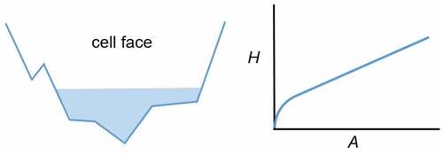
Mesh computation is done automatically within the 2D flow areas and meshes can be structured (i.e. regular connectivity) or unstructured (irregular connectivity). The selection of the grid type (structured/unstructured) depends on the terrain topography and data availability, enabling the user to adopt reduced mesh resolution in more homogenous areas and a highly detailed description along critical terrain features such as embankments or levees. Additionally, the model gives an opportunity to reduce the computation time by implementing a coarser grid on fine topographic details through a so-called sub-grid bathymetry approach (see Fig. 1) (Brunner 2016). For instance, the DEM resolution might be 2 m, while the mesh cell size is 25 m (see Fig. 1). During a pre-processing step, hydraulic radius, volume and cross-sectional data are collected for each mesh cell using the finer resolution data and stored in property tables (a function for cell-face area (A) and water surface elevation (H); see Fig. 2). The sub-grid approach allows the computation of more detailed property tables for larger mesh cell sizes.

Figure 1. RasMapper representation of 2-m sub-grid DEM and 25-m mesh cell size of HEC-RAS 2D

(adapted from Brunner 2016).

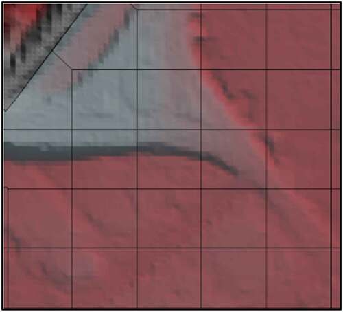
Figure 2. Cell face terrain data (left) and schematic representation of A – H (area–elevation) relationship reproduced with the property table (right)

(adapted from Brunner 2016).

2.2 LISFLOOD-FP

The LISFLOOD-FP model is a raster-based low-complexity hydraulic model, which was designed for research purposes and in particular, allows for high-resolution simulations. The model used in this paper is employed in 2D mode and solves an inertial formulation of the shallow-water equations in explicit form through a finite difference scheme (Bates et al. 2010, Savage et al. 2016). The model further simplifies the computation by decoupling flows in the x and y directions and treating the 2D problem as a series of 1D calculations through the cell face boundaries. Therefore, the water flow through each cell face is calculated as:

(5) $q_t+\mathrm{\Delta }t=\frac{q_t-g{h}_t\mathrm{\Delta }t\frac{\mathrm{\Delta }\left(h_t+z\right)}{\mathrm{\Delta }x}}{\left(1+g{h}_t\mathrm{\Delta }t{n}^2{q}_t/h_t^{10/3}\right)}$(5)

where $q_{t+\mathrm{\Delta }t}$ is a unit flow at the next time step t, g is gravitational acceleration, h is depth, n is a Manning’s roughness coefficient, Δ is the cell resolution, z is cell elevation, and $h_t$ is the difference between highest bed elevation and highest water surface elevation between two cells (Bates et al. 2010, Savage et al. 2016).

The discharge through the four faces of each cell is then used to update the water depth in each cell at each time step:

(6) $\frac{\mathrm{\Delta }{h}^{ij}}{\mathrm{\Delta }t}=\frac{Q_x^{i-1,j}-Q_x^{i,j}+Q_y^{ij-1}-Q_y^{i,j}}{\mathrm{\Delta }{x}^2}$(6)

where i and j are the coordinates of a cell (Coulthard et al. 2013).

In order to secure the model stability we used an adaptive time step based on the Courant-Friedrichs-Lewy (CFL) condition which is estimated as (Bates et al. 2010):

(7) $\mathrm{\Delta }{t}_{\mathrm{m}\mathrm{a}\mathrm{x}}=\alpha \frac{\mathrm{\Delta }x}{\sqrt{g{h}_t}}$(7)

where$\alpha$ is a coefficient ranging from 0.3 to 0.7, which ensures the numerical stability (Coulthard et al. 2013).

Despite the governing equations used to compute the flow between cells, another important distinction between the two models is the way in which the codes treat topographic data. Differently from HEC-RAS, mesh size in LISFLOOD-FP is forced by the resolution of the input DEM data and cannot be further manipulated. There is not an option to include sub-grid (see details above) terrain in the 2D computations with larger mesh sizes, meaning the mesh face cross-section profile has a rectangular shape.

2.3 Objective of the study

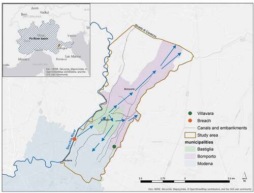
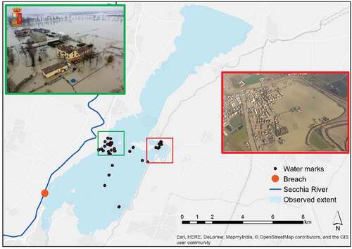
Our study tests and compares the models on an inundation event that occurred on 19 January 2014 in the dike-protected floodplain of the Secchia River (a right bank tributary of the Po River), in northern Italy (Fig. 3). We compare HEC-RAS with LISFLOOD-FP using various grid sizes of 25, 50 and 100 m, generated from a LiDAR DEM of 1-m resolution. Moreover, along with the resampled DEMs, we use the sub-grid capabilities of HEC-RAS by applying sub-grid terrain of 1-m resolution within the 25-, 50- and 100-m sized meshes.

Figure 3. Breach location and flow direction during the event.

We explicitly focus on the fully 2D formulations for both models addressing the representation of the floodplain wave dynamics, i.e. no 1D component is included in the simulations (no channel flow simulated). This is done in order to see the difference in the codes’ ability to simulate inundation propagating over complex topography and an initially dry floodplain.

3 Study event and data used, model set-up and calibration

3.1 Study event and data

The event was characterized by a levee breach and consequent flooding of over 50 km² of the plain behind the dike within 48 h causing significant population displacement, one death and economic losses in excess of 400 million Euro (D’Alpaos et al. 2014, Carisi et al. 2018). It occurred around 06:00 h on 19 January when a part of the levee in the right bank of the Secchia River collapsed (Fig. 3). Although the water levels in the river did not exceed the designed embankment crest height, right after the breach the crest lowered by about 1 m compared to the water elevation in the Secchia River. The conclusion derived from the post-event analysis is that the reason for the levee collapse was the activity of burrowing animals in the area (Orlandini et al. 2015, Vacondio et al. 2016).

During the event the breach width reached nearly 100 m and the inflow water volume that penetrated the floodplain reaching the municipalities of Modena, Bastiglia and Bomporto was estimated in 38.7 × 10⁶ m³ (Fig. 4). Previous studies showed that linear terrain irregularities strongly affected the flooding dynamics (Castellarin et al. 2014, Domeneghetti et al. 2014, Hailemariam et al. 2014, Carisi et al. 2018). Post-event field surveys made by the local authorities together with other publicly available data (photographs, videos and Google Earth^TM images) provided us with the watermarks (maximum water depths) at certain points. The study of Horritt et al. (2010) shows that the post-event collection and evaluation of the watermarks and wreck marks does not always match the actual maximum values. Field measurement methods and their interpretation done by surveying groups, approximations of the elevation of watermarks acquired from images may produce uncertainties. Horritt et al. (2010) report that accuracy range in such estimations is likely to be up to 0.5 m, which could be a potential source of errors. In order to check the liability of the observed watermarks, we plotted them in relation to the 1-m LiDAR DEM to see if there are water surface elevation outliers (points in closer vicinity to the large difference in depth). We looked at their weighted average and observation difference and removed the outliers (>0.5 m). As a result, we further used 46 watermark points to validate the maximum simulated water depth. However, we left the points at very close distances from each other (<50 m) to look at the model performance with different sub-grid configurations.

Figure 4. Outflowing discharge at the levee breach point over time

(adapted from D’Alpaos et al. 2014).

Official reports recorded vast damage in the small town of Bomporto (Carisi et al. 2018). During the event, the area within the embankment was completely flooded (Fig. 5). We selected the area surrounding this particular town due to its complex and highly anthropogenically altered terrain (e.g. minor levees, embankments, irrigation and drainage channel networks, etc.) to test how the models were able to reproduce the propagation of inundated extent in such topography. The watermarks are located within the populated areas; therefore they are concentrated within the affected settlements of Bastiglia and Bomporto and the close vicinity around them. Fewtrell et al. (2008) in their study explicitly showed that the 2D models' behaviour is strongly affected by the heterogeneity of the urban fabric and requires a very fine mesh to represent the building dimensions. Thus, we are particularly interested in how the selected models will perform in built-up zones. We used these data to validate the models by comparing them to maximum water depths observed during the event (Carisi et al. 2018). The study by Carisi et al. (2018) reproduced the Secchia event simulating the inundation dynamic. The simulations of Carisi et al. (2018) were based on the higher resolution 1-m LiDAR DEM with unstructured mesh, whose faces ranged in size from 1 to 200 m in more homogenous zones. The linear terrain irregularities were explicitly represented. The official reports done on the post-event field data collection and simulations made possible to reconstruct the flood extent as detailed as possible (D’Alpaos et al. 2014). The simulations showed a high correspondence with the maximum flood extent records (up to 0.9 in terms of measure of fit) (Carisi et al. 2018).

Figure 5. Observed flood extent, hotspot focus areas (green and red boxes) and watermarks (control points). The green box (top left) captures the inundation in Bastiglia; the red box (right) shows the inundation extent in Bomporto.

3.2 Model configuration and set-up

Previous modelling studies of the January 2014 inundation event showed that the topography of the area strongly controls the model performance (Vacondio et al. 2016, Carisi et al. 2018).

As our interest is to show how the models behave at large scales, we considered downscaling the 1-m LIDAR DEM to 25, 50 and 100 m by taking the mean of the pixels’ value. The vertical accuracy of the bare earth DEM is ±0.15 m (Geoportale Nazionale 2017). The study of Savage et al. (2016) on regional flood modelling showed that resolution coarser than 100 m decreases the reliability of the model outcomes; therefore, we avoided using lower resolutions. The same study showed that probabilistic flood mapping does not benefit much from resolution higher than 50 m. Nevertheless, as our study is specifically focused on heterogeneous topography, we intentionally included a 25-m DEM in order to have a more profound comparison of the two different models.

The flow leaving the breach was estimated based on the difference between observed discharge hydrographs 200 m upstream and 200 m downstream along the reach (see Fig. 4) (Vacondio et al. 2016).

Both models were constructed adopting the same hydraulic loads. The upstream boundary condition was represented by the discharge flowing through the levee breach and it was fixed in each simulation as a point (a pixel) located at the failure location. The breach width was set in all simulations equal to 100 m, simultaneously involving 1, 2 and 4 pixels in the simulations using 100-, 50- and 25-m resolutions, in this order. The inflow hydrograph was represented by the values retrieved from the studies of Carisi et al. (2018), Vacondio et al. (2016) and Orlandini et al. (2015). In order to avoid possible errors coming from different widths of the upstream boundary (levee breach breadth), we insured that the watermarks are located further downstream from the inflow location.

We referred to the CORINE Land Cover (EEA 2007) and OpenStreetMap (Contributors OSM 2012) datasets for classifying land-use in the study area, which we represented in the models using spatially varying roughness coefficients. In particular, we adopted a subdivision of the study area into two main classes: built-up (i.e. urban and industrial zones) and rural (i.e. all other land-use types mostly represented as agricultural fields) areas.

The fully 2D HEC-RAS model was used and tested with and without its sub-grid function capability with structured mesh cell sizes of 25 × 25, 50 × 50 and 100 × 100 m based on the 1-m LiDAR DEM. Structured mesh selection significantly decreases the model set-up time and does not require additional data (i.e. linear infrastructure outlines) as is the case for configuration of an unstructured mesh. This is of a high importance for large-scale simulations, where such details might be unavailable, or their implementation would require significant effort.

The meshes were also used with the corresponding aggregated DEM (25 × 25 mesh with 25-m DEM resolution, 50 × 50 mesh with 50-m DEM resolution, 100 × 100 mesh with 100-m DEM resolution). Overall, we apply nine mesh/terrain configurations, as indicated in Table 1.

Table 1. Simulation configurations.

Mesh resolution	LISFLOOD	HEC RAS
		1-m sub-grid terrain resolution	25-, 50- and 100-m sub-grid terrain resolution
25	L25	HR25_1	HR25_25
50	L50	HR50_1	HR50_50
100	L100	HR100_1	HR100_100

3.3 Model calibration

The models were calibrated using roughness coefficients for HEC-RAS and LISFLOOD-FP at 25-m resolution. We looked into previous research and post-event surveys done to describe and analyse this event. In particular, we considered the publication of Carisi et al. (2018) and the accurate reconstruction of the flood extent reported therein. We compared the maximum flood extent resulting from the models with the reference flood extent from Carisi et al. (2018) by means of a well-known method to compare binary maps (wet and dry areas) of the simulated and observed extents using a performance measure (Schumann et al. 2009):

(8) $F=\frac{\mathrm{A}}{\mathrm{A}+\mathrm{B}+\mathrm{C}}\ast 100$(8)

where A is the area correctly predicted as flooded (wet in both observed and simulated), B is the area overpredicting the extent (dry in observed but wet in simulated) and C is the underpredicted flood area (wet in observed but dry in simulated). The parameter F defined in Equation (8) varies between 0% and 100%, where 100% corresponds to a perfect match between the modelled extent and the reference inundation map (Horritt and Bates 2002).

Calibration consisted of varying the Manning’s roughness coefficient, n, of rural areas from 0.03 to 0.2 by 0.005 m^−1/3 s increments, while keeping n of urbanized zones constant – 0.3 m^−1/3 s (Syme 2008) – and referring to the land-use description from CORINE Land Cover data (EEA 2007) and OpenStreetMap (2012). So, for each simulation, we would use one roughness coefficient for rural and one for urban areas. LISFLOOD-FP resulted in the highest F value (81%) for a floodplain roughness coefficient n = 0.155 m^−1/3 s; with F varying between 73% for n = 0.030 m^−1/3 s and 77% for n = 0.200 m^−1/3 s. HEC-RAS showed similar performance, with a maximum F value equal to 78% at n = 0.195 m^−1/3 s; however F values plateau at 78% for n values larger than 0.18 m^−1/3 s. For the further analysis, we selected the value of 0.195 m^−1/3 s. These values (0.195 m^−1/3 s for rural and 0.3 m^−1/3 s for urban areas) do not reflect the actual vegetation/soil cover in the area, they are aimed at compensating for the possible errors coming from the overall flooding extent used to calibrate the model and possible limitations related to the inability of the terrain to capture the linear features, which played a crucial role in routing the flow. Also, we calibrated both models at 50- and 100-m resolution, obtaining optimal values of the calibration parameters that differed from the optimal values at 25-m resolution by less than 1%. Therefore, we decided to use uniform optimal values for all resolutions.

Both models were validated against 46 watermarks (see e.g. Fig. 5) for which the maximum water depth (m) was surveyed in the event aftermath (watermarks, post-event surveys, interviews and geolocating the marks using aerial and ground photographs). Dry-simulated points were given zero value. Comparison was performed by means of Root Mean Square Error (RMSE). All simulations were performed on the four cores with the Intel Core i7 3.60 GHz CPU, 64 GB RAM.

4 Results

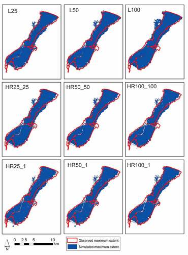
From Fig. 6, we can see that the overall performance in terms of inundation extent (i.e. F values defined as in Equation (8)) of LISFLOOD-FP is slightly better than that of HEC-RAS. The 25-m LISFLOOD-FP simulation (L25) was able to correctly simulate 81% of the flooding extent, while the 50-m LISFLOOD-FP simulation (L50) was as good as the HEC-RAS simulation with 1-m sub-grid terrain (78%). All other configurations produced almost identical results, with an F value of approx. 77%. However, the spatial pattern of the flooded areas differs for all configurations (Fig. 6).

Figure 6. Overall simulated extent for all configurations (solid blue), compared to the observed extent (red outline).

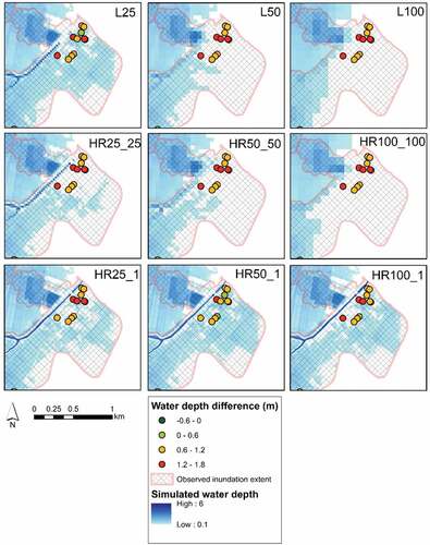
Together with the analysis of the overall inundation extent, the performance of each model was scrupulously assessed relative to specific areas in the towns of Bomporto and Bastiglia. Figure 5 illustrates the observed extent and the location of focus areas. From Fig. 7 we can see that the LISFLOOD-FP model was able to correctly simulate the maximum flood extent in Bomporto for the fine resolution of 25 m, while with other LISFLOOD-FP resolutions the same results were not achieved. The red line in these maps demarcates the observed inundation extent, so we can see that the L25 configuration output is in good agreement with the observations (the flood propagated to the observed inundation boundary and covered all watermarks). The LISFLOOD-FP 50- and 100-m simulations (L50 and L100) did not properly simulate the flood propagation in this area. The watermarks display the accuracy of predicted water levels in relation to the observations. Figure 7 shows that the flood extent simulated by HEC-RAS for 25-, 50- and 100-m mesh sizes with 1-m sub-grid terrain was consistent with the observations, especially the larger meshes of 50 and 100 m. The HEC-RAS models without sub-grid terrain (HR25_25, HR50_50 and HR100_100) were unable to simulate the flood wave propagation in the Bomporto focus area.

Figure 7. LISFLOOD-FP and HEC-RAS flood extent for different configurations at Bomporto (red box in Fig. 5). Water depth difference (m) between predicted and observed at watermark points.

As for the other focus area, from Fig. 8, we can see that the flood extent in Bastiglia produced by all LISFLOOD-FP resolutions is in line with the observed flood extent. The L25 configuration was more successful in reproducing the flood extent over the control areas, while the L50 and L100 models just slightly underestimate the flood boundaries (see Figs. 7 and 8). The HEC-RAS coarser grid simulations (25-, 50- and 100-m sub-grid), similar to LISFLOOD-FP (50- and 100-m), produce plausible results in terms of the inundation extent. The accuracy decreases with increasing mesh size. The HEC-RAS configurations using sub-grid terrain of 1 m resolution struggle to produce a continuous inundation pattern, resulting in numerous dry islands.

Figure 8. LISFLOOD-FP and HEC-RAS flood extent for different configurations at Bastiglia (green box in Fig. 5). Water depth difference (m) between predicted and observed at watermarks.

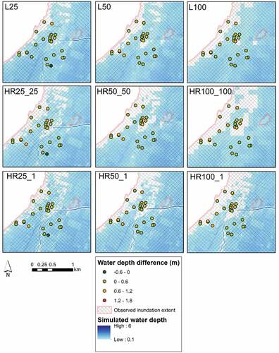
Figures 7 and 8 display the watermarks and the colour indicates on the level of absolute difference between simulated and surveyed maximum water levels through a red (underestimation) to dark green (overestimation) colour scale. The largest difference is especially visible in Bomporto focus area (up to 1.8 m), as most of the simulations did not succeed in inundating the town., while in Bastiglia such difference is less pronounced. There, the values vary between 0.1 and 1.2 m. General tendency for all simulations is underestimation of the water depth values at watermarks.

In addition, we compared observed and simulated maximum water levels using RMSE. Overall, the best results (see Table 3) are of L25 configuration (0.61 m). The same performance was obtained from HEC50_1 (0.62 m). The results from L50 and L100 are similar to those gotten from HR25_25, HR50_50 and HR100_100 (0.79–0.84 m), while the other high-resolution sub-grid terrain of HEC-RAS produced somewhat better outcomes 0.71 m.

Table 2. Measure of fit F (%): inundation extent accuracy.

Mesh size (m)	LISFLOOD-FP	HEC-RAS
		1-m sub-grid	25-, 50-, 100-m sub-grid
25	81	78	78
50	78	78	77
100	77	78	77

Table 3. RMSE (m) of the water depth at watermarks.

Mesh size (m)	LISFLOOD-FP	HEC-RAS
		1m sub-grid	25-, 50-, 100-m sub-grid
25	0.61	0.69	0.79
50	0.80	0.62	0.80
100	0.82	0.71	0.84

Another important factor to be considered in the mesh size and DEM resolution evaluation is the computation time. From Fig. 9 we can see that in all simulations LISFLOOD-FP was significantly faster than HEC-RAS, no numerical instabilities reported. For instance, the 100-m resolution HEC-RAS simulation lasted about a minute, while the 25-m mesh size simulation with this model would take about 45 min (see Fig. 9).

Figure 9. Approximate computation time of HEC-RAS and LISFLOOD-FP configurations.

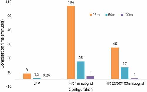
LISFLOOD-FP was about 20 times faster than HEC-RAS for the same grids and time step (computation time for L50 was 1 min 20 s, and for HR50_1 it was 25 min). HEC-RAS of 25-m resolution and 25-m sub-grid terrain are faster than the same resolution with 25-m terrain, but this difference become less evident for large mesh. HEC-RAS of 100-m large mesh and 1-m sub-grid resolution is four times slower than HR100_100, which means that considering high performance (overall extent 78% accuracy and 0.71 m RMSE at watermarks), HR100_1 is the best choice in HEC-RAS simulations. When 1-m sub-grid is implemented in HEC-RAS simulations, the model performs similarly in terms of flood extent (See Table 3); however, the computation time can be drastically decreased by using large mesh (HR100_1). Configuration L25 showed the best performance in terms of flood extent and water depth at selected control points; however, it is two times slower than HR100_1.

5 Discussion

The two codes of different complexity and terrain resolution used in this study strongly affected the quality of the outputs. The diffusion wave model (HEC-RAS) and the inertial formulation of the shallow water equation (LISFLOOD-FP) are distinct in different ways. The ability of HEC-RAS to include the sub-grid bathymetry component makes it effective in terms of representation of topographic details by computing more informative property tables for each cell face. The LISFLOOD model, in turn, operates with the rectangular mesh of the same resolution as the input terrain raster.

5.1 Performance comparison

As was outlined in Section 4, the structured regular mesh of both models is able to reproduce the flooding event with sufficient correspondence to observations and can capture the overall inundation extent and water depth marks at selected watermarks. The mesh size played a great role in the accuracy of the outputs of LISFLOOD-FP; the 25-m grid model performed somewhat better than coarser grids considering the inundation boundary. One of the main reasons for this performance is the ability of the finer resolution models to capture more terrain details and route the flow in the right direction considering depressions and the relief. The flood extent of the 50- and 100-m models (L50 and L100, respectively) were almost similar, differing from each other by only 1% in terms of the measure of fit value, F. The HEC-RAS model, in turn, had comparable results across the resolutions and sub-grid terrain configurations considering flood extent in the whole study area; nevertheless, compared to LISFLOOD-FP (L25), the F value is slightly less accurate. This is of specific importance for areas with complex topography. However, overall differences in extent between the best performing L25 and the rest of the configurations are minimal. This can be explained by the rather confined area, which is shaped by the embankments of the Secchia River from the west and another river from the east; moreover, the northern boundary is also well-pronounced and acts as a barrier to the floodwater preventing it propagating further north. Therefore, we suggest that the terrain configuration explains the similar performance of the models (77–78% accuracy, apart from L25 with 81% accuracy). This also confirms the previous findings that inundation extent over larger areas can be properly identified with low-resolution datasets (in our case 50 or 100 m), with the additional benefit of lower computational costs (Savage et al. 2016). Such findings can be relevant for areas with similar terrain configurations regardless geographical location.

However, as predicted, the behaviour of the models in the focus areas had diverse patterns. For instance, HR50_1 and HR100_1 were able to represent the inundation boundaries in Bomporto fairly well, unlike in Bastiglia (see Figs. 7 and 8), while LISFLOOD-FP was more accurate at high resolution of 25 m compared to 50 and 100 m. The L25 configuration performed strikingly better than HR25_25 both overall and in the two focus areas (i.e. Bomporto and Bastiglia). We explicitly highlight such results, as L25 provided the best outcomes in terms of flood extent and water depth across all selected configurations (see Table 2 and 3). We suggest that this outcome of both models is strongly related to their ability to simulate floods in built-up areas with given resolution. It is known that the towns of Bomporto and Bastiglia are not only represented by urban fabric, being surrounded by a network of smaller channels and embankments, which, in the case of the 2014 flood event, played a crucial role in the inundation dynamics.

One of the similarities between both models is the performance of the 50-m and 100-m LISFLOOD-FP and HEC-RAS models when sub-grid terrain resolutions are not considered for the latter code. For instance, by applying configurations L50 and HR50_50 we attained rather comparable inundation patterns in Bastiglia (Fig. 8) and almost identical patterns in Bomporto (Fig. 7).

The watermark errors evaluated in the current study show how models represented water depth spatially. A point that deserves attention is the vertical accuracy of the input and calibration data. As was discussed earlier, the vertical accuracy of the used LiDAR dataset (±0.15 m) and the observed data (±0.5 m) are a subject of uncertainties. Looking at the differences between observed and simulated watermark values, we suggest that the RMSEs are within the input data error range. However, despite eliminating the outliers, we cannot be 100% confident that the values perfectly match the reality. Therefore, here we treat the results as a relative comparison between the two models rather than compare absolute observed and simulated values. In addition, the points also serve as an indicator to evaluate the simulations, where the watermarks were not inundated. Overall, in terms of RMSE, the HEC-RAS model with 1-m sub-grid terrain for all resolutions was better compared to that with coarser terrains (approx. 0.13 m difference in terms of RMSE between HEC-RAS 1-m sub-grid and coarse sub-grids, including LISFLOOD-FP simulations). The only exception is the 25-m resolution LISFLOOD-FP, which was comparable to the highly detailed sub-grid of HEC-RAS (RMSE of 0.61 and 0.62 m, respectively). We suggest that such performance can be explained by the fact that most of the points are quite a short distance apart (up to 200 m) on heterogeneous terrain, meaning that the water depth points varied by over 1 m. In the Bomporto and Bastiglia focus areas, some points were located within a distance of 30–40 m, which was far denser than the resolution of the underlying terrains (50–100 m). Therefore, HEC-RAS on 1-m sub-grid performed the best due to its ability to operate with highly detailed terrain compared to other configurations with coarse sub-grids (both LISFLOOD-FP and HEC-RAS).

The differences in terms of computation time outlined in Section 4 are crucial, for instance, for calibration and running Monte Carlo simulation scenarios, especially if we intend to extrapolate this performance parameter to the larger-scale studies. Therefore, we suggest that flood mapping for geographically large areas can still be performed with the coarser grids (50 or 100 m) and produce reasonable results to identify the flood-risk hotspots. Such hotspots can be then analysed using high-resolution datasets. In HEC-RAS configurations, the use of a high-resolution (1-m) sub-grid outperforms those with the same resolution as the size of the mesh (25, 50 or 100 m). However, the computational costs for the 1-m sub-grid is higher. The modeller should select among the two options in relation to the mesh size: on the one hand, when the mesh size is small (25 m) the difference in computation time is significant. On the other hand, when the mesh size is larger, the difference in terms of computation time among the two becomes smaller. Use of the 1-m sub-grid becomes more advantageous in terms of computation time, as it additionally shows high performance.

Nevertheless, considering large-scale simulations, we expect that smaller areas that are complicated by highly heterogeneous terrain, but have the potential for large socio-economic impacts (as is the case in Bomporto), will still be misrepresented and wrongly estimated. As shown in the example of this study, the resolution of the topographic description is not the only key factor; another element of paramount importance is the ability of the model mesh/grid to correctly capture critical terrain features which determine the flood wave propagation. This aspect becomes particularly crucial when simulating floods over heavily anthropogenically altered floodplains, as was the case in our study.

The solution of the problem can be assisted by performing a bottom-up assessment, where the most vulnerable and susceptible areas are initially considered in hazard modelling, as was done in the current study. As it was known which areas were impacted the most, we particularly focused on the model behaviour in these regions. It helped us to attain better performance based on the study of Carisi et al. (2018) for the January 2014 event. In probabilistic assessment, these areas can be particularly outlined by intentionally focusing on the locations with high concentration of population/assets, meaning that more attention should be given to analyse flood characteristics in the calibration stage. By doing this, we may reduce uncertainties related to the identification of hotspots.

5.2 Limitations

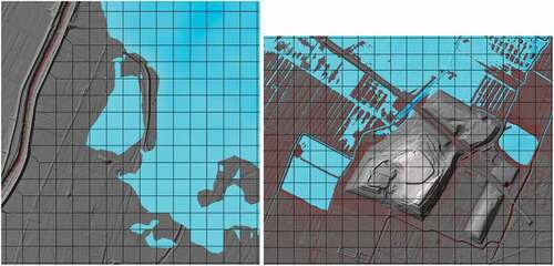
One of the main issues for the HEC-RAS applications is the way in which the model distributes the water within a mesh cell. The volume–elevation curve drawn for each cell-face in pre-processing does not recognize the exact location of the higher/lower ground of the sub-grid terrain. In the case of a rectangular mesh, when the cell faces are not aligned with the elevated linear features, they are not captured in the property tables. Therefore, we may observe a leaking effect (see Fig. 10), or, in contrast, when the model cannot recognize the obstacles for the flow and routes it further onto a neighbouring cell. This is a known limitation, previously observed in the used version of HEC-RAS 5.0 (Goodell 2015). In our case, we noticed that there is a certain amount of hydraulically disconnected flooded areas. Moreover, this effect is particularly obvious in the simulations with coarser sub-grid terrains. However, some areas simulated as flooded (see Fig. 10) are disconnected from the main inundated area. This might be a limitation in the calculation of flood extent and, in some cases, the distribution of local water depth values. This problem is normally solved by refining the mesh with the breaklines, reducing the mesh sizes along such linear irregularities; however, as explained above, the current study did not look into this property.

Figure 10. Leakage effect of HEC-RAS sub-grid mesh examples of HR100_100 (left) and HR25_1 (right). Larger ponds of water in both images are disconnected from the inundation extent.

Inundation boundaries produced by LISFLOOD-FP should be also taken with great care, as the model operates with a raster grid, and the water is distributed equally across the whole cell. For coarse grid resolutions (i.e. pixel size equal to or larger than 100 m), it might thus misestimate the flood extent. In areas with complex topography, it is necessary to include important terrain features into the model. Due to the fact that LISFLOOD-FP simulates four directional water propagations at each cell face (i.e. D4 routing), the linear irregularities captured by L25 configuration (see Fig. 11) would actually be sufficient to limit the flood propagation over such an elevation distribution. We suggest that this simplification of LISFLOOD-FP in the case of high-elevation fine linear terrain features (i.e. levees, embankments (light green cells in Fig. 11) could help to route the water in the right direction and not to allow it to “leak” through the embankments. Nevertheless, the same peculiarity would restrain the water propagation in lower-elevation fine linear terrain features (i.e. rivers, canals, drainage networks) (blue cells in Fig. 11, i.e. the area near Bomporto). The same point applies to the structured grid of HEC-RAS.

Figure 11. Twenty-five-meter resolution DEM. Dark blue: canal, light green: levee.

By having a 25-m mesh cell size (the smallest in this case), it is not always possible to capture important local topographical features, such as embankments, small channels, etc., especially when the linear features are significantly narrower than the model resolution. The known and widely used practice to include the actual terrain heights (levees, embankments, etc.) by “burning” them into the coarser terrain enables such features to be captured, even when their width is smaller than the terrain resolution and mesh size. We intentionally avoided this option to see how the models would respond to the simplified approach of terrain pre-processing. Supposedly, on the geographically larger scale, such manipulation, if the complex and dense network of narrow levees in a specific area are “burnt” in the terrain, may not be always feasible and/or effective. In particular, in cases when such modifications would greatly affect the storage volume of floodplains (i.e. when a 100 m × 100 m raster cell is given the height of the much narrower feature of 10-m breadth). Moreover, this is certainly a challenging task for areas that are not covered by LIDAR data acquisition, as well as areas with poor data availability and quality in general.

6 Conclusions

Due to the specific nature of the event described in this study and the growing use of fully 2D codes for flood modelling, we evaluated and compared the performance of the well-known HEC-RAS and LISLOOD-FP models for a floodplain with a complex and highly anthropogenically altered topography. The aim of the study was to see how the models of different complexity with given terrain resolution would reproduce the flooding event and to establish the accuracy of the results. The resolutions were rather coarse for the given study area, as our main goal was to identify the potential of the codes and mesh dimensions to simulate events over large regions.

One of the conclusions from the study is that 50-m resolution for describing a terrain with complex linear features is a reasonable compromise between output accuracy and computation time for the LISFLOOD-FP model, while for HEC-RAS the optimum solution would be the configuration of 1-m sub-grid terrain and 100-m mesh size. This experience may contribute to simulations performed at catchment scales designed to capture large-scale system behaviour. Specific floodplain morphology may serve as water storage areas during flooding events and, hence, lower the risks in the downstream part of the catchment.

Another point is the complexity of the modelling schemes. The raster-based LISFLOOD-FP model was more efficient at representing overall flood extent and water depth at watermarks, while HEC-RAS performed better at representing spatial distribution details (i.e. inundation boundary) considering given terrain (due to its high-resolution sub-grid feature). Therefore, selection of the modelling scheme and resolution should be carefully considered depending on the purpose of a given case study.

Finally, a topical issue in 2D code usage for large-scale simulations using high-resolution datasets is computational cost. As mentioned above, this can be significantly advanced by using the GPU version of the codes. In this study, we highlight the computational advantage of the inertial formulation of the shallow water LISFLOOD-FP model compared to diffusion wave HEC-RAS. This study shows that codes with simplified physics are a necessary tool for probabilistic/preliminary flood-risk assessment. Moreover, by including high-resolution sub-grid (HEC-RAS with 1-m terrain) we obtain more detailed hazard maps even for large meshes (i.e. 25, 50 or 100 m), albeit sacrificing the computational time. When comparing the overall performance of configuratins L25 and HR100_1, the latter is two times faster; however, L25 showed somewhat better results in flood extent and water depth representation.

Nevertheless, we suggest that more complex tools (i.e. full momentum shallow water codes) have their place in local-scale studies to provide hyper-detailed hydrodynamic modelling. Moreover, future work should consider cases in which the channel flow simulation is included in the model. Such advances will shed more light on the application of 2D models of different complexity.

Disclosure statement

No potential conflict of interest was reported by the authors.

Additional information

Funding

This work was supported by the Marie Sklodowska-Curie Innovative Training Network “A Large-Scale Systems Approach to Flood Risk Assessment and Management – SYSTEM-RISK” [Grant Agreement number: 676027].

References

- Alfieri, L., et al., 2014. Advances in pan-European flood hazard mapping. Hydrological Processes, 28 (13), 4067–4077. doi:10.1002/hyp.9947
- Alfieri, L., et al., 2015. Global warming increases the frequency of river floods in Europe. Hydrology and Earth System Sciences, 19 (5), 2247–2260. doi:10.5194/hess-19-2247-2015
- Alfieri, L., et al., 2017. Global projections of river flood risk in a warmer world. Earth’s Future, 5 (2), 171–182. doi:10.1002/2016EF000485
- Apel, H., et al., 2009. Flood risk analyses – how detailed do we need to be? Natural Hazards, 49 (1), 79–98. doi:10.1007/s11069-008-9277-8
- Arnell, N.W. and Gosling, S.N., 2016. The impacts of climate change on river flood risk at the global scale. Climatic Change, 134 (3), 387–401. doi:10.1007/s10584-014-1084-5
- Aronica, G., Bates, P.D., and Horritt, M.S., 2002. Assessing the uncertainty in distributed model predictions using observed binary pattern information within GLUE. Hydrological Processes, 16 (10), 2001–2016. doi:10.1002/hyp.398
- Bates, P., Horritt, M.S., and Fewtrell, T.J., 2010. A simple inertial formulation of the shallow water equations for efficient two-dimensional flood inundation modelling. Journal of Hydrology, 387 (1–2), 33–45. doi:10.1016/j.jhydrol.2010.03.027
- Bates, P.D. and de Roo, A.P.J., 2000. A simple raster-based model for flood inundation simulation. Journal of Hydrology, 236 (1–2), 54–77. doi:10.1016/S0022-1694(00)00278-X
- Brunner, G.W., 2016. HEC-RAS river analysis system. Hydraulic reference manual. Version 5.0. Davis, CA: Hydrologic Engineering Center.
- Büchele, B., et al., 2006. Flood-risk mapping. Contributions towards an enhanced assessment of extreme events and associated risks. Natural Hazards and Earth System Sciences, 6 (4), 485–503. doi:10.5194/nhess-6-485-2006
- Carisi, F., et al., 2018. Development and assessment of uni- and multivariable flood loss models for Emilia-Romagna (Italy). Natural Hazards and Earth System Sciences, 18 (7), 2057–2079. doi:10.5194/nhess-18-2057-2018
- Castellarin, A., Ceola, S., Toth, E., and Montanari, A. 2014. Evolving water resources systems. In: A. Castellarin, et al., ed. Understanding, predicting and managing water–society interactions. Wallingford, UK: International Association of Hydrological Sciences (IAHS), IAHS Publication, 144–7815, 364.
- Contributors OSM, 2012. OpenStreetMap. Available from: www.openstreetmap.org [Accessed 15 March 2017]
- Coulthard, T.J., et al., 2013. Integrating the LISFLOOD-FP 2D hydrodynamic model with the CAESAR model. Implications for modelling landscape evolution. Earth Surface Processes and Landforms, 38 (15), 1897–1906. doi:10.1002/esp.3478
- D’Alpaos, L., et al., 2014. Relazione tecnico-scientifica sulle cause del collasso dell’argine del fiume Secchia avvenuto il giorno 19 gennaio 2014 presso la frazione San Matteo: Regione Emilia-Romagna, Bologna (Technical-scientific report on the causes of the collapse of the bank of the Secchia River on January 19, 2014 in the San Matteo district: Emilia-Romagna Region, Bologna, in Italian). Available from: http://www.comune.bastiglia.mo.it/files/file/doc_relazione_Secchia_lug14.pdf [Accessed 18 September 2019].
- de Almeida, G.A.M. and Bates, P., 2013. Applicability of the local inertial approximation of the shallow water equations to flood modeling. Water Resources Research, 49 (8), 4833–4844. doi:10.1002/wrcr.20366
- de Moel, H., van Alphen, J., and Aerts, J.C.J.H., 2009. Flood maps in Europe–methods, availability and use. Natural Hazards and Earth System Sciences, 9 (2), 289–301. doi:10.5194/nhess-9-289-2009
- Di Baldassare, G., et al., 2009. Probability-weighted hazard maps for comparing different flood risk management strategies. A case study. Natural Hazards, 50 (3), 479–496. doi:10.1007/s11069-009-9355-6
- Di Baldassare, G., et al., 2010. Flood-plain mapping. A critical discussion of deterministic and probabilistic approaches. Hydrological Sciences Journal, 55 (3), 364–376. doi:10.1080/02626661003683389
- Dimitriadis, P., et al., 2016. Comparative evaluation of 1D and quasi-2D hydraulic models based on benchmark and real-world applications for uncertainty assessment in flood mapping. Journal of Hydrology, 534, 478–492. doi:10.1016/j.jhydrol.2016.01.020
- Domeneghetti, A., et al., 2013. Probabilistic flood hazard mapping. Effects of uncertain boundary conditions. Hydrology and Earth System Sciences, 17 (8), 3127–3140. doi:10.5194/hess-17-3127-2013
- Domeneghetti, A., et al. 2014. Effects of minor drainage networks on flood hazard evaluation. In: A. Castellarin, ed. Understanding, predicting and managing water–society interactions. Wallingford, UK: International Association of Hydrological Sciences (IAHS), IAHS Publication 364, 192–197.
- Domeneghetti, A., et al., 2015. Evolution of flood risk over large areas. Quantitative assessment for the Po river. Journal of Hydrology, 527, 809–823. doi:10.1016/j.jhydrol.2015.05.043
- EC, 2007. Directive 2007/60/EC of the European Parliament and of the Directive 2007/60/EC of the European Parliament and of the Council of 23 October 2007 on the assessment and management of flood risks, Flood Directive, revised European Parliament and Council. In: Official Journal L 288.
- EEA, 2007. CLC2006 technical guidelines. Luxembourg: Publications Office, (Technical report (European Environment Agency.Online), 17/2007).
- Falter, D., et al., 2013. Hydraulic model evaluation for large-scale flood risk assessments. Hydrological Processes, 27 (9), 1331–1340. doi:10.1002/hyp.9553
- Fewtrell, T.J., et al., 2008. Evaluating the effect of scale in flood inundation modelling in urban environments. Hydrological Processes, 22 (26), 5107–5118. doi:10.1002/hyp.7148
- Geoportale Nazionale, 2017. Progetto PST - Dati LiDAR. Available from: http://www.pcn.minambiente.it/mattm/progetto-pst-dati-lidar/ [Accessed 01 February 2018].
- Goodell, C., 2015. The RAS solution 2015. 2D Mesh “Leaking”. Available from: http://hecrasmodel.blogspot.com/search/label/Leaking [Accessed 01 February 2019].
- Haile, A.T. and Rientjes, T.H.M., 2005. Effects of LiDAR DEM resolution in flood modelling. A model sensitivity study for the city of Tegucigalpa, Honduras. ISPRS WG Iii/3, Iii/4, 3, 12–14.
- Hailemariam, F.M., Brandimarte, L., and Dottori, F., 2014. Investigating the influence of minor hydraulic structures on modeling flood events in lowland areas. Hydrological Processes, 28 (4), 1742–1755. doi:10.1002/hyp.9717
- Horritt, M.S., et al., 2010. Modelling the hydraulics of the Carlisle 2005 flood event. Proceedings of the Institution of Civil Engineers - Water Management, 163 (6), 273–281. doi:10.1680/wama.2010.163.6.273
- Horritt, M.S. and Bates, P.D., 2002. Evaluation of 1D and 2D numerical models for predicting river flood inundation. Journal of Hydrology, 268 (1–4), 87–99. doi:10.1016/S0022-1694(02)00121-X
- Hunter, N.M., et al., 2008. Benchmarking 2D hydraulic models for urban flooding. Proceedings of the Institution of Civil Engineers - Water Management, 161 (1), 13–30. doi:10.1680/wama.2008.161.1.13
- Kundzewicz, Z.W., et al., 2013. Flood risk and climate change. Global and regional perspectives. Hydrological Sciences Journal, 59 (1), 1–28. doi:10.1080/02626667.2013.857411
- Lehner, B., et al., 2006. Estimating the impact of global change on flood and drought risks in Europe. A continental, integrated analysis. Climatic Change, 75 (3), 273–299. doi:10.1007/s10584-006-6338-4
- Liu, Z., Merwade, V., and Jafarzadegan, K., 2019. Investigating the role of model structure and surface roughness in generating flood inundation extents using one- and two-dimensional hydraulic models. Journal of Flood Risk Management, 12 (1), e12347. doi:10.1111/jfr3.12347
- Milly, P.C.D., et al., 2002. Increasing risk of great floods in a changing climate. Nature, 415 (6871), 514–517. doi:10.1038/415514a
- Morsy, M.M., et al., 2018. A cloud-based flood warning system for forecasting impacts to transportation infrastructure systems. Environmental Modelling & Software, 107, 231–244. doi:10.1016/j.envsoft.2018.05.007
- Munich Re, 2015. NatCatSERVICE loss events worldwide 1980–2014. Munich, Germany: Munich Reinsurance, 10.
- Neal, J., et al., 2012. How much physical complexity is needed to model flood inundation? Hydrological Processes, 26 (15), 2264–2282. doi:10.1002/hyp.8339
- Néelz, S. and Pender, G., 2013. Benchmarking the latest generation of 2D hydraulic flood modelling packages. Report SC120002. Environment Agency. Environment Agency, Horison House, Deanery Road. Available from: http://publications.environmentagency.gov.uk [Accessed 19 December 2018].
- Orlandini, S., Moretti, G., and Albertson, J.D., 2015. Evidence of an emerging levee failure mechanism causing disastrous floods in Italy. Water Resources Research, 51 (10), 7995–8011. doi:10.1002/2015WR017426
- Sampson, C.C., et al., 2015. A high-resolution global flood hazard model. Water Resources Research, 51 (9), 7358–7381. doi:10.1002/2015WR016954
- Savage, J.T.S., et al., 2016. When does spatial resolution become spurious in probabilistic flood inundation predictions? Hydrological Processes, 30 (13), 2014–2032. doi:10.1002/hyp.10749
- Schumann, G.J.-P., et al., 2009. Progress in integration of remote sensing–derived flood extent and stage data and hydraulic models. Reviews of Geophysics, 47 (4), RG2002. doi:10.1029/2008RG000274
- Schumann, G.J.-P., et al., 2016. Rethinking flood hazard at the global scale. Geophysical Research Letters, 43 (19), 10, 249–10, 256. doi:10.1002/2016GL070260
- Syme, W.J., 2008. 9th National Conference on hydraulics in water engineering. Hydraulics 2008. Barton, ACT: Engineers Australia.
- Tayefi, V., et al., 2007. A comparison of one- and two-dimensional approaches to modelling flood inundation over complex upland floodplains. Hydrological Processes, 21 (23), 3190–3202. doi:10.1002/hyp.6523
- Teng, J., et al., 2017. Flood inundation modelling. A review of methods, recent advances and uncertainty analysis. Environmental Modelling & Software, 90, 201–216. doi:10.1016/j.envsoft.2017.01.006
- Vacondio, R., et al., 2016. Simulation of the January 2014 flood on the Secchia River using a fast and high-resolution 2D parallel shallow-water numerical scheme. Natural Hazards, 80 (1), 103–125. doi:10.1007/s11069-015-1959-4
- Vacondio, R., Dal Palù, A., and Mignosa, P., 2014. GPU-enhanced finite volume shallow water solver for fast flood simulations. Environmental Modelling & Software, 57, 60–75. doi:10.1016/j.envsoft.2014.02.003