Assessing the skill of the UK Hydrological Outlook

ABSTRACT

The UK Hydrological Outlook (UKHO) is a seasonal forecast of future river flows and groundwater levels. The UKHO contains both presentations of outputs from models simulating future conditions and a high-level summary. The summary is produced by an expert panel of forecasters that considers the model outputs together with other recent hydrological and meteorological information. Whilst the skill and uncertainty of the individual models have been explored and published, this study sets out to establish the performance of the high-level summary, and presents such an assessment of the river flow forecasts at the 1-month timescale. Both qualitative and quantitative assessments are presented and compared with two naïve forecasting methods. The UKHO summary is found to have a similar Gerrity skill score to a “same as last month” forecast, an outcome that generates suggestions for improvements in how the different model outputs should be considered and presented in the high-level summary.

KEYWORDS:

• forecasting
• prediction
• modelling
• rainfall
• river flow
• water resources

Editor S. ArchfieldAssociate Editor M. Piniewski

1 Introduction

Seasonal projections of future hydrological conditions have great potential to improve flood and drought forecasting, water resource management, irrigation scheduling and hydropower production. To realize this potential, many countries have developed operational services to deliver such forecasts. These services reflect local circumstances with respect to factors such as river basin characteristics and data availability.

In the UK a Hydrological Outlook (UKHO) has been prepared and disseminated on a monthly basis since the end of 2013 by a team comprised from seven research and operational organizations: the Environment Agency (EA), the Scottish Environment Protection Agency (SEPA), the Department for Infrastructure – Rivers (DfIR) and Natural Resources Wales (NRW), the UK Met Office (MO), and two Natural Environment Research Council centres, the Centre for Ecology & Hydrology (CEH) and the British Geological Survey (BGS). The scientific underpinning and operational delivery of the UKHO is described in Prudhomme et al. (2017).

The UKHO presents forecasts of river flows and groundwater levels that are focussed on the next 1 and 3 months but sometimes extend further into the future. The river flows forecasts are largely based on three modelling approaches, while groundwater level forecasts are generated using two modelling approaches. The published UKHO includes summary outputs from the individual models plus a high-level one-page summary of the available information aimed at a very broad audience, including non-specialists. The production of this high-level summary which is based on a multi-model approach, but also incorporates other information, is a key innovation in seasonal hydrological forecasting.

While the skill of the individual methods is understood there has, to date, been no assessment of the skill of the summary. This is the gap addressed in this paper. In the first instance, the assessment is made only for 1-month-ahead forecasts of river flows. For this reason, there will only be passing references to forecast of groundwater levels in the remainder of this paper.

This assessment directly addresses the most commonly asked question, i.e. How good is the outlook? Until now statements concerning skill have been method specific, and perhaps also site and season dependent.

While this assessment should inform users of future UKHO forecasts, and provide feedback to the UKHO team, it is also anticipated that it will have wider relevance in the production and assessment of other forecasts that combine information from a number of sources using a process that necessarily introduces a measure of subjectivity, albeit based on expert opinion.

This paper is structured as follows: Section 2 describes operational seasonal hydrological forecasts outside the UK; Section 3 gives an overview of the information and methods available to the UKHO, and the elements contained in the summary of the UKHO; in Section 4 there is a description of the methodology used to assess the skill of this summary; and the results are presented in Section 5, with a discussion in Section 6 and concluding remarks in Section 7.

2 Operational seasonal hydrological forecasting service

The UKHO is not the only seasonal hydrological forecast in operation around the globe, and a number of well-established operations already include a performance evaluation of the forecasts.

In Australia, the Bureau of Meteorology has been publishing seasonal streamflow forecasts since 2009, following a long period of drought affecting many regions of Australia. At the outset, the system was based on existing components combined and repurposed to produce seasonal forecasts (Plummer et al. 2009). A brief history of the developments made to date is presented on the Bureau of Meteorology’s website¹ ; these include adding additional forecast locations, changes in the presentation of model results and the updating of assessment and presentation of skill scores. Skill scores are derived from hindcasts derived for the period of record at each site using three measures of goodness-of-fit, or score: continuous ranked probability score (CRPS), root mean square error (RMSE) and RMSE in probability (RMSEP). The skill score (SS) is calculated as:

(1) $\mathrm{S}\mathrm{S}=\left(S_{\mathrm{m}\mathrm{o}\mathrm{d}}-S_{\mathrm{r}\mathrm{e}\mathrm{f}}\right)/\left(S_{\mathrm{p}\mathrm{e}\mathrm{r}\mathrm{f}}-S_{\mathrm{r}\mathrm{e}\mathrm{f}}\right)$(1)

where S_mod is the score for the forecast; S_ref is the score for a reference forecast, e.g. climatology; and S_perf is the score for a perfect forecast which is usually 0 or 1.

To date, the service has been using a statistical approach based on relationships between climate indicators, antecedent catchment conditions, historical rainfall and streamflow to forecast total streamflow in the coming three months. These relationships are site-specific and results have until July 2017 been presented as terciles in pie chart form. The three classes are related to observed historical data for the same three-month period and represent low flows, near median flows and high flows. Each forecast is accompanied by a forecast skill score. Since July 2017 site-specific forecasts have been presented as box-plots.

In addition to the site-specific forecasts, the website also has an overview page containing headlines, a text summary, a map showing all of the sites for which forecasts have been made (with the tercile pie-chart), an overview of the catchment conditions in the previous month, and a brief statement of current climate indices. The tercile pie charts are displayed with an indication of the forecast skill.

As with most forecasting endeavours, this service has been, and continues to be, enhanced and the website notes that new statistical and modelling approaches are the subject of ongoing hydrological research. That merging of forecasts from different methods will be required is acknowledged, but not specifically addressed.

In the USA, the National Weather Service of the National Oceanic and Atmospheric Administration (NOAA) makes seasonal hydrological forecasts available via the Climate Prediction Center (CPC) as US Drought Information.

Information is updated at three timescales: a weekly Drought Monitor presents the current situation and two outlooks provide 1-month and 3-month outlooks. The outlooks have three elements: a map indicating regions in which droughts may be removed, persist or develop; text providing a fairly high-level summary of the latest monthly/seasonal assessment; and a rather fuller discussion giving a region-by-region insight into the information and thinking behind the higher-level information, including a qualitative indication of the confidence of the forecast.

It is interesting to note that the US Drought Information is presented as one of several “expert assessments” by the CPC² alongside other assessments such as the US Hazards Outlook and the Global Ocean Assessment. The CPC seasonal forecasts are quite openly an expert’s synthesis and opinion of all available information and each is attributed to a named forecaster.

There are other services available too, some of which appear to be in a process of continual enhancement. For example, within Europe the European Drought Observatory (EDO³ ) provides a great deal of information to describe the current hydrometeorological status across Europe and the Global Flood Awareness System (GLOFAS⁴ ), which provides hydrological forecasts for a 45-day time horizon. The South Asia Drought Monitor publishes regular updates but with a severe disclaimer and the warning that it is an exploratory research effort.

That this is an active area of ongoing research is evidenced by the recent publication of a special issue of the Hydrology and Earth System Sciences journal containing some 39 papers (Wetterhall et al. 2016).

Whilst a number of hydrological reporting and outlooks systems do exist internationally, the UKHO, we believe, is the only one to bring together a number of different methods and synthesizes these into a summary forecast. The development and application of a method by which to assess the skill of such a summary is the focus of this paper.

3 Methods of river flow forecasting within UKHO

Three modelling approaches are used to forecast future river flows. These methods are based on: analogy and persistence in river flows; seasonal forecasts of rainfall used as input to a hydrological model; and hydrological models driven by historical rainfall ensembles. All three methods deliver forecasts that have zero lead time, i.e. the forecasts when issued relate to the current period.

The method, based on Analogy and Persistence (AP), is described in Svensson (2015). In brief, 1- and 3-month average flow forecasts are made on a site-by-site basis for approximately 94 river gauging stations across the UK. The method generates three forecasts all of which are based only on (standardized) historical flow data.

Two of these are based on historical analogue forecasts, a technique based on the assumption that there are particular trajectories that the hydroclimatic system may follow and that these may be repeated. Analysis of historical data determined that the best analogue duration for a 1-month-ahead forecast was six months, and for a three-month ahead forecast a nine-month analogue duration was best. The analysis did not clearly identify the best number of analogues to use, and the pragmatic decision was made to use five, i.e. roughly 5% of the possible analogues. The two analogue forecasts arise from different methods of averaging the selected analogues: one based on weighted mean and the other on a shifted weighted mean. The third forecast from the AP method is based on persistence alone, i.e. the standardized flow from recent observations will continue for the forecast period.

Forecasts coming from these three methods can be assigned a confidence based on site-specific historical data, and it is the method with the greatest confidence that is given as the single best forecast from the AP method. Forecasts based on persistence are normally preferred to those from analogy. Confidence is generally greatest in the summer in the groundwater-fed catchment in the south-east of the UK; in some months, most often in the winter in the north-west of the UK confidence in the forecasts are too low to justify making a forecast. A standard map-based presentation shows the forecast at all sites used colours to indicate flow magnitude in three classes (above normal, normal and below normal) and symbol size to indicate confidence. Svensson (2015) presents the precision of the forecast using a largely qualitative description of the associated contingency tables and correlations between forecasts and observed data for the hindcast period.

Bell et al. (2017) describe the seasonal rainfall forecast (SRF) method used in the UKHO. SRF uses seasonal forecasts of precipitation produced on an operational basis by the UK Met Office (MacLachlan et al. 2015) to produce a simple water balance model (Bell et al. 2013) which represents the land surface of Great Britain at 1-km resolution. The rainfall forecasts are delivered as a 42-member ensemble of UK-wide (i.e. spatially uniform) standardized totals for 1- and 3-month durations and are downscaled as described in Bell et al. (2007). While the skill of the hydrological forecasts is partly driven by the skill of the rainfall forecast, knowledge of the initial conditions is equally important. These are obtained by running a more sophisticated hydrological model, the Grid-to-Grid (Bell et al. 2009), driven by daily rainfall data at a 5-km resolution to the start of the forecast period; then, the model storages are exported to initiate the simpler water balance model.

In this way, each of the 42 rainfall ensemble members is run through the water balance and produces a (standardized) river flow for every 1 km of Great Britain. These results can be summarized in many ways, but two forms of presentation are generally used, both of which involve regional aggregation corresponding to major drainage basins. One presentation shows the regionally average standardized flow from five members of the rainfall ensemble (lowest, first quartile, median, third quartile and highest) for both 1- and 3-month-ahead forecasts. The other presentation shows the distribution of flow forecasts using a seven-class system (exceptionally low, notably low, below normal, normal, above normal, notably high, exceptionally high).

Neither form of presentation indicates the confidence in the forecasts. However, from Bell et al. (2017) this is known to be highest in the autumn and winter because of the skill in the rainfall forecast at this time of year, for example, 70% of the skill in 3-month-ahead forecast can be attributed to the rainfall forecasts. However, for the 1-month-ahead forecasts 64% of the skill can be attributed to the hydrological initial conditions. Improvements to the SRF method are expected to be delivered by improved resolution in the seasonal rainfall forecasts. This assessment of skill is intended to inform to developers of the method where the skill comes from (i.e. rainfall forecast of hydrological initial conditions) and where they should focus their efforts to improve the method.

The Ensemble Streamflow Prediction (ESP) method of river flow forecasting as implemented for the UKHO is described by Prudhomme et al. (2017). As with the SRF method rainfall inputs are used to drive hydrological models to forecast future conditions. However, in the ESP method, the inputs come from 51 historical sequences of precipitation and potential evapotranspiration, and the hydrological modelling is catchment based. The use of historical sequences enables modelling to extend further into the future, in this case twelve months, although all forecasts are averaged over this time frame and are therefore zero lead-time forecasts. Three hydrological models have been used: GR4J (Perrin et al. 2003), PDM (Kay et al. 2006) and Classic (Crooks and Naden 2001).

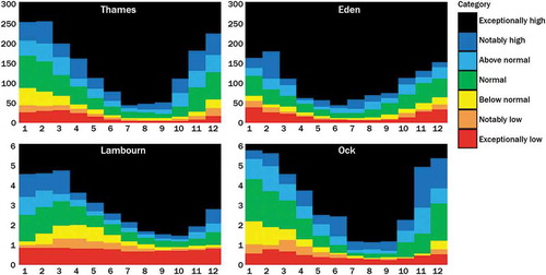
Results are presented in two ways. The first is similar to the histograms used by the SRF method, i.e. the same seven-class system is used but each histogram represents a site rather than a region. The second form of presentation is a stack diagram that shows how the distribution changes with time out to 12 months. This latter presentation is particularly useful visualizing the return to normal from an above, or more normally, a below normal situation.

As with the SRF method, there is no formal statement of the confidence of any of the forecasts over any duration. However, Harrigan et al. (2017) have investigated the skill of the ESP method in the UK, but use a different rainfall-runoff model to the one used by the UKHO for the period covered in the assessment presented in this study.

As might be expected the skill was found to vary with forecast duration, starting month, and catchment properties. In summary, forecasts for groundwater-dominated catchments that are for periods that include summer months are generally more skilful. The skill score (SS) used is as previously presented with mean square error and CRPS used as the measure of goodness-of-fit.

Each monthly forecast is provided with the outputs from these three methods. It is obviously helpful that the three methods all base their presentations on the same classification system, albeit with different numbers of classes. However, the methods use different methodologies (i.e. they are three hydrological models driven by the same data or one hydrological model driven by three different datasets). The way they present confidence differs too; only one (AP) presents this as part of the forecast, for the other two this is contained in background material.

For each of the methods some assessment of skill, or perhaps more accurately performance, has been undertaken, but with each taking its own approach. This diversity in assessment methodology also extends to the groundwater level forecasts for which skill is assessed using bias, reliability, and relative operating characteristic (ROC) score, and CRPS skill scores. Thus while the developers of the different methods have each made their own assessment of their method’s performance there is no standard method used to provide a skill score.

3.1 Categorization of river flows

Each forecast of river flows is assigned to a category using the same classification as adopted for the UK’s Hydrological Summary and by the National Hydrological Monitoring Programme. This classification scheme (see Table 1) has seven classes with a central class that represents “normal”. As can be seen, these classes are not set on the basis of equal probability; the normal class represents 44% of all river flows, and the size of the classes decreases towards both extremes. This scheme is used in different ways in the three models contributing to the UKHO: the SRF method preserves all seven classes of this scheme, whereas ESP uses a reduced scale with five classes, and in AP only three classes are used. The choice of how many classes to use reflects different approaches adopted by the developers of the methods. Providing seven classes may not be justified by the method’s performance but the user can decide how classes might be combined for their particular use of the forecast. At the other extreme by presenting forecasts in only three classes the developer is clearly indicating what they consider to be the reliable level of discrimination that the method can provide.

Table 1. Classification scheme for forecasts of river flows, reproduced from Prudhomme et al. (2017).

Since all of the underpinning methods refer back to this classification it is worth exploring in slightly more detail what is meant by normal and how it varies between catchments and with the season. The scaling of river flows is desirable to remove factors such as catchment size and average rainfall from the forecasts, and makes the forecast very accessible to the reader, as everyone has an intuitive idea of what is meant by normal. The UK is fortunate to have many long hydrological records and can use these data to derive the boundaries between the classes. This set of class boundaries, therefore, contains considerable information about the statistics of monthly flow rates. Without such long records, these boundaries would be poorly defined, and an alternative scaling between catchment might be required such as scaling by catchment area.

In the UK there is a considerable variation in river flow regimes as a consequence of climatic and catchment characteristics. The seasonal variation is driven in some places by the seasonal distribution of rainfall. However, in a large part of the UK rainfall is relatively uniform throughout the year, and the variation in river flows is the consequence of rainfall exceeding evaporation in the winter months, whereas in the summer, evaporation exceeds rainfall. Added to this there is the variation in soil and geology, which influence the storage of water within catchments. Four river flow regimes derived from at least 40 years of observed data illustrate this variation (Fig. 1). In all four catchments, there is considerable seasonal variation in river flows, with the classes shrinking in absolute magnitude from winter to summer. The Eden and the Thames have roughly similar flow volumes, but while the Thames has a catchment area approximately four times that of the Eden, the Thames receives much less rainfall. The Ock and the Lambourn are neighbouring catchments within the basin of the Thames with almost identical catchment areas, and yet the flows differ in magnitude, and in the timing of the seasonal peaks and troughs, because although climatic drivers are very similar the Ock contains impermeable soils with low storage, and the Lambourn permeable soils with high storage.

Figure 1. Four river flow regimes derived from at least 40 years of observed data.

The class boundaries derived from long data records, therefore, have embedded within them all of the characteristics that determine the flow regime. It is all too easy to gloss over the amount of information content behind stating that in a particular month, a river’s flow falls within a particular probability class.

3.2 Production process of the UKHO and its summary

In terms of generating each monthly forecast, the methods have their different data requirements: AP requires the previous month’s river flow data; ESP requires the previous month’s rainfall data; SRF requires the previous month’s rainfall and the forecasts of future rainfall. The UKHO is produced on a calendar month basis and has the objective of posting each month’s outlook as early as possible. In practice, the delivery is constrained by the availability of the data. Perhaps surprisingly the forecasts of future rainfall are the first data to be available and are normally supplied by the MO on around the 24th of the previous month. Monthly rainfall data are generally available on around the third working day of the month and river flows by day six.

Running the three hydrological models has become a routine and straightforward task, and so the Forecasters’ Meeting is scheduled for around the sixth working day of the month. As well as considering the model outputs the meeting takes regard of the observed river flows from the end of the previous month, and provisional observed rainfall data for the month to date. The observed river flows are coordinated and presented by the UK Hydrological Summary. The meeting also welcomes any other relevant information that any of the project partners can provide to help inform the outlook, e.g. information relating to any of the observed underpinning data, or additional model forecasts.

The designated author for the summary usually coordinates all of this information and will highlight areas where the available information is in good agreement, and areas of disagreement. The latter, of course, is more problematic and it is necessary to consider if disagreement means uncertainty, or whether information from particular sources or models should be given more or less weight. Some methods have greater skill levels at particular times of year and recognizing this is a key consideration. Once the general message is agreed there is a discussion about key messages and what might appear on the summary map, i.e. are there regional differences that can be simply displayed in map form. The relationship between what appears on the map, and how this might be qualified in the accompanying text, is a particular concern: it is known that the map is sometimes separated from the text as the summary is relayed and further digested by user groups.

After due consideration of all of these factors, the author prepares the summary using a standard template with the following components.

• Summary: a high-level overview containing key messages about the hydrological conditions in the month ahead (~100 words).

• Rainfall: a brief note on last month’s rainfall and text supplied by the MO about the rainfall forecast (~120 words).

• River flow: a brief commentary on last month’s river flows and the current forecast (~120 words).

• Groundwater: A brief commentary on last month’s groundwater levels and the current forecast (~120 words).

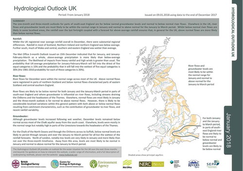
• Map: a map that gives a simplified visualization of regional variations in the forecast.

The summary page is then circulated to all project partners for comments, corrections and sign-off. An example of the summary page is presented in Fig. 2.

Figure 2. Summary page from the January 2018 Hydrological Outlook.

It should be appreciated that only rarely does the information contained in the summary use more than the three classes: above normal, normal and below normal. This partly represents the (low) confidence the models have in discriminating at the extremes of the scales and partly because there have been no long-lasting extreme events since the UKHO went into routine production, i.e. since 2014. Should more extreme conditions occur, e.g. similar to those experienced in 2013, it may be that five or seven classes of the full classification are used.

It is, of course, almost impossible for long-lasting flood flows to occur in the relatively small catchments of the UK. The UKHO cannot forecast floods as in the UK these are always the consequence of short duration rainfall events. Sustained above normal flows can occur, and did in early 2014, but while these conditions indicate that while further heavy rainfall may lead to flood, they are not flood forecasts. Extreme low flow events are more likely but have not arisen during the operational lifetime of the UKHO.

4 A methodology for skill assessment

The three modelling approaches have all separately published information concerning the performance and/or skill of their predictions. These evaluations are generally in the conventional form of objective goodness-of-fit statistics. The challenge in assessing the skill of the summary is that it is not presented numerically.

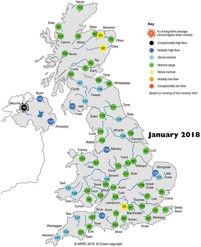
There is, however, a readily available source of validation data: the monthly river flows data for up to 100 river gauging stations published in the Hydrological Summary for the United Kingdom (HS), in the form presented in Fig. 3. These are 1-month mean river flows so, therefore, would enable a skill assessment over that period.

Figure 3. Monthly river flow data from the Hydrological Summary for January 2018.

The textual information in the summary of the UKHO refers to areas of the UK, some of which are well defined e.g. Scotland and Northern Ireland. Other regional descriptions are more ambiguously defined, for example, East Anglia could refer to the NUTS2 region (second tier of Nomenclature of Territorial Units for Statistics) or a slightly larger area commonly thought of as East Anglia that also includes Essex. It could also be confused with the Environment Agency East Anglia Region, which was based on river catchment boundaries rather than administrative regions.

The authors of the summary are in fact quite content with this level of uncertainty in their text since they know that there are no hard boundaries or cut-offs in their forecasts. While the map contains relatively little information it does provide clear geographical zoning. It should perhaps be appreciated that in considering how information is added to the map there was some debate as to whether the lines should be made wider or blurred to help convey the uncertainty. It was though decided to keep the lines as thin and hard-edged and rely on warnings in the text and the common sense of readers to understand that they should not be taken as hard boundaries.

Nevertheless, for the purpose of this assessment the method adopted was to compare the summary map with the point river flow data from the HS. For each station presented on the HS map, the class shown for the same location on the summary map of the UKHO was abstracted, so that at each point there was an observed and forecast class. As the UKHO only uses three classes the data from the HS were also merged into the corresponding three classes.

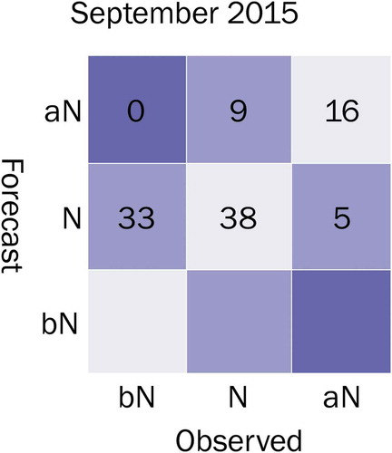
For each month a three by three contingency table was derived in which the observed classes were compared with the forecast classes (Fig. 4). Ideally, the data would fall in the bins on the diagonal from bottom left to top right indicating perfect correspondence between observation and forecast. Data above and below this diagonal are imperfect forecasts, with the top left and bottom right bins which represent situations in which the forecast was for above normal, yet the observation was below normal, or vice versa.

Figure 4. Example of the contingency table for September 2015.

In the remainder of this paper the abbreviations aN, N and bN are used for above normal, normal and below normal respectively.

For September 2015 the Outlook forecast was for N flows in 76% of rivers and aN flows in 25% of rivers, with no bN flows. Observed flows fell into all three categories 33% bN, 47% N and 21% aN. All data were abstracted as numbers of occurrences and converted to percentages as the actual number of observations varied from month to month. Percentages were rounded to the nearest integer and rounding errors can mean that the totals do not add to 100%. The zero in the top left represents a value that has been rescaled to zero, whereas in the blank squares there were no data.

There are, however, many occasions in which the author of the UKHO indicates even more vagueness in the forecast by suggesting that the river flows may be “normal to above normal” or “normal to below normal”.

This was the case in May 2015 (Fig. 5(a)), in which the forecast was for 38% of river flows to be normal and 62% to be “normal to below normal”. To remove this non-symmetrical aspect from the contingency table it was decided to allocate such forecast equally to the two basic classes as shown in Fig. 5(b).

Figure 5. Contingency tables for May 2015: (a) N-bN forecast included, and (b) with N-bN forecast allocated equally to N and bN categories.

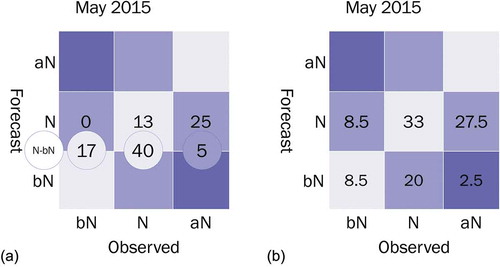
Following this procedure, data were abstracted into 24 contingency tables for the months from September 2014 to August 2016, i.e. roughly equivalent to two water-years. These contingency tables provide a visual (qualitative) way to assess the performance of the summary, i.e. bigger numbers in the lighter coloured bins imply better performance, whereas numbers in the darker coloured bins suggest worse performance. An objective (quantitative) method of assessing the skill from the contingency tables is presented below.

Table 2 shows the contingency table based on the whole evaluation period; it reveals that in 2% of cases (approximately 50 instances from a total of 2400) the prediction was for aN when bN flows occurred, or vice versa.

Table 2. Contingency table for the whole evaluation period (September 2014–August 2016).

	Observed
Forecast	bN	N	aN
bN	4	4	1
N	11	38	22
aN	1	8	11

The frequencies presented in Table 2 are expressed as the percentage, P_ij, of occurrences for forecast (outlook) category j (j = 1, …, 3) and observed category i (i = 1, …, 3), and are readily converted to relative sample frequencies p_ij.

Before moving on to the objective method of assessment, the representativeness of the evaluation period can be explored. Table 3 shows the expected percentage of aN, N and bN values, the observed and forecast percentages for the two years individually and the entire period, i.e. the sum of P_ij over j and i respectively.

Table 3. Summary of monthly flows by class during the assessment period showing the “expected” distribution, the distribution of observations and the distribution of the forecasts.

		Observed			Forecast
	Expected	2014/15	2015/16	2014–2016	2014/15	2015/16	2014–2016
bN	28	18	12	15	14	8	11
N	44	57	46	51	78	62	70
aN	28	25	41	33	8	30	19

Comparing the expected and actual probabilities, the year 2014/15 is “more normal” than expected, 2015/16 has very many more aN flows than expected, and so for the period as a whole, the observed data are shifted towards aN flows.

The forecast probabilities are very much biased towards N which is most likely to reflect caution on behalf the forecaster to opt for an unambiguous aN or bN: remember that both the aN and bN forecast may in fact come from the case in which the forecast is for flows to be “normal to above (below) normal”.

Analysis of the contingency table is covered comprehensively by Jolliffe and Stephenson (2003), as part of an extensive manual for techniques for “Forecast Verification”. There are a surprisingly large number of metrics that can be derived from the contingency table including the hit rate (or probability of detection), bias, proportion correct, accuracy, sensitivity and specificity. It is undoubtedly the case that the different metrics may provide different relative scores and therefore provide more confusion than enlightenment. Jolliffe and Stephenson recommend the Gerrity skill score (GSS) for the type of three-category ordinal data available in this study. The GSS is also the World Meteorological Organization’s recommended skill score for three-by-three contingency tables associated with long range forecast verification (WMO 2010). On the basis of these endorsements the GSS has been the adopted as the sole metric for use in this study.

Jolliffe and Stephenson (2003) and WMO (2010) give the background to their recommendations and only a brief overview is provided here. The GSS uses a scoring matrix s_ij which specifies the reward or penalty corresponding to each of the p_ij in the contingency table, thus:

(2) $\mathrm{G}\mathrm{S}\mathrm{S}={\sum }_{i=1}^K{\sum }_{j=1}^K{p}_{ij}{s}_{ij}$(2)

The values s_ij are straightforwardly calculated using formulae contained in both the above references. The GSS has several desirable features notably the use of all information in the contingency table, penalizing larger error more than smaller errors, and providing greater rewards for correct forecasts of infrequent events. The GSS is also said to be equitable giving values of zero for random forecasts and constant forecasts of any single category.

The scoring matrix corresponding to the data in Table 3 is presented in Table 4. The symmetrical nature of the scoring matrix is a feature of the Gerrity scoring matrix, as is the fact that s₁₃ = s₃₁ = – 1. In this example the reward for the correct forecast aN or bN are roughly three and nine times greater respectively then for a correct N forecast.

Table 4. Gerrity scoring matrix corresponding to the contingency table for the whole evaluation period (September 2014–August 2016).

	Observed
Forecast	bN	N	aN
bN	3.035742	–0.25373	–1
N	–0.25373	0.335891	–0.41038
aN	–1	–0.41038	1.104774

The WMO (2010) guidance is that at least 90 forecast/observation pairs are required to properly estimate the contingency table. The monthly data used here would be close to this limit and so we have adopted the WMO guidance to aggregate the data from the 24 monthly contingency tables into seven datasets representing three time periods and the four seasons. GSS values are presented in Table 5 for these seven datasets.

Table 5. Gerrity skill scores for the three periods and four seasons for the UKHO forecasts and two naïve methods.

	Outlook forecast	ALWN	SALM
2014–2016	0.174	0.000	0.242307
2014/15	0.068	0.000	0.294559
2015/16	0.236	0.000	0.189393
Autumn	0.141	0.000	0.161013
Winter	0.189	0.000	0.170226
Spring	0.070	0.000	0.08098
Summer	0.158	0.000	0.236117

5 Results

For all seven datasets the GSS is greater than zero but with a range from 0.068 to 0.236. The skill of the forecasts in 2015/16 was very much better than in 2014/15, because of greater success in correctly forecasting above normal flows in the later period. Of the four seasons, forecasts for summer, winter and autumn are equally skilful, but those made for spring are noticeably poorer. During spring 66% of observed flows were N (the highest N percentage in the seven datasets), and two-thirds of these were correct, it is a feature of the GSS that a constant forecast (e.g. always N) will result in GSS of zero even if always correct.

To provide some context to evaluate the GSS derived from the UKHO forecast, two extremely simple alternatives have been included. The first to consider is an “always-normal” (ALWN) forecast which we already know will give a GSS of zero, so just represents an example of a forecast that will have a GSS of zero. The second is “the-same-class-as-was-observed-last-month” (SALM), i.e. the forecast at a site was for the same class as was observed in the previous month.

Looking at all of the datasets the actual forecast is always better than the constant forecast of ALWN (restating what we already know), but the SALM forecast is roughly equivalent to, or better than the actual forecast. The success of SALM seems to come from the summer months during which the skill of the actual forecast drops. Neither the actual forecast nor SALM give much greater skill than ALWN in spring.

There is a noticeable different between the GSSs for the two years. The skill of the actual forecast is much lower than SALM in 2014/15, which we have already seen is more normal than expected. In contrast the skill scores for 2015/16 show the actual forecast to be somewhat better than SALM, and it is notable that this is the only one of the seven datasets for which this is the case. This outcome is a consequence of the actual forecast correctly forecasting some aN flows that a SALM will miss.

6 Discussion

An obvious starting point for discussion is that the SALM forecast appears to be as good as, or even slightly better than, the actual forecast. This is perhaps even harder to understand when one of the methods (AP) used to inform the actual forecast is based on what might be considered an enhanced form of SALM. There are a number of possible reasons for this outcome.

Firstly, the AP method may not be given sufficient weight when the summary forecast is being prepared, i.e. the other methods may be seen as more sophisticated and therefore containing more valuable information. The forecasters, therefore, might do well to consider last month’s actual flows, or the AP forecasts as a good starting point, and consider what evidence the other methods bring to suggest a different outcome.

Secondly, the SALM approach allows for a site-by-site forecast, whereas the actual forecast has hard regional boundaries. These boundaries may be qualified in the accompanying text, for example to suggest a particular forecast is applicable to groundwater-fed catchments, but this information has been lost in undertaking this skill assessment. As a reminder of how different the flow regime can be in neighbouring catchments consider again the monthly flow regimes presented in Fig. 1 for the Ock and Lambourn. These two catchments would almost always be in the same region in the summary map yet have very different flow regimes as a consequence of very different soils and geology.

Thirdly, it is necessary to remember that the SALM forecast is not for the same flow as last month, but for the same class of flow as last month and therefore contains the information built into to the flow regime plots presented in Fig. 1. While SALM is an apparently simple forecasting method it actually has the class trajectories embedded within it and thus reflects the catchment characteristics and driving climatic variables.

Another noticeable feature is the lack of skill in the spring. The UKHO forecasters are aware of how relatively small differences in both initial conditions, i.e. the amount of water stored in river basins, and climate, mainly rainfall and temperature, can have a large impact on the trajectory of future river flows at this time of year.

It was recognized above that conservative forecasts, i.e. forecasts for N, can reduce the skill score, whereas correct aN or bN forecast boost the skill score. This raises the issue of the level of boldness that should be built into the summary of the UKHO, i.e. is it better to err on the side of caution and opt for a N forecast, or be bolder and indicate aN or bN even without overwhelming evidence that this will occur? Anecdotal evidence from users suggests a greater level of boldness is the preferred approach, but those producing the UKHO do not want to be seen as producing unjustified, attention-grabbing, sensational forecasts.

The fact that the 2-year period used to assess the skill of the UKHO summary contained more months with N and aN flows than expected, and therefore fewer bN flows, combined with the difference in skill scores between the two years implies that a longer period should be considered to better quantify the skill of the summary map.

However, extending the assessment period is not without complications as there have been changes in the process of producing the UKHO summary. Some of these are easily recognized, such as there being a better understanding of the skill of each of the methods that contribute to UKHO. Other changes are less tangible, for example, what changes may have been introduced through the very experience of producing the UKHO and from informal feedback from users. Indeed undertaking this assessment of the skill of the UKHO will no doubt change the way the different outputs are assessed and combined.

7 Conclusion

Seasonal forecasts are produced on a routine basis in many countries, and the importance of indicating the skill associated with the forecast is widely recognized. This is straightforward for forecasts that are based on a single method, but more complicated where the forecast from several methods are integrated into an overview or summary. Providing a summary of this type seems to be a unique aspect of the UKHO, and therefore presents a new challenge when assessing its skill.

A method of assessing the skill has been developed and implemented for the two year period from September 2014. The method compares the map from the UKHO with a map prepared by the Hydrological Summary for the UK and therefore does not integrate the messages from the accompanying text with what is presented on the map, so to a degree may be seen as an unfair assessment. Nevertheless, the method allows an objective assessment based on the GSS which is a recommended metric for the skill assessment of categorical ordinal seasonal weather forecasts.

It has been shown that if only the information from the map in the summary of the UKHO is considered this provides a forecast that is roughly equivalent in its skill to a same-class-as-last-month forecast, but better than a random forecast or a constant forecast of, say, always normal flows. The unanswered question is whether the accompanying information e.g. the text that sits alongside the map brings extra skill to the forecasts. If this is the case, then the UKHO may well be improved by revisiting the way in which the summary is presented, i.e. moving away from a simple zoned map as a way of delivering the key messages of the summary.

The skill assessment methodology presented here provides a baseline which will enable a future review to quantify future changes in the overall skill of the UKHO.

The message to users of the UKHO is that, like all forecasts, there is a lot of uncertainty. They should not rely on the summary map alone but note the accompanying text. Users might also consider diving into the underlying data and model forecasts as perhaps there is information more relevant to their need. Making it easier to “drill-down” into this information may make this a more attractive option.

Finally, this very open assessment of the skill contained within the UKHO summary can be easily adopted in each of the methods on which the summary is based, and in other countries to assess their high-level products. Indeed a highly desirable outcome of this study would be for the GSS to be widely adopted to assess the skill of hydrological seasonal forecasts. It would be interesting to see how skill levels compare between different regions, climates, hydrological settings and methods. Using a single skill metric would surely benefit both those developing seasonal hydrological forecasts and users of the forecasts.

Acknowledgements

The research described in this paper is based on the forecasts provided by the partnership that delivers the UK Hydrological Outlook, as already described, and in particular the contributions of Nuria Bachiller-Jareno, Vicky Bell, Helen Davies, Jamie Hannaford, Shaun Harrigan, Alan Jenkins, Simon Parry, Christel Prudhomme, Ali Rudd, Katie Smith and Cecilia Svensson. The authors gratefully acknowledge their contributions. The views expressed in this paper are those of the authors and do not necessarily reflect those of the organization that employs them. The authors also gratefully acknowledge the very constructive comments of the reviewers of the first draft of this manuscript.

Disclosure statement

No potential conflict of interest was reported by the authors.

Additional information

Funding

This work was supported by the Natural Environment Research Council award number NE/R016429/1 as part of the UK-SCAPE programme delivering National Capability.

Notes

¹ http://www.bom.gov.au/water/ssf/history.shtml.

² http://www.cpc.ncep.noaa.gov/products/expert_assessment/.

³ http://edo.jrc.ec.europa.eu/edov2.

⁴ http://www.globalfloods.eu/.

References

- Bell, V.A., et al., 2007. Development of a high resolution grid-based river flow model for use with regional climate model output. Hydrology and Earth System Sciences, 11 (1), 532–549. doi:10.5194/hess-11-532-2007
- Bell, V.A., et al., 2009. Use of soil data in a grid-based hydrological model to estimate spatial variation in changing flood risk across the UK. Journal of Hydrology, 377 (3–4), 335–350. doi:10.1016/j.jhydrol.2009.08.031
- Bell, V.A., et al., 2013. Developing a large-scale water-balance approach to seasonal forecasting: application to the 2012 drought in Britain. Hydrological Processes, n/a–n/a. doi:10.1002/hyp.9863
- Bell, V.A., et al., 2017. A national-scale seasonal hydrological forecast system: development and evaluation over Britain. Hydrology and Earth System Sciences, 21 (9), 4681–4691. doi:10.5194/hess-21-4681-2017
- Crooks, S.M. and Naden, P.S., 2001. CLASSIC: a semi-distributed rainfall-runoff modelling system. Hydrology and Earth System Sciences, 11 (1), 516–531. doi:10.5194/hess-11-516-2007
- Harrigan, S., et al., 2017. Benchmarking ensemble streamflow prediction skill in the UK. Hydrology and Earth System Sciences Discussions, 1–28. doi:10.5194/hess-2017-449
- Jolliffe, I.T. and Stephenson, D.B., 2003. Forecast verification: a practitioner’s guide in atmospheric science. Chichester, West Sussex, England: J. Wiley.
- Kay, A.L., et al., 2006. A comparison of three approaches to spatial generalization of rainfall-runoff models. Hydrological Processes, 20 (18), 3953–3973. doi:10.1002/(ISSN)1099-1085
- MacLachlan, C., et al., 2015. Global Seasonal forecast system version 5 (GloSea5): a high-resolution seasonal forecast system. Quarterly Journal of the Royal Meteorological Society, 141 (689), 1072–1084. doi:10.1002/qj.2396
- Perrin, C., Michel, C., and Andréassian, V., 2003. Improvement of a parsimonious model for streamflow simulation. Journal of Hydrology, 279 (1–4), 275–289. doi:10.1016/S0022-1694(03)00225-7
- Plummer, N., et al., 2009. A seasonal water availability prediction service: opportunities and challenges. In: 18th World IMACS/MODSIM Congress, 13–17 July 2009 Cairns, Australia, 13–17.
- Prudhomme, C., et al., 2017. Hydrological Outlook UK: an operational streamflow and groundwater level forecasting system at monthly to seasonal time scales. Hydrological Sciences Journal, 62 (16), 2753–2768. doi:10.1080/02626667.2017.1395032
- Svensson, C., 2015. Seasonal river flow forecasts for the United Kingdom using persistence and historical analogues. Hydrological Sciences Journal, 61 (1), 19–35. doi:10.1080/02626667.2014.992788
- Wetterhall, F., et al., eds, 2016. Sub-seasonal to seasonal hydrological forecasting. Hydrology and Earth System Sciences, https://www.hydrol-earth-syst-sci.net/special_issue824.html
- World Meteorological Organization, 2010. Attachment II.8: standardized verification system (SVS) for long-range forecasts (LRF). In: Manual on the global data-processing and forecasting system. Volume I – global aspects. Geneva: World Meteorological Organization.