A multi-model ensemble approach for the assessment of climatic and anthropogenic impacts on river flow change

ABSTRACT

Climate variability and human activities are considered to be the most likely reasons for negative trends in river inflow and the water level of some lakes and wetlands in the world. To quantify the uncertain impacts of climate variations and anthropogenic activities on Ajichay River flow in Iran, a multi-model ensemble approach based on the Bayesian model averaging (BMA) method is applied. Several statistical and simulation-based methods are used to distinguish the impacts of climatic and anthropogenic factors on river flow. The results show that almost all the methods identified human activities as the dominant impact on streamflow (about 73–85% of the change). The between-model and within-model uncertainty analyses using BMA showed that the 95% uncertainty intervals of the individual approaches have relatively large deviation ranges. The BMA mean prediction could reduce the range of between-model uncertainties to 14–27% for climate impacts and 74–80% for human impacts. This approach provides a way to better understand the contributions of climatic and anthropogenic impacts on river flow change.

KEYWORDS:

• climate impacts
• human activities
• Bayesian model averaging
• SWAT model
• uncertainty

Editor Ross WoodsAssociate editor M. Piniewski

1 Introduction

In the last decade, negative trends in the river inflow and water level of multiple lakes and other waterbodies have introduced different challenges. Various climate factors (e.g. climate change and continuous droughts) and human-induced changes (e.g. land-use changes and dam construction) have been reported as driving forces of this reduction (Raeisi et al. 2018). For instance, there has been a sudden decline in the water level of Lake Urmia, Iran (Jalili et al. 2016) and in the Ajichay streamflow as one of the main rivers flowing to the lake. Not all researchers agree on the contributions of different driving forces of desiccating Lake Urmia such that there is high degree of uncertainty in the identification of basin responses to natural and anthropogenic factors. AghaKouchak et al. (2015) found human activities as the main cause for the desiccation of the lake, while Shadkam et al. (2016a) concluded that about 60% of this change was caused by climate factors and only 40% is related to human activities. Therefore, it is an important issue to realize the impacts of different driving forces of streamflow change considering the uncertainties to help the decision makers to manage the water resources, optimally.

The methods to analyse the hydrological responses to environmental changes are mainly divided into two groups: statistical and simulation-based methods. Different statistical methods such as ecohydrological approach (Wang et al. 2013, Ye et al. 2013, Huang et al. 2014), SCRAQ/SCRCQ (Wang et al. 2012a, 2012b, 2015, Huang et al. 2016), and climate elasticity method (Chen et al. 2013, Ahn and Merwade 2014, Guo et al. 2014, Xia et al. 2014, Zhao et al. 2015, Huang et al. 2016) are widely used by researchers. These methods are mainly based on statistical analysis of relationships between the observed meteorological and hydrological data. Meanwhile, simulation-based techniques, such as conceptual hydrological modelling (Chang et al. 2014, Khoi and Suetsugi 2014, Hu et al. 2015, Niraula et al. 2015, Tan et al. 2015, Cong et al. 2017), multi-regression (Wang et al. 2012a, Ma et al. 2014) and artificial neural network (ANN) (Liu et al. 2010, Tang et al. 2014), are based on analysis of the driving force impacts using a calibrated hydrological model. Since the aforementioned methods apply different procedures to estimate the impacts of climatic and anthropogenic impacts, there would be limitations and uncertainties associated with the structure of the methods, their inputs and assigned parameters. Although hydrological modelling methods provide more detailed outputs for hydrological analysis, there are some limitations in setup and calibration of the models due to lack of data in poorly gauged regions. Moreover, the statistical methods provide less information on hydrological cycle but those are more flexible methods in the case of limited data (Li et al. 2016). Therefore, the application of both statistical and hydrological modelling methods together could be an appropriate approach for the assessment of climatic and anthropogenic impacts on river flow. Moreover, to determine which of these techniques represents the real basin status and to compare them, further assessment of the methods and the analysis of uncertainties sources is required. In this regard, an ensemble method such as Bayesian model averaging (BMA) (Hoeting et al. 1999, Ajami et al. 2006), Bagging (Breiman 1996), or Boosting (Valiant 1984, Schapire 1990) is useful for offering better and more reliable results because of its ability in evaluating in both within- and between-model uncertainties.

In this study, the impacts of climate variability and anthropogenic activities on river inflow changes considering uncertainties of different statistical and simulation-based approaches were quantified. As a main innovation, a multi-model ensemble approach applying the BMA method was used for combining within- and between-model uncertainty of multiple results from different separation methods. This approach can help to better understand the uncertain changes in river flow as a response to human activities and climate variations, which is one of the most important concerns for sustainable water resources management. The proposed approach was applied in the Ajichay River Basin as one of the main catchments of the Urmia Lake Basin in Iran which is facing a significant decline in river flow.

2 Study area

Lake Urmia, the second largest extreme salt lake in the world and the largest lake in Iran, has faced a significant water level and area decline in recent years. To test our approach, the basin of Ajichay River (covering about 20% of the Lake Urmia drainage basin), which is one of the main rivers flowing into the lake, was selected as the study area. This river basin, with an area of 10 304 km², leis between 37º39′–38º28′ E and 45º26′–47º50′ N. Smallholder agriculture dominates the watershed. Figure 1 illustrates the location of the Ajichay River Basin and the spatial distribution of the synoptic, hydrometric and rainfall stations, as well as diversion dams.

Figure 1. Ajichay river basin and its watersheds, sub-basins (from 1 to 36), and stations.

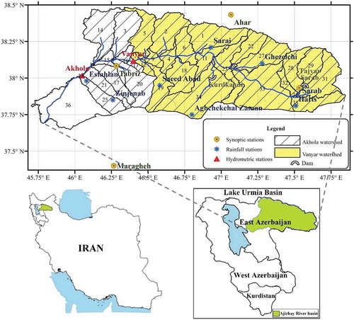
As shown in Table 1, there has been development of both agricultural and domestic areas from 1976 to 2007. The data in Table 1 are based on the information given by Fathian (2012), Fathian et al. (2013) and land-use maps of the area. Furthermore, land-use changes and construction of multiple diversion dams in this river basin might be the main driving forces in changing the river flow.

Table 1. Change in land-use area (km²) in the Ajichay river basin (1976–2007).

Land use	1976	1989	2002	2007
Saltmarsh	51	17	226	388
Rangeland	5783	5319	4750	3641
Irrigated agriculture	152	388	540	761
Rain-fed agriculture	172	648	932	1316
Orchards	69	84	275	303
Mountainous and fallow areas	4078	3849	3582	3896

Based on available datasets, daily temperature data of four synoptic stations, daily rainfall data of three synoptic stations and seven rain gauges, and daily discharge data of Vanyar and Akhola hydrometric stations (obtained from the Water Resources Management Company, Iran) for the period 1987–2007 were applied in this study (Fig. 1). To calculate the average value of these parameters, the Thiessen polygon method was applied. Figure 2 illustrates the graphs of time series of the hydro-climatological variables, including annual precipitation, annual potential evapotranspiration (PET; Thornthwaite 1948), mean annual temperature and annual streamflow.

Figure 2. Time series of hydroclimatological variables: (a) annual precipitation (mm); (b) annual potential evapotranspiration (PET, in mm); (c) mean annual temperature (°C); and (d) mean annual streamflow (m³ s⁻¹).

3 Methods

The methodological approach followed in this study is given in Fig. 3. Here, the trend analysis was carried out using the Mann-Kendall (MK) test (Mann 1945, Kendall 1975) and determination of the change point in a time series was done using the Pettitt test (Pettitt 1979). To identify the climatic and anthropogenic impacts on streamflow, four widely used statistical techniques – double mass curve, rainfall–runoff relationship, water balance method and slope variation – and two hydrological modelling methods – the Soil and Water Assessment Tool (SWAT) conceptual model and an artificial neural network (ANN) data-driven model – were applied. These methods were chosen considering the previous studies as well as their various properties. The assumptions, as well as advantages and disadvantages of the applied methods to distinguish the impacts of climate and human activities on river flow are provided in Table 2. These data are mostly based on the information given by Renner et al. (2012) and Wang (2014).

Table 2. Assumptions, strengths and weaknesses of different methods for the quantification of climatic and anthropogenic impacts on streamflow. SCRAQ, slope change ratio of accumulative quantity; BP-ANN, back-propagation artificial neural network; P, precipitation; PET, potential evapotranspiration.

Method	Assumptions and additional information	Advantages	Disadvantages
TS09	No need to find the changing point Zero deep groundwater losses	Simplicity and application for any region	Inability to quantify the climate and human impacts Annual temporal resolution and not taking more details Not recommended when long-term P ~ = long-term PET
Climate elasticity model	Requires a change point No storage changes and deep groundwater losses during baseline/altered period Rainfall–runoff equation independent of climate (the equation changes only by human activities) Negligible human activities during baseline period	Quantification of the impacts	Taking a fixed model parameter for the whole period which depends only on human activities Annual temporal resolution and not taking more details
SCRAQ	The independent variable: year The dependent variable: cumulated runoff–rainfall Negligible human activities during baseline period	Quantification of the impacts	Annual temporal resolution and not taking more details
Conceptual hydrological modelling	Requires a changing point Requires land-use/cover, soil, management data Negligible human activities during baseline period	Quantification of the impacts Simulating seasonal changes Calculating water storage changes	Time-consuming model calibration and validation Complexity of the model High uncertainty of model parameters
Black-box hydrological modelling approach	Requires a change point Negligible storage changes and deep groundwater losses Negligible human activities during baseline period	Quantification of the impacts Training the model based on observed data	High uncertainty of the results due to the complexity of applied equations and layers

Figure 3. Assessment framework of climatic and anthropogenic impacts on river flow change.

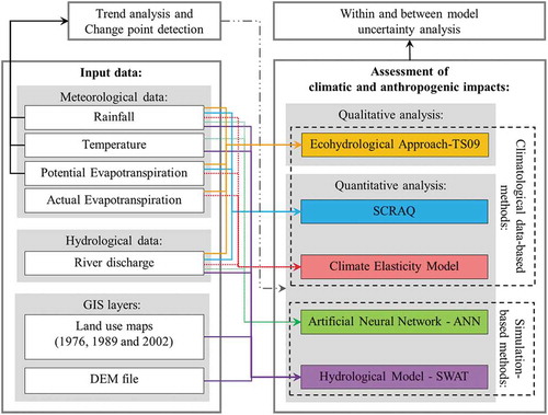
As shown in Table 2, the considered approaches have different strengths in considering various aspects of human and climate impacts on hydrological processes. Also, as they take different parameters and approaches to separate the impacts of climate and anthropogenic activities on river flow, different (but relatively close) results would be achieved. Therefore, a multi-model ensemble approach, that analyses the parameters and structure uncertainties, can present a better performance than any individual model. In this regard, the BMA method was used to combine and perform uncertainty analysis of multiple results of separation techniques. The description of the methods applied to separate the impacts of anthropogenic and climatic impacts on river flow change, as well as the BMA method, are given below.

3.1 Statistical methods

3.1.1 Tomer and Schilling method (TS09)

The Tomer and Schilling (2009) method, also known as TS09, is able to quantify the relative impacts of climate versus human activities on the hydrology of a river basin (Wang 2014). The framework of this method (Fig. 4) is based on the following two formulas:

(1) $P_{\mathrm{e}\mathrm{x}}=\frac{P-AET}{\mathrm{P}}$(1)

(2) $E_{\mathrm{e}\mathrm{x}}=\frac{\mathrm{P}\mathrm{E}\mathrm{T}-\mathrm{A}\mathrm{E}\mathrm{T}}{\mathrm{P}\mathrm{E}\mathrm{T}}$(2)

Figure 4. A conceptual model of eco-hydrological shifts in response to climate variability and land-use change (Tomer and Schilling 2009). P_ex: unused water; E_ex: excess energy; PET: potential evapotranspiration.

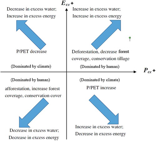
where P, PET and AET represent precipitation, potential evapotranspiration and actual evapotranspiration (calculated by subtracting streamflow from precipitation), respectively. These indicators can be calculated for comparing various desired periods and do not need to detect a change point to divide the time series data into two datasets. The interpretation of the changes in E_ex and P_ex was explained by Wang et al. (2013).

3.1.2 Climate elasticity model for$\mathrm{\Delta }{Q}_{\mathrm{c}}$

The climate elasticity model calculates the contribution of climate variability to streamflow change, which is the weighted mean of precipitation and potential evapotranspiration changes (Wang 2014). In this model, change in streamflow due to climate variations ($\mathrm{\Delta }{\mathrm{Q}}_{\mathrm{c}}$) is expressed as:

(3) $\mathrm{\Delta }{Q}_{\mathrm{c}}=\frac{\mathrm{\partial }Q}{\mathrm{\partial }P}\left(\mathrm{\Delta }P\right)+\frac{\mathrm{\partial }Q}{\mathrm{\partial }\mathrm{P}\mathrm{E}\mathrm{T}}\left(\mathrm{\Delta }\mathrm{P}\mathrm{E}\mathrm{T}\right)={\epsilon }_p\left(\mathrm{\Delta }P\right)+{\epsilon }_{\mathrm{P}\mathrm{E}\mathrm{T}}\left(\mathrm{\Delta }\mathrm{P}\mathrm{E}\mathrm{T}\right)$(3)

where ∆P is the change in precipitation between the altered (after change point) and baseline (before change point) periods, ∆PET is the change in PET between changed and baseline periods; ${\epsilon }_p$ is the rate of change in the river flow associated with precipitation and ${\epsilon }_{\mathrm{P}\mathrm{E}\mathrm{T}}$ is the rate of change in river flow due to PET (Wang 2014).

In this research, a differential climatic elasticity analysis based on the model proposed by Zhang et al. (2001) was used, in which it is assumed that the storage changes during both baseline and changed periods are zero:

(4) $\mathrm{A}\mathrm{E}\mathrm{T}=\left(\frac{1+w\varphi }{1+w\varphi +{\left(\varphi \right)}^{-1}}\right)\times P$(4)

where w is an empirical parameter associated with plant water use and land cover (soil conditions), which is known as the parameter of watershed characteristics (Wang 2014) and usually ranges from 0.5 to 2 (Wang et al. 2013) and $\varphi =\mathrm{P}\mathrm{E}\mathrm{T}/P$ is the baseline period aridity index (Zhang et al. 2001). This equation is calibrated to obtain w for the baseline period. The precipitation and potential evapotranspiration change rates (${\epsilon }_P$ and ${\epsilon }_{\mathrm{P}\mathrm{E}\mathrm{T}}$) are calculated as follows:

(5) ${\epsilon }_P=\frac{1+2\varphi +3w\varphi }{{\left(1+\varphi +w{\varphi }^2\right)}^2}$(5)

(6) ${\epsilon }_{\mathrm{P}\mathrm{E}\mathrm{T}}=-\frac{1+2w\varphi }{{\left(1+\varphi +w{\varphi }^2\right)}^2}$(6)

In this study, Microsoft Excel 2013 was used to calculate the contribution of climate variability to streamflow change using the climate elasticity model.

3.1.3 Slope change ratio of accumulative quantity (SCRAQ)

The slope change ratio of accumulative quantity (SCRAQ) is another climatological data-based method in this regard (Wang et al. 2012b). The slope change rate of the accumulative streamflow ($R_{\mathrm{S}\mathrm{Q}}$, %) is calculated by:

(7) $R_{\mathrm{S}\mathrm{Q}}=100\times \frac{S_{Q.a}-S_{Q.b}}{S_{Q.b}}=100\times \left(\frac{S_{Q.a}}{S_{Q.b}}-1\right)$(7)

where $S_{Q.b}$ and $S_{Q.a}$ (both in 10⁸ m³/year) represent, respectively, the slope of the linear function of year and the accumulative streamflow before and after a change point. Also, $S_{P.b}$ and $S_{P.a}$ (both in mm/year) are, respectively, the slope of the linear function of year and the accumulative precipitation before and after the change point. Now, $R_{\mathrm{S}\mathrm{P}}$ (%), or the slope change rate of the accumulative precipitation, is expressed as:

(8) $R_{\mathrm{S}\mathrm{P}}=100\times \frac{S_{P.a}-S_{P.b}}{S_{P.b}}=100\times \left(\frac{S_{P.a}}{S_{P.b}}-1\right)$(8)

Finally, the streamflow change associated with precipitation ($\mathrm{\%}{\eta }_P$) is estimated as:

(9) $\mathrm{\%}{\eta }_P=\frac{R_{\mathrm{S}\mathrm{P}}}{R_{\mathrm{S}\mathrm{Q}}}\times 100$(9)

By considering $\mathrm{\%}{\eta }_{\mathrm{P}\mathrm{E}\mathrm{T}}$ as the slope change ratio of the linear function of year and accumulative potential evapotranspiration in a river basin, $\mathrm{\%}{\eta }_h$ (the human activities contribution to the streamflow change) is estimated by (Wang et al. 2012b):

(10) $\mathrm{\%}{\eta }_h=100-\mathrm{\%}{\eta }_C=100-\left(\mathrm{\%}{\eta }_P+\mathrm{\%}{\eta }_{\mathrm{P}\mathrm{E}\mathrm{T}}\right)$(10)

This technique, which also carried out in Microsoft Excel 2013, is capable of considering the impact of each of the climatic variables.

3.2 Simulation-based methods

3.2.1 Conceptual hydrological modelling (SWAT)

In this study, a hydrological modelling approach based on the SWAT conceptual model is used as a simulation-based approach for separation of climate and human activity on river flow.

The SWAT model is a continuous and process-based simulation model, which is commonly applied to simulate different hydrological conditions in various scales (Gassman et al. 2007). In this study, the model prepared by Ghodousi (2012) was applied and modified for the purposes of this study.

There have been no large reservoir dams in the basin during the simulation period (1987–2007); however, two small diversion dams (with a total storage capacity of 8.7 × 10⁶ m³; million cubic metres, or MCM) were constructed (Fig. 1) and are considered in the model. Both of these dams have been in operation since 2003.

The effects of dynamic land-use change on river flow are simulated using the land-use update option in SWAT. Details of the hydrological modelling using SWAT, including input datasets and layers, calibration and validation procedures and results, are provided in the Appendix.

After model calibration (1987–1999) and validation (2000–2009), the three following scenarios (Table 3) were defined to calculate the climate and human impacts on streamflow: (a) detrended climatic parameters and observed land use (to reflect only the anthropogenic impacts); (b) original observed climatic parameters with invariable baseline land use and the constructed dams removed (to consider only the impact of climate variation); and (c) original observed data. The baseline period (before the change point) was 1987–1996 for Akhola and 1987–1997 for Vanyar. The impacts were quantified based on the following formulae and defined variables given in Table 3.

(11) $\mathrm{\Delta }{Q}_{\mathrm{c}}={\bar{Q}}_a^{\mathrm{i}\mathrm{n}\mathrm{v}}-{\bar{Q}}_b^{\mathrm{o}\mathrm{b}\mathrm{s}}$(11)

(12) $\mathrm{\Delta }{Q}_{\mathrm{h}}={\bar{Q}}_{\mathrm{a}}^{\mathrm{d}\mathrm{e}\mathrm{t}}-{\bar{Q}}_{\mathrm{b}}^{\mathrm{o}\mathrm{b}\mathrm{s}}$(12)

Table 3. The three scenarios considered in the SWAT model.

Time period	Scenario
	Detrended climatic parameters	Invariable land use and removed dams	Observed
Baseline period (before change)	${\bar{Q}}_{\mathrm{b}}^{\mathrm{d}\mathrm{e}\mathrm{t}}$	${\bar{Q}}_{\mathrm{b}}^{\mathrm{i}\mathrm{n}\mathrm{v}}$	${\bar{Q}}_{\mathrm{b}}^{obs}$
Altered period (after change)	${\bar{Q}}_{\mathrm{a}}^{\mathrm{d}\mathrm{e}\mathrm{t}}$	${\bar{Q}}_{\mathrm{a}}^{\mathrm{i}\mathrm{n}\mathrm{v}}$	${\bar{Q}}_{\mathrm{a}}^{\mathrm{o}\mathrm{b}\mathrm{s}}$

Q, streamflow; det, detrended; inv, invariable; obs, observed; b and a, before and after the change point, respectively.

where ${\bar{Q}}_{\mathrm{a}}^{\mathrm{i}\mathrm{n}\mathrm{v}}$ represents the simulated streamflow discharge obtained from the “invariable land use and removed dams” scenario after the change point; ${\bar{Q}}_{\mathrm{a}}^{\mathrm{d}\mathrm{e}\mathrm{t}}$ is the “modelled streamflow discharge derived from the detrended data” scenario; and ${\bar{Q}}_{\mathrm{b}}^{\mathrm{o}\mathrm{b}\mathrm{s}}$ represents the “original” scenario (observed flow) before the change point (i.e. the baseline period).

To calculate the total change in streamflow value and to compare the sum of $\mathrm{\Delta }{Q}_{\mathrm{c}}$ and $\mathrm{\Delta }{Q}_{\mathrm{h}}$ with $\mathrm{\Delta }\mathrm{Q}$ the following equation was also applied:

(13) $\mathrm{\Delta }\mathrm{Q}={{\bar{Q}}_{\mathrm{a}}}^{\mathrm{o}\mathrm{b}\mathrm{s}}-{{\bar{Q}}_{\mathrm{b}}}^{\mathrm{o}\mathrm{b}\mathrm{s}}$(13)

where $\mathrm{\Delta }Q$, ${{\bar{Q}}_{\mathrm{b}}}^{\mathrm{o}\mathrm{b}\mathrm{s}}$ and ${{\bar{Q}}_{\mathrm{a}}}^{\mathrm{o}\mathrm{b}\mathrm{s}}$represent the total streamflow change, the baseline average streamflow and the changed period average streamflow, respectively.

3.2.2 Black-box hydrological modelling approach (ANN)

The artificial neural network (ANN) is a widely used black-box hydrological modelling approach (Liu et al. 2010) and data-driven simulation-based method. It is a useful method to model the complex relationships between the input layer and the output layer (Tang et al. 2014). In this approach, the change in the streamflow is calculated by Equation (14); the total change in streamflow is associated with both the climate variability and human activities:

(14) $\mathrm{\Delta }Q=\mathrm{\Delta }{Q}_{\mathrm{c}}+\mathrm{\Delta }{Q}_{\mathrm{h}}$(14)

where $\mathrm{\Delta }{Q}_{\mathrm{c}}$ is the streamflow change due to climate variations and $\mathrm{\Delta }{Q}_{\mathrm{h}}$ represents the change in streamflow as a result of human activities.

After training the ANN model for the baseline period, it is run to simulate the average streamflow for the changed period (${\bar{Q}}_{\mathrm{c}\mathrm{a}}$). The change in streamflow associated with the climate variations $\mathrm{\Delta }{Q}_{\mathrm{c}}$ is calculated by subtracting the baseline period streamflow (${\bar{Q}}_{\mathrm{b}\mathrm{a}}$) from ${\bar{Q}}_{\mathrm{c}\mathrm{a}}$:

(15) $\mathrm{\Delta }{Q}_{\mathrm{c}}={\bar{Q}}_{\mathrm{c}\mathrm{a}}-{\bar{Q}}_{\mathrm{b}\mathrm{a}}$(15)

According to Tang et al. (2014), the percentage of climate and human impacts on streamflow can be calculated by:

(16) $\mathrm{\%}{\eta }_{\mathrm{c}}=\frac{\mathrm{\Delta }{Q}_{\mathrm{c}}}{\mathrm{\Delta }Q}\times 100$(16)

(17) $\mathrm{\%}{\eta }_{\mathrm{h}}=\frac{\mathrm{\Delta }{Q}_{\mathrm{h}}}{\mathrm{\Delta }Q}\times 100=100-\mathrm{\%}{\eta }_{\mathrm{c}}$(17)

This technique, like the climate elasticity model, is capable of quantifying the impacts of different climatic variables, depending on how the user defines the input layers.

3.3 Bayesian model averaging (BMA)

The BMA method (Hoeting et al. 1999) is a statistical technique that is efficient for the quantification of within-model and between-model uncertainty (Ajami et al. 2006). The basic ideas of this method are as follows:

The quantity Y is assumed to be simulated on the basis of input data D, and F=(f1, f2, …, fk) is the vector of the K model predictions. The probabilistic prediction of BMA is given by:

(18) $\mathrm{P}\left(Y|D\right)=\sum _{k=1}^K\mathrm{P}\left(f_k|D\right).{\mathrm{P}}_k(Y|f_k.D)$(18)

where P(f_k|D) is the posterior probability of the kth prediction f_k, given the input data D, which shows how well the kth prediction model fits the observed data. For P(f_k|D) the BMA weight of the kth prediction is w_k. A higher weight denotes the better performance of predictions with respect to others. ${\mathrm{P}}_K\left(Y|f_k.D\right)$is the conditional probability density function of the Y conditional on f_k and D. The BMA mean prediction is a weighted average of the model results, with their posterior probabilities being the weights. If the model predictions and observations are all normally distributed, the BMA mean prediction can be shown as:

(19) $\mathrm{E}\left[Q|D\right]=\sum _{k=1}^K\mathrm{p}\left(f_k|D\right).\mathrm{E}\left[{\mathrm{p}}_k(Q|f_k.D)\right]=\sum _{k=1}^K{w}_k{f}_k$(19)

The uncertainty of the BMA mean prediction includes the between-model uncertainty and the within-model uncertainty that can be expressed, respectively, as:

(20) $\mathrm{B}\mathrm{e}\mathrm{t}\mathrm{w}\mathrm{e}\mathrm{e}\mathrm{n}\mathrm{m}\mathrm{o}\mathrm{d}\mathrm{e}\mathrm{l}\mathrm{u}\mathrm{n}\mathrm{c}\mathrm{e}\mathrm{r}\mathrm{t}\mathrm{a}\mathrm{i}\mathrm{n}\mathrm{t}\mathrm{y}=\sqrt{\sum _{k=1}^K{w}_k{\left(f_k-\sum _{i-1}^K{w}_i{f}_i\right)}^2}$(20)

(21) $\mathrm{W}\mathrm{i}\mathrm{t}\mathrm{h}\mathrm{i}\mathrm{n}\mathrm{m}\mathrm{o}\mathrm{d}\mathrm{e}\mathrm{l}\mathrm{u}\mathrm{n}\mathrm{c}\mathrm{e}\mathrm{r}\mathrm{t}\mathrm{a}\mathrm{i}\mathrm{n}\mathrm{t}\mathrm{y}=\sqrt{\sum _{k=1}^K{w}_k{{\sigma }_k}^2}$(21)

In this study, the expectation-maximization algorithm (Moon 1996) is used to estimate the model prediction variance (${\sigma }_k$) and BMA weights ($w_k$) based on the normal posterior distribution of K model predictions. After estimation of the BMA parameters (${\sigma }_k$ and $w_k$), the BMA probabilistic ensemble predictions are generated based on the Monte Carlo method (Metropolis and Ulam 1949). In this regard, the prediction uncertainty interval can be constructed by the Monte Carlo sampling method from the normal distribution with the mean and the variance of each model prediction. BMA probabilistic ensemble predictions are also generated based on $w_k$ of each model. The 95% uncertainty intervals of each model and the BMA approach can be derived based on the ascending order of ensembles within the range of the 5% and 95% quantiles.

In this study, the R package “ensembleBMA” (Fraley et al. 2011) was used for implementing the BMA approach.

4 Results

4.1 Trend and change point analysis

According to Zhang et al. (2012), finding historical trends of hydrometeorological parameters facilitates understanding of the impacts of climate variability on water resources systems. Taking p= 0.05 and 0.1 as the statistically significant levels, the non-parametric Mann-Kendall trend test method was applied to analyse the change trends in annual precipitation, mean temperature, PET and streamflow (1987–2007) for each station and watershed. The magnitude of the trend was estimated by the Kendall tau method.

According to the test results (Table 4), annual precipitation showed no significant trend in the study watersheds, except one station that had a decreasing and the other an increasing trend. The annual mean temperature increased significantly in Akhola watershed, while it showed an increasing trend in Vanyar watershed at the significance level of 10% and no trend at the significance level of 5%. Likewise, PET tended to increase significantly during the 21-year period. In contrast to the temperature and PET, the streamflow significantly decreased.

Table 4. Annual trend analysis of the climatic parameters. Bold indicates Vanyar and Akhola sub-basins. Gridded cells: positive impact on streamflow; grey shaded cells: negative impact on streamflow. PET: potential evapotranspiration; Q: streamflow; +: positive trend; – : negative trend; 0: no trend.

Parameter	Station	Kendall’s tau	p value	Trend
				5%	10%
Precipitation	Sarai	0.248	0.126	0	0
	Esfahlan	0.2	0.22	0	0
	Saeed Abad	–0.2	0.22	0	0
	Aghchekehal Zaman	0.371	0.019	+	+
	Ghezelchi	0.048	0.789	0	0
	Haris	–0.495	0.001	–	–
	Sarab	0.124	0.456	0	0
	Ahar	–0.076	0.655	0	0
	Zinjenab	0.148	0.365	0	0
	Tabriz	0.019	0.929	0	0
	Vanyar	0.04	0.84	0	0
	Akhola	0.02	0.93	0	0
Temperature	Ahar	0.267	0.098	0	+
	Maragheh	0.495	0.001	+	+
	Sarab	0.2	0.22	0	0
	Tabriz	0.39	0.013	+	+
	Vanyar	0.27	0.1	0	+
	Akhola	0.5	0	+	+
PET	Ahar	0.248	0.126	0	0
	Maragheh	0.495	0.001	+	+
	Sarab	0.267	0.098	0	+
	Tabriz	0.381	0.016	+	+
	Vanyar	0.34	0.03	+	+
	Akhola	0.34	0.03	+	+
Q	Vanyar	–0.33	0.037	–	–
	Akhola	–0.36	0.023	–	–

Bold indicates Vanyar and Akhola sub-basins. Gridded cells: positive impact on streamflow; grey shaded cells: negative impact on streamflow.

PET, potential evapotranspiration; Q, streamflow; +, positive trend; –, negative trend; 0, no trend.

As can be understood from the above results, the climate in the Ajichay River basin has become drier and warmer; however, the annual precipitation showed no distinct trend.

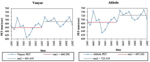
In order to detect the change points in annual mean temperature, PET and streamflow series for Vanyar and Akhola watersheds in the period 1987–2007, the non-parametric Pettitt test was applied (Figs. 5–7). The results show that there was a change point in these variables in the late 1990s (around 1997), with a significance level of p = 0.05, except for the temperature at Vanyar, for which the change point was in 1994. It is also shown that the change point in streamflow across the Vanyar watershed occurred in 1997, while the change point in the Akhola watershed was detected in 1996.

Figure 5. Results of the Pettitt test for annual streamflow series in Vanyar and Akhola (mu1 and mu2: mean annual flow during baseline and altered periods, respectively).

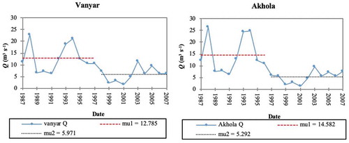
Figure 6. Results of the Pettitt test for annual mean temperature series in Vanyar and Akhola (mu1 and mu2: mean annual temperature during baseline and altered periods, respectively).

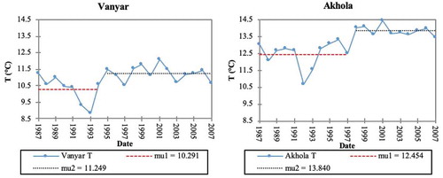
Figure 7. Results of the Pettitt test for annual PET series in Vanyar and Akhola (mu1 and mu2: mean annual PET during baseline and altered periods, respectively).

4.2 Separating climate and human impacts on streamflow using statistical methods

4.2.1 TS09 method

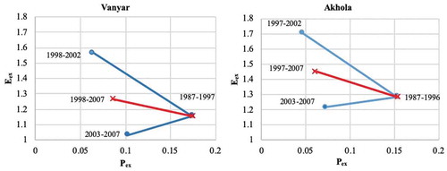
Figure 8 shows the eco-hydrological properties of the watershed in terms of E_ex and P_ex. First, these two indicators were computed for annual data. Since there was no trend in the graph of annual data, they were averaged in sub-periods, in which a pattern was detected. Defining the sub-periods, as mentioned earlier, is based on the objectives of the study. Here, the datasets were divided according to the change point in each sub-basin. The reference period (1987–1997 and 1987–1996 for Vanyar and Akhola, respectively) was compared with the first analysis period (1998–2002 and 1997–2002, respectively). Based on the results, a slight decrease was observed in average P_ex (which is an indicator of a decrease in streamflow) and an increase in average E_ex was noticed. The results obtained for this sub-period show that the impacts of land-use change and climate variability are about equal. Also, when the reference period was related to 2003–2007, a small decrease in both averages of P_ex and E_ex was seen, which is an indication of greater human impacts than the climatic effects. Comparing the reference period with the whole changed period, a minor increase in E_ex and a reduction in P_ex was obtained, which suggests that the main cause of the change in streamflow is due to the climate variability, rather than human impacts.

Figure 8. Results of TS09 (P_ex: unused water, E_ex: excess energy).

4.2.2 Elasticity-based analysis

As mentioned earlier, w is a constant in the elasticity-based model with the highest effect on model outputs; it is the most sensitive model parameter, as can be understood from the governing equations. Parameter w can be calibrated based on the results estimated by the water balance in the natural period (Bai et al. 2014). The results from the elasticity-based analysis are summarized in Table 5. Compared with the reference period 1987–1996 (1997) for Akhola (Vanyar), $\bar{Q}$ for the changed period reduced by 6.8 and 9.3 m³ s⁻¹ for Vanyar and Akhola, respectively. This result is mainly explained by the land-use change (contributing 76.0% and 75.6% of the $\bar{Q}$ change in Vanyar and Akhola, respectively) with the climate variability corresponding to the remaining 24.0% and 24.4% of $\bar{Q}$ change (Table 5). The results from the elasticity-based analysis do not agree with those from TS09 (Section 4.2.1).

Table 5. Summary of the results of different methods for separation of human and climate impacts on streamflow.

Method	Watershed	Model parameter			∆Q	∆Qc	∆Qh	Climate impact	Human impact
		w	Φ			(m^3 s^−1)	(m^3 s^−1)	(%)	(%)
Elasticity_based approach	Akhola	0.912	2.131		–9.289	–2.262	–7.027	24.4	75.6
	Vanyar	0.86	1.984		–6.814	–1.638	–5.176	24.0	76.0
BP–ANN	Akhola	–			–9.289	–2.431	–6.858	26.2	73.8
	Vanyar	–			–6.814	–1.781	–5.033	26.1	73.9
		RSQ	RSP	RSPET
SCRAQ	Akhola	–64.366	–6.505	5.803	–9.289	–1.776	–7.513	19.1	80.9
	Vanyar	–51.755	–5.092	4.922	–6.814	–1.318	–5.496	19.3	80.7
SWAT	Akhola	–			–9.289	–1.012	–7.895	10.9	85.1
	Vanyar	–			–6.814	–0.763	– 5.917	11.2	86.8

BP-ANN, back-ropagation artificial neural network; SCRAQ, slope change ratio of accumulative quantity; SWAT, Soil and Water Assessment Tool. w,: watershed characteristics parameter; Φ = PET/P,: aridity index for the baseline period; P, precipitation; PET, potential evapotranspiration; R_SQ, R_SP and R_SPET, slope change rate of accumulative Q, P and PET, respectively; ∆Q, change in streamflow; ∆Q_c and ∆Q_h, change streamflow change caused by climate variations and as a result of human activities, respectively.

Climate and human contributions to the change in streamflow, as well as the calibrated parameters, are shown in Table 5. The obtained w values are 0.86 (Vanyar) and 0.91 (Akhola). Since the absolute value of the sensitivity coefficients of streamflow to precipitation is greater than the sensitivity coefficients of streamflow to PET in both watersheds, it can be stated that the change in streamflow was more sensitive to precipitation than to PET.

4.2.3 SCRAQ method

Based on the results of the Pettitt test, the periods 1987–1996 and 1997–2007 for Akhola and 1987–1997 and 1998–2007 for Vanyar were considered as the baseline period and the changed period, respectively.

The slope of the linear relationship of the accumulative streamflow decreased by 2.10 × 10⁸ and 2.96 × 10⁸ m³ year⁻¹, with corresponding rates of 51.8% and 64.4% in Vanyar and Akhola, respectively. The slope reduction of the linear relationship of the accumulative precipitation was 17.2 and 21.0 mm year⁻¹, and the decrease rates were 5.1% and 6.5% in Vanyar and Akhola, respectively. In addition, the slope of the linear relationship of the accumulative PET increased by 32.3 and 39.5 mm year⁻¹, at rates of 5.0% and 5.8% in Vanyar and Akhola, respectively. The calculated $\mathrm{\%}{\eta }_{\mathrm{P}}$ using Equation (19) was 9.8% and 10.1% for Vanyar and Akhola, respectively, while the corresponding $\mathrm{\%}{\eta }_{\mathrm{h}}$ using Equation (20) was 80.6% and 80.9%, respectively (because $\mathrm{\%}{\eta }_{\mathrm{P}\mathrm{E}\mathrm{T}}$ was 9.5% and 9.0%, and therefore $\mathrm{\%}{\eta }_{\mathrm{c}}$ was 19.3% and 19.1% for Vanyar and Akhola, respectively). Contributions of climate variability and human activities to the decreased streamflow in Vanyar are 19.3% and 80.6% for the changed period, respectively. The corresponding values for Akhola are 19.1% and 80.9% (Table 5).

4.3 Separating climate and human impacts on streamflow using simulation-based methods

4.3.1 Conceptual hydrological modelling approach

To evaluate the impacts of climate variations and human activities, the calibrated SWAT model for Ajichay River Basin was run for three scenarios, as mentioned above, and the monthly river inflow at the catchment outlets for the period 1987–2007 was simulated. In order to find$\mathrm{\Delta }{Q}_{\mathrm{c}}$, the observed flow during the baseline period was subtracted from the simulated flow in the invariable land-use scenario for the changed period. Afterwards, $\mathrm{\Delta }{Q}_{\mathrm{h}}$ was calculated using the difference between the changed period streamflow in the detrended scenario and the baseline observed streamflow. The mean annual streamflow time series for the observed, detrended and invariable land-use scenarios are shown in Fig. 9. Accordingly, $\mathrm{\%}{\eta }_{\mathrm{c}}$ and $\mathrm{\%}{\eta }_{\mathrm{h}}$ for Vanyar watershed are 10.9% and 85.1%, respectively, while the corresponding values for Akhola watershed are 11.2% and 86.8%. These results show more intense human impacts on streamflow in comparison with the other methods (Table 5).

Figure 9. Mean annual streamflow time series for the observed, detrended and invariable land-use scenarios.

4.3.2 Black-box hydrological modelling approach (BP-ANN)

In this approach, a back-propagation ANN (BP-ANN) was used for black-box simulation of the streamflow using climate variables. Monthly precipitation and temperature were used as inputs to the BP-ANN. The model in the baseline period was trained and tested using the baseline streamflow data. The monthly streamflow datasets for 102 months (8.5 years) and 30 months (2.5 years) were utilized to, respectively, train and validate the BP-ANN model in Vanyar and Akhola watersheds (Fig. 10). The training and validation of the proposed BP-ANN model were performed using MATLAB 2014.

Figure 10. Comparison of observed and simulated streamflow from the back-propagation ANN (BP-ANN) model before the change point.

Assuming negligible impacts of human activities on the streamflow during the baseline period, the BP-ANN baseline model was able to simulate streamflow by providing climatic parameters as inputs to the model. The model results matched reasonably well with observed corresponding values for the baseline period at both stations (coefficient of determination, R² ≈ 0.90 and root-mean-square error (RMSE) ≈ 6.5 m³ s⁻¹).

After training the BP-ANN model, it was applied to quantify the impact of climate variation on the streamflow. As discussed earlier, after computing the climate factor, the anthropogenic impacts are derived from Equations (12–14). The results show that the changes in climatic variables, such as precipitation and temperature, and human activities contributed, respectively, to about 26.2% and 73.8% of changes in streamflow in the Akhola watershed and 26.1% and 73.9% in the Vanyar watershed (Table 5).

4.4 BMA mean prediction and uncertainty analysis of the results

Mean prediction and uncertainty analysis of the human and climate impact separation methods were conducted for the basin using the BMA method. In this paper, 200 Latin hypercube samples were used to generate the BMA probabilistic ensembles. Since there is no observation data for human and climate impacts, the BMA weight of each approach (w_k) was estimated to be equal to k times based on each model output as observed data. Moreover, the average of model weights was considered for combination and uncertainty analysis of the results.

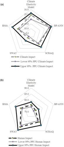
The BMA mean prediction of quantitative approaches and their individual outputs are shown in Table 6. The results indicate that the human activities have larger impacts on streamflow in the basin in all of the applied approaches; except TS09. Hydrological simulation approach showed the largest impact of human activities on streamflow (about 85%), while the BP-ANN approach showed the least impact of human activities (about 74%). Compared with the individual approach predictions in Ajichay basin, BMA mean prediction showed that climate variations and changes in human activities contributed, respectively, to about 19.6% and 79.0% changes in streamflow in the Akhola watershed and 19.7% and 79.6% in the Vanyar watershed. The results of 95% uncertainty intervals of each method, as well as BMA, for the climate and human impacts are shown in Fig. 11(a) and (b), respectively. Clearly, 95% uncertainty bands of the individual approaches have deviation ranges of between 5% and 25% for climate impact and between 64% and 90% for human impacts. However, the uncertainty interval of BMA mean prediction varies in the ranges 14–27% and 74–80%, respectively, for climate and human impacts. This interval is slightly wider than for the BP-ANN and SCRAQ data-driven approaches.

Table 6. Results of Bayesian model averaging and its four individual approaches in the separation of climate and human impacts on Ajichay basin streamflow.

Method	% Climate impact	% Human impact
Climate elasticity model	24.4	75.6
BP-ANN	26.2	73.8
SCRAQ	19.1	80.9
SWAT	10.9	85.1
BMA	19.7	79.1

Figure 11. Mean prediction and 95% confidence intervals of BMA and four individual approaches for: (a) climate impact and (b) human impact (PPU: percent prediction uncertainty; BMA: Bayesian model averaging; BP-ANN: back-propagation ANN; SCRAQ: slope change ratio of accumulative quantity; SWAT: Soil and Water Assessment Tool).

5 Discussion

5.1 Trend analysis of climatic variables and river flow

The Mann-Kendall trend test analysis showed a negative trend in streamflow, no trend in precipitation and positive trends in temperature and PET. The change point analysis of streamflow also revealed that 1996/97 is the change point of Ajichay streamflow. These findings are in agreement with those of Delju et al. (2013) and Fathian et al. (2015), whose studies focused on climatic and hydrological factors in the Lake Urmia basin, by analysing trends in precipitation, temperature and streamflow time series. It was shown that there was an increase in the temperature, while streamflow decreased significantly with a more intense reduction in downstream areas. Moreover, the trend in precipitation was not the same in all parts of the basin. However, they highlighted the need to study the impacts of human activities in addition to climate.

Furthermore, Fathian et al. (2016) studied the impacts of land-cover changes and climate variability in the eastern sub-basins of Lake Urmia (including Ajichay), in which greater sensitivity of streamflow to changes in land cover (as an anthropogenic impact) was verified.

5.2 Separating climatic and anthropogenic impacts

Evaluation of climatic and human impacts shows that all of the methods, except for TS09, identified human activities as the dominant impact on streamflow. As the TS09 method, as a climatological data-based method, does not divide the period into pre- and post-change periods and compares the relative change of P_ex and E_ex, it could have more uncertainties.

Quantitative assessment of human and climate impacts revealed that climate variations resulted in a decrease in river flow of 1.01–2.43 m³ s⁻¹ in the period 1987–2007 for the Ajichay basin. The effects of human activities on the river flow decrease were accountable for about 6.86–7.90 m³ s⁻¹, which amounts to 73.8–85.1% of the river flow changes.

Previous studies by other researchers have also shown the more significant impacts of human activities: Ghodousi (2012), using SWAT and taking a relatively different approach, found land-use change and dam operations as the main driving forces that changed the inflow to Lake Urmia. AghaKouchak et al. (2015) carried out a remote sensing analysis along with studying gauged climate data. Comparing the trends in droughts and the standardized precipitation index (SPI) with the change in area of the lake, they concluded that these changes are mainly due to human activities in the area. Jalili et al. (2016), comparing the changes in water level of the lake with the results obtained from analysis of the Southern Oscillation Index (SOI) and the North Atlantic Oscillation (NAO), showed that these latest reductions in water level of Lake Urmia are mainly due to human activities. Fazel et al. (2017) also indicated that irrigation was the dominant cause of changes in the flow regime of Lake Urmia. Chaudhari et al. (2018) applied a remote sensing analysis, ground observed data and the HiGW-MAT model (a hydrological modelling approach). They concluded that human activities were the greater contributor (86%) to the reduction in water level in the period 1995–2010. Moreover, Shadkam et al. (2016b), applying the variable infiltration capacity (VIC) model, analysed the lake under different climatic and anthropogenic scenarios for past and future periods and realized that anthropogenic scenarios could be significant drivers in the historical inflow to the lake.

Despite the increasing number of researchers stating that anthropogenic impacts are responsible for the desiccation of Lake Urmia, one study (Shadkam et al. 2016a) opines that about 60% of the change is due to climate variations. This difference could be because of the area or the period of time covered in their study. Meanwhile, in this study, the study chosen was the Ajichay River Basin, in which there have been significant anthropogenic changes, including the development of agricultural areas and irrigation networks, as well as the construction of multiple dams. Therefore, there might be different levels of land-use changes and human activities in various parts and catchments of Lake Urmia Basin which had led to its desiccation.

The human activities, e.g. increase in irrigated agricultural area, change in cropping patterns (land-use and land-cover changes) and, therefore, intensified water withdrawal, urbanization and river regulation, may be the main reasons for alterations in the Ajichay River flow since 1997. Among these, some anthropogenic impacts, such as increased water extraction, the effect of dam construction and/or operation and population growth, with consequent change in the domestic water demand, might be more linear and easier to detect.

5.3 Uncertainty analysis of the results

The between- and within-model uncertainty analyses of the applied techniques, using the combined Monte Carlo–BMA method, show that the 95% uncertainty intervals of both BMA and individual approaches have relatively large deviation ranges. The uncertainty interval of BMA mean prediction is a little broader than the black-box modelling approaches, but it can reduce the between-model uncertainties which vary in the ranges 14–27% and 74–80%, respectively, for climatic and human impacts. Major sources of uncertainties in the approaches used may arise from the model parameters and also input data.

It is found that, considering major sources of uncertainties in separating climatic and anthropogenic impacts on the streamflow, the BMA uncertainty interval could have a better performance than each individual approach. Moreover, the mean probabilistic prediction of different approaches generally leads to more realistic results than its individual model predictions. Therefore, considering uncertain results of competing methods available for this problem, the BMA between- and within-model uncertainty analysis is particularly a useful method to quantify the impacts of climate variations and anthropogenic activities on the river flow. The BMA uncertainty interval could consider the relative results of applied methods by assigning a certain weight to each method. Using weighted averaging of uncertain results of all methods could produce more accurate uncertainty interval and mean prediction.

5.4 Limitations of the multi-model ensemble approach

Two main issues in this study need to be pointed out. Regarding the driving forces affecting the streamflow, this study does not comprise trend analysis of the physical changes forced into the river flow (such as constructions of reservoir dams and water distribution networks, land-use and land-cover change, etc.). Therefore, in order to present realistic results with lower uncertainties, it is recommended to include such considerations and their interactions with hydrological changes.

Furthermore, this study was based on quantification of climatic and anthropogenic impacts on the streamflow and these two kinds of impacts were assessed separately. However, there are some interactions between climatic and anthropogenic impacts on the hydrology of a basin. These combined impacts of climate change and human activities (as presented by different studies, e.g. Wang et al. (2010), Zhang et al. (2012), etc.) could play an important role in some basins, especially those with high levels of climate variations. Hence, to further study the impacts of different driving forces and provide more accurate results, one could also take the combined effects of climatic and anthropogenic changes into consideration.

6 Conclusion

The aim of this paper was to address the uncertain impacts of human activities and climate variations on streamflow using different separation methods. To this end, a multi-model ensemble method based on the Monte Carlo-Bayesian model averaging (BMA) was used to combine and analyse the level of uncertainties of multiple results from both statistical and simulation-based methods. The applied techniques comprised: (i) statistical methods (TS09, climate elasticity model and SCRAQ), and (ii) simulation-based methods (BP-ANN and SWAT hydrological modelling). This study reported the application of the proposed approach regarding the Ajichay River Basin in Iran. This approach could help to better understand how the river flow responds to driving forces considering within- and between-model uncertainties of separation approaches. The main conclusions drawn from our study are as follows:

• Statistical methods are relatively easier to apply and are more flexible for separating the impacts of human activities and climate variations in poorly gauged basins. However, the level of between-model uncertainties is relatively high for these methods. As in this study, the results showed that the 95% uncertainty bands of the statistical approaches have deviation ranges of between 12% and 25% for climate impacts and between 64% and 80% for human impacts. These uncertainties mainly result from differences in various aspects that different methods take and their analytical structure. Moreover, simulation-based methods are more complex and are able to consider different components of interrelated systems. However, because of taking more parameters into account, the level of within-model uncertainties is higher than the former methods.

• There is a wide range of uncertainty in parameterizations of human impacts compared to climate impacts (about twice as high as climate impacts uncertainty), which is mainly due to the diversity of anthropogenic factors affecting the river flow. In this regard, conceptual simulation-based methods with consideration of different human-induced driving forces (e.g. reservoirs, land-use change and irrigation) provide more detailed outputs for better hydrological analysis. However, due to lack of data in poorly gauged regions, there are some limitations in the application of these models.

• Taking a wider range of separation methods and using a probabilistic multi-model ensemble approach provides better information than any of the individual methods. Therefore, that would be a helpful means for the realistic decision-making. The proposed BMA-based ensemble prediction methods in this study are promising approaches for reducing the uncertainty levels in separation of human and climate impacts on river flow.

Disclosure statement

No potential conflict of interest was reported by the authors.

Notes

¹ http://earthexplorer.usgs.gov.demexplorer.

Appendix

SWAT model set-up and calibration

In order to set up the model, different GIS layers, including the digital elevation model (DEM), soil type, and land use are required. The DEM layer of Ajichay River basin with a cell size of 30 m was provided for free by a USGS website.¹ The soil map and cropping pattern data were obtained from the Food and Agriculture Organization global soil map (FAO 1995), and the Iranian Ministry of Agriculture, respectively. Land-use layers used in this study (1989, 2002, and 2007) were interpreted from the Landsat5 TM dataset with a resolution of 30 m (Fathian 2012, Fathian et al. 2013). These were used to update land use in the model.

The hydrometric stations were used to divide the river basin into 36 sub-basins based on DEM and the stream network layers. Afterward, land-use, soil and slope layers were overlapped and subdivided sub-basins into 402 HRUs, among which 198 HRUs are irrigated agricultural lands. The management operation of wheat, barley, potato, tomato, sugar beet, alfalfa and apple, as seven major crops, was assigned to each HRU based on the average distribution of crops with no crop rotation.

In order to simulate irrigation practices, the “irrigation schedule by date” option was employed, instead of “auto irrigation” like many other studies in rural areas. Water demand for crops was prepared from Iran’s National Water Document (INWD) (Alizadeh and Kamali 2007) and sources of irrigation were defined based on the Comprehensive Water Management Plan (CWMP; Ministry of Energy 2006).

The daily precipitation and temperature data from 10 meteorological stations for the period 1987–2007 were collected from the Islamic Republic of Iran Meteorology Organization (IRIMO) and the Ministry of Energy.

The daily inflow, annual crop yield, and actual evapotranspiration data and the measured streamflow data for the baseline period were used to calibrate the model. The warm-up period was considered to be the first 2 years of the simulation periods to minimize the effect of initial default conditions (White et al. 2012). In order to eliminate the impacts of climatic variations, the climatic parameters were detrended. In this study, the SWAT-CUP model (Abbaspour et al. 2007) was utilized for the calibration and sensitivity analysis, applying 20 hydrological parameters, including soil, land use, reach, groundwater, surface runoff, and snow.

First, sensitivity analysis of the model was performed (Table A1) and found that SCS runoff curve number, soil evaporation compensation factor, and moist bulk density were the most sensitive parameters in changing the streamflow. While effective hydraulic conductivity in the main channel was obtained as the least sensitive parameter (Ghodousi 2012). For more information about the parameters, the reader is referred to the SWAT documents.

Then, daily observed data at the gauging stations were applied to calibrate and validate the model. In order to evaluate the streamflow simulations, two commonly used coefficients were applied. These coefficients are the coefficient of determination (R²) and Nash-Sutcliffe (NS) coefficient. Based on the results, the model assessment based on R² showed a range of 0.68 to 0.74 for the calibration period, while the corresponding values for the validation period were 0.54 to 0.69 (Table A2). In addition, the corresponding values for NS are 0.57 to 0.60 for the calibration period and 0.64 to 0.67 for the validation period.

Crop yield and AET were calibrated simultaneously, because of their mutual effects. Although this method involves a higher cost of computation and needs more time, as shown in the next sections, it yields more accurate and realistic results.

Sensitivity analysis of model parameters including Brown (maximum potential) Leaf Area Index (BLAI), minimum base temperature (T_base) for the plant growth (ºC), the optimal growing conditions harvest index (HVSTI), maximum LAI fraction at the first and second points on the optimal leaf area development curve (LAIMX1 and LAIMX2), fraction of plant growing season (FRGRW1) and second point fraction of plant growing (FRGRW2) was carried out by SWAT-CUP. In order to determine the optimal values of the above parameters, available information and the suggested parameters for the same crops in LU basin were used (Ahmadzadeh 2009).

It was evaluated how the simulated values for crop yield and AET were close to the regional data (MOA 2007) and crop water demands provided in Iran’s National Document of Water (INDW) for the study area (Alizadeh and Kamali 2007), respectively. AET was compared only for the wet years such as the year 2006 so that it could be assumed that no water stress existed. As the results show, the values for modelled AET were very close to the values for maximum crop water requirements (PET) reported by the INDW (AET = PET).

The final results for the crop yield and AET simulation are shown in Table 8. As can be seen, the estimated and recorded crop yields are similar such that for all crops R² is 0.99. The simulated monthly AET for 2006 by SWAT and the INDW reported values (Alizadeh and Kamali 2007), with R² =0.88, showed the acceptable performance of the model (Table A3).

Table A1. Sensitivity analysis of SWAT parameters. t: Student’s t statistic.

Rank	Parameter	Definition (SWAT input data)	t	p	Initial range	Final range
1	CN2	Initial SCS runoff curve number for moisture condition II	3.95	0	35–80	60–70
2	ESCO	Soil evaporation compensation factor	2.11	0.04	0.01–1	0.95–1
3	SOL–BD(1)	Moist bulk density (mg m^−3 or g cm^−3)	2.08	0.04	1.2–1.6	1.3–1.5
4	GWQMN	Threshold depth of water in the shallow aquifer required for return flow to occur (mm H2O)	1.93	0.06	100–3000	0–2
5	ALPHA_BNK	Baseflow alpha factor for bank storage (d)	1.09	0.28	0–1	0.4–0.6
6	CH_N(2)	Manning’s n for the main channel	0.92	0.36	0.01–0.3	0.013–0.016
7	ALPHA_BF	Baseflow alpha factor (day^−1)	0.84	0.41	0–1	0.1–0.4
8	GW_REVAP	Groundwater re-evaporation coefficient	0.79	0.44	0.02–0.2	0.02–0.025
9	SOL_K(1)	Saturated hydraulic conductivity (mm h^−1)	0.69	0.49	0.1–200	20–30
10	SOL_AWC(1)	Available water capacity of the soil layer (mm soil)	0.48	0.63	0.1–0.32	0.28–0.32
11	GW_DELAY	Groundwater delay time (days)	0.43	0.67	1–60	20–35
12	SFTMP	Snowfall temperature (°C)	0.24	0.81	(–5)–5	(–5)–5
13	CH_K(2)	Effective hydraulic conductivity in main channel (mm h^−1)	0.22	0.83	0.1–1000	20–50

Table A2. Model performance summary for calibration and validation periods.

Station	Calibration			Validation
	Period	R^2	NS	Period	R^2	NS
Akhola	1987–1999	0.74	0.57	2000–2007	0.69	0.67
Vanyar	1987–1999	0.68	0.60	2000–2007	0.54	0.64

R², coefficient of determination; NS, Nash-Sutcliffe efficiency.

Table A3. Observed and simulated yield and annual averages of simulated actual evapotranspiration (AET) for the major crops in the study area.

Parameter	Crop
	Wheat	Barley	Potato	Tomato	Sugar beet	Alfalfa	Apple
Mean reported yield (t ha^−1)	3.46	2.69	21.17	33.03	44.60	8.50	22.14
Mean simulated yield (t ha^−1)	3.49	2.41	23.00	36.00	43.80	9.83	24.22
Observed annual average AET (mm year^−1)	360	354	536	517	634	854	757
Simulated annual average AET (mm year^−1)	410	406	651	566	736	857	630

References

- Abbaspour, K.C., et al., 2007. SWAT-CUP calibration and uncertainty programs. A User Manual. Zurich, Switzerland: EAWAG.
- AghaKouchak, A., et al., 2015. Aral sea syndrome desiccates lake Urmia: call for action. Journal of Great Lakes Research, 41 (1), 307–311. doi:10.1016/j.jglr.2014.12.007
- Ahmadzadeh, H., 2009. Evaluation of agricultural water productivity using SWAT model. Case study: Zarinehrood basin. MSc. Thesis. Tarbiat Modares University, Iran.
- Ahn, K.H. and Merwade, V., 2014. Quantifying the relative impact of climate and human activities on streamflow. Journal of Hydrology, 515, 257–266. doi:10.1016/j.jhydrol.2014.04.062
- Ajami, N.K., et al., 2006. Multimodel combination techniques for analysis of hydrological simulations: application to distributed model intercomparison project results. Journal of Hydrometeorology, 7 (4), 755–768. doi:10.1175/JHM519.1
- Alizadeh, A. and Kamali, G.A., 2007. Crops water requirements. Mashhad, Iran: Imam Reza University Press.
- Bai, P., Liu, W., and Guo, M., 2014. Impacts of climate variability and human activities on decrease in streamflow in the Qinhe river, China. Theoretical and Applied Climatology, 117, 293–301. doi:10.1007/s00704-013-1009-7
- Breiman, L., 1996. Bagging predictors. Machine Learning, 24 (2), 123–140. doi:10.1007/BF00058655
- Chang, J., et al., 2014. Impact of climate change and human activities on runoff in the Weihe river basin, China. Quaternary International, xxx, 1–11. (in press).
- Chaudhari, S., et al., 2018. Climate and anthropogenic contributions to the desiccation of the second largest saline lake in the twentieth century. Journal of Hydrology, 560, 342–353. doi:10.1016/j.jhydrol.2018.03.034
- Chen, Z., Chen, Y., and Li, B., 2013. Quantifying the effects of climate variability and human activities on runoff for Kaidu river basin in arid region of northwest China. Theoretical and Applied Climatology, 111, 537–545. doi:10.1007/s00704-012-0680-4
- Cong, Z., et al., 2017. Attribution of runoff change in the alpine basin: a case study of the Heihe Upstream basin, China. Hydrological Sciences Journal, 62 (6), 1013–1028. doi:10.1080/02626667.2017.1283043
- Delju, A.H., et al., 2013. Observed climate variability and change in Urmia lake basin, Iran. Theoretical and Applied Climatology, 111 (1–2), 285–296. doi:10.1007/s00704-012-0651-9
- FAO (Food and Agriculture Organization), 1995. Digital soil map of the world. Version 3.5. [CD-ROM]. Food and Agriculture Organization of the United Nations.
- Fathian, F., 2012. Trend assessment of land use changes using remote sensing technique and hydro-climatological variables in Urmia lake basin. Master’s thesis. Tehran, Iran: Tarbiat Modares University. (In Persian).
- Fathian, F., Dehghan, Z., and Eslamian, S., 2016. Evaluating the impact of changes in land cover and climate variability on streamflow trends (case study: eastern subbasins of lake Urmia, Iran). International Journal of Hydrology Science and Technology, 6 (1), 1–26. doi:10.1504/IJHST.2016.073881
- Fathian, F., Morid, S., and Arshad, S., 2013. Trend assessment of land use changes using remote sensing technique and its relationship with streamflows trend (Case study: the East sub-basins of Urmia lake). Journal of Water and Soil, 27 (3), 642–655. (In Persian).
- Fathian, F., Morid, S., and Kahya, E., 2015. Identification of trends in hydrological and climatic variables in Urmia lake basin, Iran. Theoretical and Applied Climatology, 119 (3–4), 443–464. doi:10.1007/s00704-014-1120-4
- Fazel, N., Haghighi, A.T., and Kløve, B., 2017. Analysis of land use and climate change impacts by comparing river flow records for headwaters and lowland reaches. Global and Planetary Change, 158, 47–56. doi:10.1016/j.gloplacha.2017.09.014
- Fraley, C., et al., 2011. ensembleBMA: an R package for probabilistic weather forecasting. Massachusetts: American Meteorological Society.
- Gassman, P.W., et al., 2007. The soil and water assessment tool: historical development, applications, future research directions. Transactions of the American Society of Agricultural and Biological Engineers, 50 (4), 1211–1250.
- Ghodousi, M., 2012. Impact of rainfall patterns, land use changes and exploitation of Vanyar dam on hydrology of Ajichay basin and its impact on lake Urmia. Master’s thesis. Tarbiat Modares University, Tehran, Iran. (In Persian).
- Guo, Y., et al., 2014. Quantitative assessment of the impact of climate variability and human activities on runoff changes for the upper reaches of Weihe river. Stochastic and Environmental Research Risk Assessment, 28, 333–346. doi:10.1007/s00477-013-0752-8
- Hoeting, J.A., et al., 1999. Bayesian model averaging: a tutorial. Statistical Science, 14 (2), 382–401.
- Hu, Z., et al., 2015. Quantitative assessment of climate and human impacts on surface water resources in a typical semi-arid watershed in the middle reaches of the Yellow river from 1985 to 2006. International Journal of Climatology, 35, 97–113. doi:10.1002/joc.2015.35.issue-1
- Huang, S., et al., 2016. Contributions of climate variability and human activities to the variation of runoff in the Wei river basin, China. Hydrological Sciences Journal, 61 (6), 1026–1039. doi:10.1080/02626667.2014.959955
- Huang, S., Huang, Q., and Chen, Y., 2014. Quantitative estimation on contributions of climate changes and human activities to decreasing runoff in Weihe river basin, China. Chinese Geographical Science, 25 (5), 569–581.
- Jalili, S., Hamidi, S.A., and Namdar Ghanbari, R., 2016. Climate variability and anthropogenic effects on lake Urmia water level fluctuations, northwestern Iran. Hydrological Sciences Journal, 61 (10), 1759–1769.
- Kendall, M.G., 1975. Rank correlation methods. London, UK: Griffin.
- Khoi, D.N. and Suetsugi, T., 2014. Impact of climate and land-use changes on hydrological processes and sediment yield—a case study of the Be River catchment, Vietnam. Hydrological Sciences Journal, 59 (5), 1095–1108. doi:10.1080/02626667.2013.819433
- Li, Y., et al., 2016. Contributions of climate variability and human activities to runoff changes in the upper catchment of the red river basin, china. Water, 8 (9), 414.
- Liu, D., et al., 2010. Impacts of climate change and human activities on surface runoff in the Dongjiang river basin of China. Hydrological Processes, 24, 1487–1495. doi:10.1002/hyp.v24:11
- Ma, F., et al., 2014. An estimate of human and natural contributions to flood changes of the Huai river. Global and Planetary Change, 119, 39–50. doi:10.1016/j.gloplacha.2014.05.003
- Mann, H.B., 1945. Nonparametric tests against trend. Econometrica: Journal of the Econometric Society, 13, 245–259. doi:10.2307/1907187
- Metropolis, N. and Ulam, S., 1949. The monte carlo method. Journal of the American Statistical Association, 44 (247), 335–341. doi:10.1080/01621459.1949.10483310
- Ministry of Energy, 2006. Comprehensive water management plan. Tehran, Iran: Ministry of Energy (In Persian).
- MOA (Ministry of Agriculture), 2007. Agricultural statistics and the information center. Tehran, Iran: Iranian Ministry of Jahade-Agriculture.
- Moon, T.K., 1996. The expectation-maximization algorithm. IEEE Signal Processing Magazine, 13 (6), 47–60. doi:10.1109/79.543975
- Niraula, R., Meixner, T., and Norman, L.M., 2015. Determining the importance of model calibration for forecasting absolute/relative changes in streamflow from LULC and climate changes. Journal of Hydrology, 522, 439–451. doi:10.1016/j.jhydrol.2015.01.007
- Pettitt, A.N., 1979. A non-parametric approach to the change-point problem. Applied Statistics, 28, 126–135. doi:10.2307/2346729
- Raeisi, A.A., Bijani, M., and Chizari, M., 2018. The mediating role of environmental emotions in transition from knowledge to sustainable behavior toward exploit groundwater resources in Iran’s agriculture. International Journal of Soil Water Conservation Research, 6 (2), 143–152. doi:10.1016/j.iswcr.2018.01.002
- Renner, M., Seppelt, R., and Bernhofer, C., 2012. Evaluation of water-energy balance frameworks to predict the sensitivity of streamflow to climate change. Hydrology and Earth System Sciences, 16 (5), 1419–1433.
- Schapire, R.E., 1990. The strength of weak learnability. Machine Learning, 5 (2), 197–227. doi:10.1007/BF00116037
- Shadkam, S., et al., 2016a. Impacts of climate change and water resources development on the declining inflow into Iran’s Urmia lake. Journal of Great Lakes Research, 42 (5), 942–952. doi:10.1016/j.jglr.2016.07.033
- Shadkam, S., et al., 2016b. Preserving the world second largest hypersaline lake under future irrigation and climate change. Science of the Total Environment, 559, 317–325. doi:10.1016/j.scitotenv.2016.03.190
- Tan, M.L., et al., 2015. Impacts of land-use and climate variability on hydrological components in the Johor river basin, Malaysia. Hydrological Sciences Journal, 60 (5), 873–889.
- Tang, J., et al., 2014. Assessment of contributions of climatic variation and human activities to streamflow changes in the Lancang river, China. Water Resources Management, 28, 2953–2966. doi:10.1007/s11269-014-0648-5
- Thornthwaite, C.W., 1948. An approach toward a rational classification of climate. Geographical Review, 38 (1), 55–94. doi:10.2307/210739
- Tomer, M. and Schilling, K.E., 2009. Discerning climate and land-use change impacts on watershed hydrology: implications for Gulf Hypoxia. Meeting Abstract, 51.
- Valiant, L.G., 1984. A theory of the learnable. In: Proceedings of the sixteenth annual ACM symposium on theory of computing, December, Washington, DC. ACM, 436–445.
- Wang, J., et al., 2010. Quantitative assessment of climate change and human impacts on long‐term hydrologic response: a case study in a sub‐basin of the Yellow river, China. International Journal of Climatology, 30 (14), 2130–2137. doi:10.1002/joc.v30:14
- Wang, S., et al., 2012a. Contributions of climate change and human activities to the changes in runoff increment in different sections of the Yellow river. Quaternary International, 282, 66–77. doi:10.1016/j.quaint.2012.07.011
- Wang, S., et al., 2012b. Quantitative estimation of the impact of precipitation and human activities on runoff change of the Huangfuchuan river Basin. Journal of Geographical Science, 22 (5), 906–918. doi:10.1007/s11442-012-0972-8
- Wang, S., et al., 2013. Isolating the impacts of climate change and land use change on decadal streamflow variation: assessing three complementary approaches. Journal of Hydrology, 507, 63–74. doi:10.1016/j.jhydrol.2013.10.018
- Wang, S., et al., 2015. Climatic and anthropogenic impacts on runoff changes in the Songhua river basin over the last 56 years (1955–2010), Northeastern China. Catena, 127, 258–269. doi:10.1016/j.catena.2015.01.004
- Wang, X., 2014. Advances in separating effects of climate variability and human activity on stream discharge: an overview. Advances in Water Resources, 71, 209–218. doi:10.1016/j.advwatres.2014.06.007
- White, M.J., et al., 2012. SWAT check: a screening tool to assist users in the identification of potential model application problems. Journal of Environmental Quality, 43 (1), 208–214. doi:10.2134/jeq2012.0039
- Xia, J., et al., 2014. Quantifying the effects of climate change and human activities on runoff in the water source area of Beijing, China. Hydrological Sciences Journal, 59 (10), 1794–1807. doi:10.1080/02626667.2014.952237
- Ye, X., et al., 2013. Distinguishing the relative impacts of climate change and human activities on variation of streamflow in the Poyang lake catchment, China. Journal of Hydrology, 494, 83–95. doi:10.1016/j.jhydrol.2013.04.036
- Zhang, A., et al., 2012. Assessments of impacts of climate change and human activities on runoff with SWAT for the Huifa river Basin, Northeast China. Water Resources Management, 26, 2199–2217. doi:10.1007/s11269-012-0010-8
- Zhang, L., Dawes, W.R., and Walker, G.R., 2001. Response of mean annual evapotranspiration to vegetation changes at catchment scale. Water Resources Research, 37 (3), 701–708. doi:10.1029/2000WR900325
- Zhao, C., et al., 2015. Separation of the impacts of climate change and human activity on runoff variations. Hydrological Sciences Journal, 60 (2), 234–246. doi:10.1080/02626667.2013.865029
- Zhao, F., et al., 2010. Evaluation of methods for estimating the effects of vegetation change and climate variability on streamflow. Water Resources Research, 46, 3. doi:10.1029/2009-WR007702