Water quality monitoring at a virtual watershed monitoring station using a modified deep extreme learning machine

ABSTRACT

A new deep extreme learning machine (ELM) model is developed to predict water temperature and conductivity at a virtual monitoring station. Based on previous research, a modified ELM auto-encoder is developed to extract more robust invariance among the water quality data. A weighted ELM that takes seasonal variation as the basis of weighting is used to predict the actual value of water quality parameters at sites which only have historical data and no longer generate new data. The performance of the proposed model is validated against the monthly data from eight monitoring stations on the Zengwen River, Taiwan (2002–2017). Based on root mean square error, mean absolute error, mean absolute percentage error and correlation coefficient, the experimental results show that the new model is better than the other classical spatial interpolation methods.

KEYWORDS:

• weighted extreme learning machine
• contractive denoising auto-encoder
• virtual monitoring station
• water quality prediction

Editor S. Archfield Associate editor Xun Sun

1 Introduction

Water bodies should be monitored at a spatial scale that provides information on their current state and highlights where new management actions may be needed, or if current management practices are sufficient (Reyjol et al. 2014). Hence, the greater the number of monitoring sites throughout a water body, the higher the probability that monitoring will accurately represent its current state. However, according to market research conducted by the author, in China, the construction cost of a small automatic monitoring station with five water quality parameters (permanganate index, ammonia nitrogen, total phosphorus, water temperature, pH) is up to 4 million RMB, which does not include the subsequent equipment maintenance and human resources. Therefore, there are resource implications where a large number of monitoring sites are required and a balance is needed between resource requirements and scientific rigor (Earle and Blacklocke 2008).

In the early 20th century, Prandtl (1925) proposed and developed the mixing length theory that describes mixing length as the distance over which a fluid parcel will maintain its properties before it is mixed with the surrounding fluid. In other words, river mixing length is a distance over which an upstream water parcel will keep its original properties before dispersing those characteristics into the surrounding downstream water (Do et al. 2012). Therefore, in order to reduce maintenance costs, it is possible to optimize the built monitoring network based on this theory (Chapman et al. 2016). For this reason, many researchers have studied methods that are mostly based on statistical theory (Guigues et al. 2013, Mavukkandy et al. 2014, Wang et al. 2014, Tanos et al. 2015, Villas-Boas et al. 2017), the kriging method (Karamouz et al. 2009a, Chunping et al. 2012, Sabzipour et al. 2017), or information entropy (Karamouz et al. 2009b, Lee et al. 2014). For instance, Maymandi et al. (2018) proposed a hybrid VOI-entropy-based methodology to optimize a water quality monitoring network built on the largest manmade reservoir in Iran. In order to optimize the monitoring network in the Taizihe River, Northeast China, the matter element analysis and gravity distance were applied in the optimization, which was proved to be a useful method (Wang et al. 2015). Furthermore, they found that the number of monitoring stations in the network could be reduced from 17 to 13. Antanasijević et al. (2017) proposed a self-organizing network based on the similarity index for the optimization of sampling locations in an existing river water quality monitoring network of the River Danube on its stretch through Serbia. The study by Chapman et al. (2016) used combined cluster and discriminant analysis (Kovács et al. 2014) to evaluate the efficiency of a monitoring network in the Danube River.

After optimization through the methods described above, some sites in a monitoring network can be closed and monitoring can be stopped to reduce subsequent maintenance costs. Such monitoring stations that only have historical data and no longer generate new data, are referred to as ‘virtual stations’ in this paper. Although the trend of change can be inferred from contiguous sites with high correlation, the specific values cannot be known. For example, when a new source of pollution appears near the optimized monitoring station, it is necessary to obtain specific values of pollutants at the current monitoring points to judge the severity of the pollution (Mitrović et al. 2019). Appropriate methods, such as ordinary kriging (OK) and inverse distance weighting (IDW) (Mehrjardi et al. 2008, Yang and Jin 2010) are developed to interpolate the inactive sites and infer water quality conditions at unmonitored sites. Recently, Rizo-Decelis et al. (2017) adapted an improved topological kriging (TK) method to estimate water quality along the main stem of a large basin. Based on cross-validation experiments applied to 28 water quality variables measured along the Santiago River in western Mexico, they showed that the TK method offers a more accurate water quality prediction than other methods (including OK) for many of the measured parameters. Laaha et al. (2013) employed the TK method and regional regression to estimate streamflow-related variables along streams in Austria and found that the TK method is well suited for streamflow and many streamflow-related variables. Jiang et al. (2013) use the OK method to predict the spatial distribution of various water quality parameters (salinity, pH, total hardness) in the Huaihe River basin, China.

With the development of artificial intelligence technology, the artificial neural network (ANN) has been proved to be superior to both the kriging method and partial thin-plate splines due to its strong fitting ability to non-linear systems (Juan 2003); and it has been successfully applied to various spatial interpolation tasks (Li et al. 2004, Philippopoulos and Deligiorgi 2012, Shahabi et al. 2016). In terms of the interpolation of the spatial distribution of water quality, Yingchun et al. (2013) proposed a model to spatially predict dissolved organic carbon (DOC) using an ANN and demonstrated that the ANN is a promising tool for the spatial prediction of DOC in river networks using watershed characteristics. Li et al. (2013) applied the model of genetic algorithm optimized back-propagation neural networks (GA-BPNN) to formulate the forecasting methodology of groundwater quality parameters, with spatial data as parameters. Compared with the OK method, the results of the GA-BPNN were better and the proposed method was found to be a reasonable and feasible method for the spatial distribution of groundwater quality parameters in Langfang city (China). In a study by Khashei-Siuki and Sarbazi (2015), IDW, kriging, cokriging, ANN and adaptive network-based fuzzy inference system (ANFIS) models were compared in the prediction of the spatial distribution of groundwater electrical conductivity (EC). Their results showed that the ANN model had the best accuracy. Mitrović et al. (2019) used a Monte Carlo optimized ANN to predict 18 water quality parameters at monitoring stations in the Danube River that had stopped operation since 2012. Their research showed that most of the studied water quality parameters (13 of 18) were estimated with smaller relative error (less than 10%), which means that it is reasonable for these monitoring stations to be optimized and disabled.

The traditional ANN often uses a back-propagation (BP) algorithm to train the model. Research shows that the BP algorithm is slow in learning, easy to fall into local optimum, and difficult to adapt to some real-time scenarios (Sotiropoulos et al. 2002). To solve these problems, Huang et al. (2006) proposed a new neural network model, the extreme learning machine (ELM). With the increasing complexity of a system, a shallow model with a simple structure has some limitations in problem analysis. For this reason, many researchers have improved the model based on ELM and developed deep models, such as the multi-layer ELM (Kasun et al. 2013), the denoising multi-layer ELM (Zhang et al. 2016) and the contractive multi-layer ELM (Jia and Du 2016), to realize automatic feature extraction. Based on these models, a new model that combines ELM with a contractive denoising auto-encoder (CDAE) is proposed in this paper, and the improved model is applied to predict the water quality at virtual stations in Zengwen River Basin, Taiwan.

Compared with the existing related methods of predicting the spatial distribution of water quality, the contributions of this paper are summarized as follows:

• local denoising criteria and a contractive regularization term are introduced simultaneously into the auto-encoder based on the ELM, and a deep contractive denoising ELM model is developed; and

• the proposed model is used to extract the abstract feature expression of the spatial water quality distribution relationship in the monitoring network, and the prediction of water quality at virtual stations is realized by the weighted extreme learning machine (WELM), which takes seasonal variation as the basis of weighting in the model.

The rest of the paper is organized as follows: Section 2 introduces the concepts of WELM, the auto-encoder and describes the proposed method. In Section 3, the Pearson correlation coefficient is used to analyse the spatial correlation of water temperature and conductivity collected from eight water quality monitoring stations near Zengwun River in Taiwan since 22 January 2002. Then, five algorithms including classical shallow models, i.e. the back propagation neural network (BPNN), ELM, WELM, deep ELM models, i.e. denoising multi-layer ELM, the proposed method, are used to predict actual values at the virtual monitoring sites through the observed values of relevant stations. Comparison of the prediction results is done using four indicators, i.e. RMSE, MAE, MAPE, R, to test the prediction performance of the proposed method. Finally, conclusions and future work are summarized.

2 Method

2.1 Weighted extreme learning machine (WELM)

The ELM is a learning method for training single hidden layer feedforward networks (SLFNs) and demonstrates its excellent learning accuracy and speed in a variety of applications (Huang et al. 2012). Suppose N training samples $\left[{\mathit{x}}_i,{\mathit{t}}_i\right],i=1,2,\dots ,N$, where each sample is denoted by ${\mathit{x}}_i=[x_{i1},x_{i2},\cdots ,x_{i{d}_x}{]}^T\in {\mathit{R}}^{d_x}$ and its corresponding network target vector is ${\mathit{t}}_i=[t_{i1},t_{i2},\cdots ,t_{i{d}_t}{]}^T\in {\mathit{R}}^{d_t}$, where $d_x$ and $d_t$ represent the dimensions corresponding to the input and output, respectively. Standard SLFNs with $l$ hidden nodes and activation function $g\left(x\right)$ are mathematically modelled as:

(1) ${\sum }_{j=1}^l{b}_j{g}_j\left({\mathit{x}}_i\right)={\sum }_{j=1}^l{b}_{j}g\left({\mathit{a}}_j{\mathit{x}}_i+b_j\right)={\mathit{t}}_i,i=1,2,\cdots ,N$(1)

where ${\mathit{a}}_j=\left(a_{j1},a_{j2},\cdots ,a_{j{d}_x}\right)$ is the weight vector connecting the jth hidden node and the input nodes; $b_j=\left(b_{j1},b_{j2},\cdots ,b_{j{d}_t}\right)$ is the weight vector connecting the jth hidden node and the output nodes; and $b_j$ represents the threshold of the jth hidden node.

The above equations may be written as:

(2) $\mathit{H}b=\mathit{T}$(2)

and the output weight $b$ can be calculated as:

(3) $b={\mathit{H}}^{†}\mathit{T}$(3)

where $\mathit{H}$ is the hidden layer node output matrix and expressed by Equation (4); $b=[b_1^T,b_2^T,\dots ,b_l^T{]}_{l\times d_t}^T$ is the output weight matrix; and $\mathit{T}=[t_1,t_2,\dots ,t_N{]}_{N\times d_t}^T$ is the expected output matrix.

(4) $\mathit{H}\left({\mathit{a}}_1,\dots ,{\mathit{a}}_l,b_1,\dots ,b_l,{\mathit{x}}_1,\dots {\mathit{x}}_N\right)={\left[\begin{array}{ccc}g\left({\mathit{a}}_1{\mathit{x}}_1+b_1\right)& \cdots & g\left({\mathit{a}}_l{\mathit{x}}_1+b_l\right)\\ ⋮& \ddots & ⋮\\ g\left({\mathit{a}}_1{\mathit{x}}_N+b_1\right)& \cdots & g\left({\mathit{a}}_l{\mathit{x}}_N+b_l\right)\end{array}\right]}_{N\times l}$(4)

In order to improve the robustness of the ELM, Deng et al. (2010) proposed a regularized ELM (RELM), which combines experiential risk with structural risk; the cost function can be rewritten as follows:

(5) $\underset{b}{\mathrm{m}\mathrm{i}\mathrm{n}}{L}_1=\frac{1}{2}\parallel b{\parallel }^2+\frac{C}{2}\parallel \mathit{T}-\mathit{H}b{\parallel }^2$(5)

where C is a regularization parameter to balance experiential risk and structural risk. The output weight $b$ can be expressed as:

(6) $b={\mathit{H}}^{†}\mathit{T}={\left(\frac{I}{C}+\mathit{H}{\mathit{H}}^T\right)}^{-1}{\mathit{H}}^T\mathit{T}$(6)

where ${\mathit{H}}^{†}$ is the Moore–Penrose generalized inverse of a matrix $\mathit{H}$.

Data in real applications such as water quality forecasting usually have imbalanced class distribution, which means some of the data in the time series are more important than others. To tackle the regression or classification tasks with imbalanced class distribution, the weighted ELM (WELM) is proposed by Zong et al. (2013).

The objective function of the WELM approach can be mathematically rewritten as:

(7a) $\mathrm{M}\mathrm{i}\mathrm{n}\mathrm{i}\mathrm{m}\mathrm{i}\mathrm{z}\mathrm{e}:L_{P_{\mathrm{E}\mathrm{L}\mathrm{M}}}=\frac{1}{2}\parallel b{\parallel }^2+\frac{1}{2}C{\sum }_{i=1}^N\mathit{W}{{\epsilon }_i}^2$(7a)

subject to:

(7b) $\mathit{h}\left({\mathit{x}}_i\right)b={\mathit{t}}_i-{\epsilon }_i,i=1,2,\dots ,N$(7b)

where ${\mathit{\epsilon }}_i=\left({\epsilon }_{i1},\epsilon i_2,\dots ,{\epsilon }_{i{d}_t}\right)$ is the training error of output $d_t$ corresponding to each input ${\mathit{x}}_i$; $\mathit{h}\left({\mathit{x}}_i\right)$ is the hidden layer node output vector of input ${\mathit{x}}_i$; and W is an $N\times N$ diagonal matrix with the diagonal element $w_{ii},i=1,2,\dots ,N$. In this paper, the weight matrix W is obtained by calculating the percentage of the sample size in the current quarter as a percentage of the total sample. Finally, according to the KKT (Karush-Kuhn-Tucker) theorem, the output weight matrix $b$ is given by:

(8) $b={\mathit{H}}^T(\frac{I}{C}+\mathit{W}\mathit{H}{\mathit{H}}^T{)}^{-1}\mathit{W}T$(8)

2.2 Auto-encoder

The Auto-encoder is a special neural network, which learns the input features in an unsupervised way and sets the target values to be equal to the input (Vincent et al. 2010). The auto-encoder is composed of an input layer, a hidden layer, and output layer. The structure of a basic auto-encoder is shown in Fig. 1.

Figure 1. Structure of the basic auto-encoder.

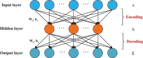
The auto-encoder consists of two processes, encoding and decoding. In the encoding phase, an encoding mapping $f$ that transforms the input vector $\mathit{x}\in {\mathit{R}}^{d_x}$ into a hidden representation $h\in {\mathit{R}}^{d_h}$:

(9) $h=f\left(\mathit{x}\right)=\mathrm{f}\mathrm{u}\mathrm{n}{\mathrm{c}}_f\left({\mathit{W}}_{1}x+b_1\right)$(9)

where $\mathrm{f}\mathrm{u}\mathrm{n}{\mathrm{c}}_f$ is the encoder activation function, which is usually a nonlinear function such as a sigmoid function or a hyperbolic tangent function. The matrix ${\mathit{W}}_1\in R^{d_h\times d_x}$ is the encoder weight, and $b_1\in R^{d_h}$ is the encoder bias. The parameters $d_x$ and $d_h$ represent the number of units in the input layer and hidden layer, respectively.

In the phase of the decoder network, the hidden representation $h$ is mapped back to a reconstruction $\tilde{x}\in R^{d_x}$ by the reconstruction function $\mathrm{f}\mathrm{u}\mathrm{n}{\mathrm{c}}_g$:

(10) $\tilde{x}=g\left(h\right)=\mathrm{f}\mathrm{u}\mathrm{n}{\mathrm{c}}_g\left({\mathit{W}}_{2}h+b_2\right)$(10)

where $\mathrm{f}\mathrm{u}\mathrm{n}{\mathrm{c}}_g$ is the decoder activation function, similar to $\mathrm{f}\mathrm{u}\mathrm{n}{\mathrm{c}}_f$. The decoder weight matrix is ${\mathit{W}}_2\in R^{d_x\times d_h}$ and the bias is $b_2\in R^{d_x}$. Generally, ${\mathit{W}}_2$ is equal to ${\mathit{W}}_1^T$ in practice. In this paper, ${\mathit{W}}_2={{\mathit{W}}_1}^T$. All parameters $\theta =\left\{W_1,W_2,b_1,b_2\right\}$ are learned simultaneously during the process of reconstruction and are as similar as possible to the original water quality data. This means that the loss function that can be expressed by Equation (11) needs to be minimized.

(11) $L\left(\theta \right)=\sum _{x\in X}D\left(x,\tilde{x}\right)+\frac{1}{2}\lambda \parallel W{\parallel }_2^2$(11)

where $X=\left\{x_1,x_2,\dots ,x_N\right\}$ is the training set with N samples; and $D$ is the reconstruction error, which can be mean square variance $D\left(x,\tilde{x}\right)=\frac{1}{n}{\sum }_{i=1}^n\frac{1}{2}\parallel {\tilde{x}}_i-{x_i}^2\parallel$. In order to avoid overfitting, the regularization term is added as the second part. The parameter $\lambda$ is a weight decay coefficient that controls the importance of the regularization.

For the purpose of learning robust representations, the denoising auto-encoder (DAE) (Vincent et al. 2010) and the contractive auto-encoder (CAE) are proposed (Rifai et al. 2011). The DAE is trained to reconstruct a clean “repaired” input from a corrupted version of it and the CAE with different regularization term can be described as follows:

(12) $L_{\mathrm{C}\mathrm{A}\mathrm{E}}\left(\theta \right)={\sum }_{x\in X}D\left(x,\tilde{x}\right)+\frac{1}{2}\lambda \parallel J\left(x\right){\parallel }_F^2$(12)

where $J\left(x\right)=\frac{\mathrm{\partial }f}{\mathrm{\partial }x}$ is the Jacobian matrix of the encoder $f$ at $x$. For a sigmoid encoder, the Frobenius norm $\parallel J\left(x\right){\parallel }_F^2$ can be calculated by (Liu et al. 2015):

(13) $\parallel J\left(x\right){\parallel }_F^2=\sum _{j=1}^{d_h}(f(x{)}_j(1-f\left(x{)}_j\right){)}^2{W_j}^2$(13)

2.3 Deep extreme learning machine based on ELM-CDAE

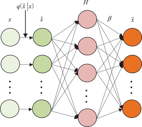
First, a new ELM model based on contractive denoising auto-encoder (ELM-CDAE) is presented; the model structure is shown in Fig. 2. The ELM-CDAE introduces the denoising criterion and regularization term in a contractive auto-encoder to guarantee that learning features are robust and useful.

Figure 2. Structure of the ELM-CDAE.

The original input $x$ is corrupted into $\hat{x}$ by means of a stochastic mapping $\hat{x}\to q\left(\hat{x}|x\right)$, and the cost function after adding the regularization term can be expressed as:

(14) $\underset{\beta }{\mathrm{m}\mathrm{i}\mathrm{n}}L=\frac{1}{2}\parallel \beta {\parallel }^2+\frac{C}{2}\parallel \mathit{T}-\mathit{H}\mathit{\beta }{\parallel }^2+\frac{\lambda }{2}\parallel J\left(x\right){\parallel }^2$(14)

Using the same method of computing as Equation (5), the output weights $\mathit{\beta }$ of ELM-CDAE can be computed as (Jia and Du 2016):

(15) $\mathit{\beta }={\left(\frac{I}{C}+\mathit{H}{\mathit{H}}^T+\lambda \frac{\mathrm{\partial }H}{\mathrm{\partial }x}\right)}^{-1}{\mathit{H}}^{T}X$(15)

The ELM-CDAE training algorithm is summarized as follows:

Step 1. Make use of the corrupting noise to corrupt initial samples $x$ and obtain corrupted samples $\hat{x}$. The noise can typically be Gaussian noise, Masking noise, Salt-and-pepper noise.

Step 2. Initiate the ELM-CDAE network with a given number of hidden nodes, randomly generate input weights matrix and biases, and then use corrupted samples $\hat{x}$ and Equation (4) to calculate the hidden layer output matrix $\mathit{H}$.

Step 3. Calculate the output weight matrix $\mathit{\beta }$ by Equation (15).

Then, a deep model based on ELM-CDAE and WELM is proposed. The model framework is shown in Fig. 3. Resembling the multi-layer ELM, which stacked the ELM auto-encoder (ELM-AE) (Kasun et al. 2013), the ELM-CDAE is stacked in this paper to create a new deep ELM model. Furthermore, the output of the connections between the last hidden layer and the output node is analytically calculated using the WELM approach.

Figure 3. Structure of the proposed model (ELM-CDAE).

Similar to the multi-layer ELM, each hidden layer in the deep ELM is trained in a bottom-up and greedy layer-wise manner. The raw input vectors, after being corrupted, are fed to the bottom auto-encoder. After training the bottom auto-encoder, the output hidden representations are wired to the subsequent layer. The same procedure is repeated until all the auto-encoders are trained. After this pre-training stage, the output is further fed into a WELM and the output weight is computed by Equation (8). Thus, the training of the whole network is completed.

The overall training procedure of the proposed model can be summarized as follows:

Step 1. Initiate the model parameters, including the number of hidden layers m, the number of each hidden unit, the input weights and biases. Select the activation function $g\left(x\right)$ and the corrupting noise.

Step 2. Pre-training stage:

For iteration m = 0:

(a) Make use of the corrupting noise to corrupt initial inputs $X$ and obtain corrupted inputs $\hat{X}$;

(b) Use all samples in $\hat{X}$ to train the ELM-CDAE and calculate the current layer output weight matrix ${\beta }_i$ by Equation (15).

Step 3. Calculate the output of the stacked ELM-CDAE:

(16) $f_{\mathrm{S}\mathrm{E}\mathrm{L}\mathrm{M}-\mathrm{C}\mathrm{D}\mathrm{A}\mathrm{E}}\left(x\right)={\beta }_m(g\left({\beta }_{m-1}\left(\dots g\left({\beta }_{0}x\right)\right)\right)$(16)

Step 4. Use the output of the stacked ELM-CDAE to calculate the weight matrix $\mathit{W}$ in the WELM by Laplacian regularized least squares method.

Step 5. Calculate the output weight matrix $\mathit{\beta }$ by Equation (15).

3 Experiments

3.1 Data description

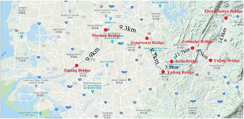
Monthly water quality data from eight water quality monitoring station near the Zengwun River, Taiwan, were collected between 22 January 2002 and 5 December 2017. These data are from the Taiwan Environmental Protection Agency¹. Figure 4 shows the distribution of the water quality monitoring stations and the symmetrical river network distance between two adjacent monitoring stations, which finds the shortest distance between two monitoring stations along the stream network.

Figure 4. Distribution of the water quality monitoring stations in the study area.

3.2 Performance metrics and settings

To evaluate the validity of the model, some sites with historical data are used as virtual sites, and the sites upstream and downstream of them are used as reference sites to predict the actual value of the virtual sites. The input of the proposed model is the observed water quality data of the reference sites at the current time, and the output is the predicted value of the virtual site at the current time. If the predicted results of the virtual site can show the real water quality of the virtual site more accurately, then the virtual site can be optimized in the monitoring network.

In the experiments, 70% of the data collected at each site are used as a training set for the basic models, and the remaining 30% is used as a test set to test the effectiveness of the models. The datasets need to be normalized before they can be used. Normalization is the scaling of data to a small-specific interval in order to remove the unit limit of the data and convert it to a pure dimensionless value. In this way, we can compare and give weights to different units or orders of magnitude. The normalized method used in this paper can be expressed as follows:

(17) ${\hat{x}}_i=\frac{x_i-x_{\mathrm{m}\mathrm{i}\mathrm{n}}}{x_{\mathrm{m}\mathrm{a}\mathrm{x}}-x_{\mathrm{m}\mathrm{i}\mathrm{n}}}$(17)

where ${\hat{x}}_i$ is the normalized value; and $x_i,x_{\mathrm{m}\mathrm{a}\mathrm{x}}$and $x_{\mathrm{m}\mathrm{i}\mathrm{n}}$ represent the sample, maximum and minimum values in the sample, respectively.

To evaluate the model, three statistical indices, RMSE, MAE and MAPE, and the correlation coefficient R, are used. These indicators can be formulated as follows:

(18) $\mathrm{R}\mathrm{M}\mathrm{S}\mathrm{E}=\sqrt{\frac{1}{N}{\sum }_{i=1}^N{({\hat{y}}_i-y_i)}^2}$(18)

(19) $\mathrm{M}\mathrm{A}\mathrm{E}=\frac{1}{N}{\sum }_{i=1}^N\left|{\hat{y}}_i-y_i\right|$(19)

(20) $\mathrm{M}\mathrm{A}\mathrm{P}\mathrm{E}=\frac{1}{N}{\sum }_{i=1}^N\frac{\left|{\hat{y}}_i-y_i\right|}{y_i}$(20)

(21) $R=\frac{{\sum }_{i=1}^N\left(y_i-\bar{y}\right)\left({\hat{y}}_i-\overline{\stackrel{ˆ}{y}}\right)}{\sqrt{{\sum }_{i=1}^N{(y_i-\bar{y})}^2{({\hat{y}}_i-\overline{\stackrel{ˆ}{y}})}^2}}$(21)

where $y_i,{\hat{y}}_i$and N are, respectively, the observed water quality parameter value, the predicted water quality parameter value and the number of test samples; and $\bar{y}$ and $\overline{\stackrel{ˆ}{y}}$ denote the observed and estimated means, respectively.

In addition, three classical shallow neural networks, the BPNN, ELM and WELM, and a deep ELM model based on ELM-DAE are used to verify the effectiveness of the proposed model. Furthermore, one mathematical method, OK, is also included. Some settings of these models are described as follow. The maximum number of iterations for the BPNN is 100. The Levenberg-Marquardt algorithm is adopted in the BPNN model. The activation function of the BPNN and ELM is a sigmoid function. The number of hidden nodes is gradually increased by an interval of 3 and the nearly optimal number of nodes for the BPNN and ELM are then selected based on threefold cross-validation method. The regularization parameter C for different datasets in the ELM and WELM models is to select the most suitable value from $\left[{10}^{-20},{10}^{-19},\dots ,{10}^{19},{10}^{20}\right]$ by cross-validation method. For the deep ELM model based on ELM-DAE, the number of neurons in each hidden layer is the same. The optimal number of hidden layers and neurons in each hidden layer can be obtained by the cross-validation method. For the regularization parameter $\lambda$ in the proposed model, the best parameters to deal with different datasets were found from a total of 100 values in the range 0–1 by setting an increment of 0.01. The parameters are described in detail in a later section. The semi-variogram function in the OK method can be expressed as follows:

(22) $\gamma \left(h\right)=c_0+c\left[1-exp\left(-\frac{h}{a}\right)cos\left(\frac{2\pi h}{b}\right)\right]$(22)

where $c_0,c,a$ and b are the parameters to be fitted and h is the distance between monitoring stations.

3.3 Spatial correlation analysis

The Pearson correlation coefficient can express the correlation of two variables, and its formula can be described as follows:

(23) ${\rho }_{X,Y}=\frac{{\sum }_{i=1}^N\left(X_i-\bar{X}\right)\left(Y_i-\bar{Y}\right)}{\sqrt{{\sum }_{i=1}^N{(X_i-\bar{X})}^2}\sqrt{{\sum }_{i=1}^N{(Y_i-\bar{Y})}^2}}$(23)

In order to analyse the spatial correlation of the water quality parameters, the Pearson correlation coefficient is used in this paper for selected monitoring stations; the results for water temperature and electrical conductivity are shown in Table 1, where the stations #1–#8 are numbered from upstream to downstream according to the real distribution of stations in the basin. For example, #1 is the First Zengwen Bridge station and #2 is Yujing Bridge station and so on.

Table 1. Correlation coefficient of water temperature and electrical conductivity between different stations. #1 is the First Zengwen Bridge station and #8 is Xigang Bridge station (see Fig. 4).

	#1	#2	#3	#4	#5	#6	#7	#8
Water temperature
#1	1	0.94673	0.95345	0.93992	0.88314	0.89111	0.91767	0.91500
#2	0.94673	1	0.96696	0.96280	0.91350	0.91987	0.94868	0.94267
#3	0.95345	0.96696	1	0.97165	0.92136	0.93299	0.96167	0.96123
#4	0.93992	0.96280	0.97165	1	0.92262	0.92553	0.95776	0.95791
#5	0.88314	0.91350	0.92136	0.92262	1	0.90131	0.92366	0.91375
#6	0.89111	0.91987	0.93299	0.92553	0.90131	1	0.92594	0.91649
#7	0.91767	0.94868	0.96167	0.95776	0.92366	0.92594	1	0.97294
#8	0.91500	0.94267	0.96123	0.95791	0.91375	0.91649	0.97294	1
Electrical conductivity
#1	1	0.48398	0.66749	0.62213	0.39558	0.24581	0.24357	0.44845
#2	0.48398	1	0.52331	0.47369	0.33133	0.08591	0.11850	0.07894
#3	0.66749	0.52331	1	0.60246	0.39242	0.12231	0.15909	0.40665
#4	0.62213	0.47369	0.60246	1	0.63449	0.00542	0.07218	0.43910
#5	0.39558	0.33133	0.39242	0.63449	1	0.13575	0.25219	0.51223
#6	0.24581	0.08591	0.12231	0.00542	0.13575	1	0.64046	0.35710
#7	0.24357	0.11850	0.15909	0.07218	0.25219	0.64046	1	0.65150
#8	0.44845	0.07894	0.40665	0.43910	0.51223	0.35710	0.65150	1

From the data in Table 1, it can be clearly seen that the correlation coefficients between water temperature at all stations are above 0.88, which indicates that there is a good correlation between water temperatures at all stations in space. This is a common phenomenon, because the change in water temperature is normally related to the change in air temperature, while the correlation of air temperature in space is relatively high. Although all stations are not completely correlated for electrical conductivity, from those of adjacent stations, there is still a certain spatial correlation of electrical conductivity in the watershed. In most cases, the correlation coefficients of adjacent stations are greater than 0.6, which means that the two sites are strongly correlated.

Based on the above correlation analysis results, in order to verify the validity and accuracy of the proposed model, some sites are considered as virtual monitoring sites that need to be predicted, and high-correlation sites are treated as reference sites. The reference sites for different virtual sites in predicting water temperature and electrical conductivity are shown in Table 2.

Table 2. Reference stations for different virtual stations in predicting water temperature and electrical conductivity.

Virtual station	Reference stations
Water temperature
#1	#2, #3, #4
#3	#1, #2, #4
#5	#2, #3, #4
#7	#3, #4, #8
Electrical conductivity
#1	#2, #3, #4
#3	#1, #2, #4
#5	#1, #4, #8
#7	#6, #8

3.4 Influence of different parameters on model prediction results

The number of hidden layers and the number of neurons in the hidden layer will affect the prediction results of the models. In order to test the influence of parameter changes on the proposed method, cross-validation is carried out on two datasets. In the deep model, the number of neurons in each hidden layer is the same. The nodes set in the experiments include 3, 5, 8, 10, 15, 20 and 30. Figures 5 and 6 show experimental results of two parameter dataset replicates with the same number of neurons in different hidden layers (Fig. 5) and different numbers of neurons in the same hidden layer (Fig. 6).

Figure 5. Predictive effect of the model on water temperature at different depths: (a) station #1, (b) station #3, (c) station #5 and (d) station #7.

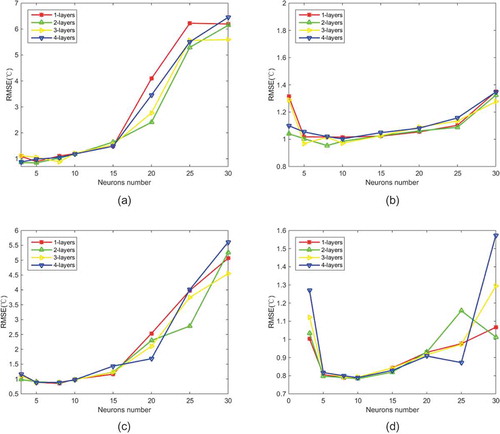
Figure 6. Predictive effect of the model on electrical conductivity at different depths: (a) station #1, (b) station #3, (c) station #5 and (d) station #7.

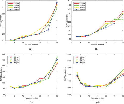
By analysing the data changes through Figs. 5 and 6, it is found that the prediction accuracy indication (RMSE) first increases and then decreases as the number of hidden layer neurons increases. This indicates that the model has been over-fitted with the increase of the number of neurons in the hidden layer and more neurons in the hidden layer are not as good as possible. Furthermore, the results show that a 2- or 3-layer model achieved good results in water temperature and electrical conductivity data fitting.

3.5 Comparison of different model prediction results

In order to verify the effectiveness of the improved model in predicting the water quality of virtual sites, three shallow neural network models, BPNN, ELM and WELM, and two deep ELM models, ELM-DAE and ELM-CDAE, were run with the parameters in each model as described in the last section. Under the same conditions, the prediction results are shown in Figs. 7 and 8.

Figure 7. Prediction of water temperature for four virtual monitoring stations by different models: (a) station #1, (b) station #3, (c) station #5 and (d) station #7.

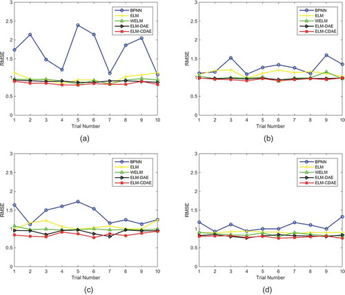
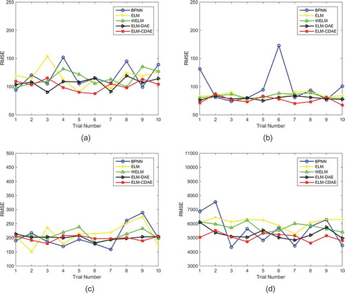
Figure 8. Predictions of electrical conductivity for four virtual monitoring stations by different models: (a) station #1, (b) station #3, (c) station #5 and (d) station #7.

By analysing Figs. 7 and 8, the following observations are made:

1. The RMSE of the water temperature predicted by the ELM-based models is smaller than that predicted by the BPNN model. The stability of ELM-based models is also better than that of the BPNN model. This means that the ELM-based model is more suitable for water temperature prediction than the BPNN model, especially for Station #1. In addition, deeper models perform better than shallow ELM models, such as ELM and WELM, because the deep ELM models can extract richer information from water quality data in shallow networks, especially for Station #5.

2. As can be seen from Fig. 8(a,b), the RMSE of the ELM-based model is mostly lower than that of the BPNN model in the 10 trials at stations #1 and #3. It is clear that the ELM-based models are more suitable for forecasting electrical conductivity at stations #1 and #3 than the BPNN models. From the prediction results of stations #5 and #7, it is seen that the prediction results of the BPNN model are better than those of the traditional shallow ELM model, but the difference between the results of the BPNN model and the deep ELM model is not particularly large. However, a defect that the BPNN model has is poor stability and it is difficult to converge, which was exposed in the 10 repeated trials. For example, the RMSE of the Experiment 6 for Station #3 is much larger than that of the other experiments, which means that the BPNN falls into local optimum too early. Besides, experiments 8 and 9 for Station #5 and the experiments 1 and 2 for Station #7 also show this flaw in the BPNN.

Furthermore, the average of the 10 experimental results indicated by the performance metrics and as well as the classical OK method are tested in this paper. The experimental results are shown in Tables 3 and 4, from which the following useful observations can be made:

Table 3. Prediction results of different models for water temperature at different stations.

Station		BPNN	ELM	WELM	ELM-DAE	ELM-CDAE	OK
#1	RMSE (°C)	1.7189	0.9773	0.9185	0.8983	0.8405	2.798
	MAE (°C)	1.0583	0.7194	0.6758	0.6637	0.6411	2.063
	MAPE	0.0451	0.0295	0.0266	0.0234	0.0213	0.0663
	R	0.9082	0.9763	0.9735	0.9791	0.9815	0.8753
#3	RMSE (°C)	1.2791	1.1179	1.0003	0.9729	0.9541	2.413
	MAE (°C)	0.8258	0.7763	0.7538	0.7331	0.7024	1.5731
	MAPE	0.0337	0.0321	0.0307	0.0314	0.0301	0.0787
	R	0.9543	0.9657	0.9713	0.9727	0.9718	0.9041
#5	RMSE (°C)	1.3894	1.0785	0.9948	0.9255	0.8514	2.7359
	MAE (°C)	0.9997	0.8549	0.8217	0.7758	0.7543	1.7247
	MAPE	0.0399	0.0337	0.0313	0.0301	0.0285	0.0613
	R	0.9366	0.9599	0.9667	0.9673	0.9681	0.8816
#7	RMSE (°C)	1.0788	0.911	0.855	0.8177	0.7908	1.8168
	MAE (°C)	0.8186	0.6504	0.6403	0.6107	0.6083	1.3510
	MAPE	0.0330	0.0262	0.0218	0.0204	0.0181	0.0687
	R	0.9710	0.9797	0.9783	0.9831	0.9854	0.9237

Table 4. Prediction results of different models for electrical conductivity at different stations.

Station		BPNN	ELM	WELM	ELM-DAE	ELM-CDAE	OK
#1	RMSE (μmho/cm)	118.135	117.224	114.847	106.724	104.525	143.156
	MAE (μmho/cm)	89.7867	84.9835	80.1753	80.2135	78.1056	93.5135
	MAPE	0.1493	0.1424	0.1352	0.1208	0.1187	0.1978
	R	0.3539	0.3555	0.3617	0.3728	0.3912	0.3357
#3	RMSE (μmho/cm)	98.6134	83.9665	83.3498	79.4622	76.1201	113.576
	MAE (μmho/cm)	65.5835	58.0681	57.8143	55.1486	54.0759	71.3698
	MAPE	0.1099	0.0968	0.0912	0.0854	0.0813	0.3113
	R	0.4062	0.4317	0.4389	0.4573	0.4644	0.3684
#5	RMSE (μmho/cm)	204.368	211.980	208.867	200.499	198.221	213.524
	MAE (μmho/cm)	162.476	161.596	158.478	153.547	151.354	160.516
	MAPE	0.1639	0.1670	0.1631	0.1518	0.1501	0.1733
	R	0.6142	0.6706	0.6973	0.7054	0.7113	0.6541
#7	RMSE(μmho/cm)	5590.92	6105.26	5784.17	5290.65	5060.73	5718.15
	MAE(μmho/cm)	3717.49	4507.06	4153.74	3687.15	3493.24	3947.56
	MAPE	3.0142	0.6635	0.6139	0.5896	0.4984	0.8638
	R	0.6428	0.7104	0.7253	0.7205	0.7319	0.5182

1. For water temperature forecasting results, the R values predicted by the neural network models are all more than 0.9 (Table 3), which means that the change in the prediction results in the virtual monitoring sites is consistent with that of the observed values. Besides, the results of the task for conductivity at stations #5 and #7 also show good performance. These experiments may give us a useful suggestion that some monitoring parameters of virtual monitoring sites can be stopped in the future, because the actual values of these parameters can be obtained by using the predicted results of relevant sites. However, the interpolation result for conductivity at statopms #1 and #2 shows that the R values are small, only about 0.4, which indicates that the prediction result is not ideal and monitoring of conductivity at these sites may no longer be optimized.

2. It is worth noting the prediction results of stations #5 and #7. For Station #5, the average of the results of 10 experimental trials show that the performance of the BPNN is better than that of the shallow ELM models, but inferior to that of the deep ELM models. Besides, the MAPE of the results at Station #7 is much more than 1, which indicates that there is a great gap between the prediction results of the BPNN and the observation values, even more than that of the OK method. Therefore, it is not recommended to use the BPNN to predict the conductivity at Station #7.

3. Compared with classical spatial interpolation algorithms such as the OK method, artificial neural networks such as the BPNN and ELM-based models are better when interpolating the water temperature at virtual sites. When predicting the actual value of electrical conductivity, the ANNs are also better than the OK method in most cases, except at Station #7. In addition, as indicated by the four performance indicators, the improved model proposed in this paper has higher prediction accuracy than the other models for its higher feature extraction ability.

4 Conclusion

A new deep ELM model for obtaining water quality data of an optimized monitoring network at a virtual monitoring station is presented. The model was divided into two parts: the first part was formed by stacking ELM-CDAE, which enables the whole model to extract more robust features from water quality data between different monitoring sites. In order to enhance the generalization capability of the model for virtual water quality prediction, the second part was realized by WELM, which uses the ratio of the current quarter sample size to the total sample size as the weight of the current sample. Finally, monthly water temperature and conductivity data from eight monitoring stations near Zengwen River in Taiwan collected from 22 January 2002 to 5 December 2017 were used to verify the effectiveness and the parameters in the model were selected by the cross-validation method. The water temperature forecasting results show that ANN models are better than the OK method, and the proposed method is superior to the other ELM-based models. For the prediction of conductivity at different virtual sites, the three shallow ANN models (BPNN, ELM, WELM) provided the most suitable sites. Besides, the OK method also showed better accuracy than the BPNN for the prediction task of Station #7, but it was worse than the ELM-based models. For the two water quality datasets, the deep ELM model performed well and the modified model was better, providing a good method to obtain water quality data of a virtual site for an optimized monitoring network.

In the future work, the influence of historical data length of each reference station will be discussed and then the water quality at a virtual monitoring station may be predicted.

Disclosure statement

No potential conflict of interest was reported by the authors.

Additional information

Funding

This study is supported by International Science and Technology Cooperation Program of Zhejiang Province for Joint Research in High-tech Industry [No. 2016C54007], National Key R&D Program of China [No. 2016YFC0201400], Leading Talents of Science and Technology Innovation in Zhejiang Provincial Ten Thousands Plan [No. 2019R52040], Provincial Key R&D Program of Zhejiang Province [No. 2017C03019] and National Natural Science Foundation of China and Zhejiang Joint Fund for Integrating of Informatization and Industrialization [No. U1509217].

Notes

¹ https://wq.epa.gov.tw/Code/Report/DownloadLis-t.aspx.

References

- Antanasijević, D., et al., 2017. A novel SON2-based similarity index and its application for the rationalization of river water quality monitoring network. River Research & Applications, 34 (1), 144–152. doi:10.1002/rra.3231
- Chapman, D.V., et al., 2016. Developments in water quality monitoring and management in large river catchments using the Danube River as an example. Environmental Science & Policy, 64 (5), 141–154. doi:10.1016/j.envsci.2016.06.015
- Chunping, O., et al., 2012. Coupling geostatistical approaches with PCA and fuzzy optimal model (FOM) for the integrated assessment of sampling locations of water quality monitoring networks (WQMNs). Journal of Environmental Monitoring Jem, 14 (12), 3118–3128. doi:10.1039/c2em30372h
- Deng, W.Y., et al., 2010. Research on extreme learning of neural networks. Chinese Journal of Computers, 33 (2), 279–287. doi:10.3724/SP.J.1016.2010.00279
- Do, H.T., et al., 2012. Design of sampling locations for mountainous river monitoring. Environmental Modelling & Software, 27 (2), 62–70. doi:10.1016/j.envsoft.2011.09.007
- Earle, R. and Blacklocke, S., 2008. Master plan for water framework directive activities in Ireland leading to River basin management plans. Desalination, 226 (1), 134–142. doi:10.1016/j.desal.2007.02.103
- Guigues, N., Desenfant, M., and Hance, E., 2013. Combining multivariate statistics and analysis of variance to redesign a water quality monitoring network. Environ Sci Process Impacts, 15 (9), 1692–1705. doi:10.1039/c3em00168g
- Huang, G.B., et al., 2012. Extreme learning machine for regression and multiclass classification. IEEE Trans Syst Man Cybern B Cybern, 42 (2), 513–529. doi:10.1109/TSMCB.2011.2168604
- Huang, G.B., Zhu, Q.Y., and Siew, C.K., 2006. Extreme learning machine: theory and applications. Neurocomputing, 70 (1), 489–501. doi:10.1016/j.neucom.2005.12.126
- Jia, X. and Du, H., 2016. Contractive ML-ELM for invariance robust feature extraction. In: Proceedings of ELM-2015 Volume 2. Cham: Springer, 203–208.
- Jiang, Y., et al., 2013. Analysis of spatial distribution of goundwater quality in Huaihe river basin. In: 2013 21st International Conference on Geoinformatics. Kaifeng, China: IEEE, 1–7.
- Juan, P.R., 2003. Neural networks for spatial interpolation of meteorological data. In: 3rd Conference on Artificial Intelligence Applications to the Environmental Science. Boulder, Colorado: American Meteorological Society, 60–68.
- Karamouz, M., et al., 2009a. Design of River water quality monitoring networks: a case study. Environmental Modeling & Assessment, 14 (6), 705–714. doi:10.1007/s10666-008-9172-4
- Karamouz, M., et al., 2009b. Design of on-line river water quality monitoring systems using the entropy theory: a case study. Environmental Monitoring & Assessment, 155 (1–4), 63–81. doi:10.1007/s10661-008-0418-z
- Kasun, K.L.C., et al., 2013. Representational learning with ELMs for big data. IEEE Intelligent Systems, 28 (6), 31–42.
- Khashei-Siuki, A. and Sarbazi, M., 2015. Evaluation of ANFIS, ANN, and geostatistical models to spatial distribution of groundwater quality (case study: Mashhad plain in Iran). Arabian Journal of Geosciences, 2 (8), 903–912. doi:10.1007/s12517-013-1179-8
- Kovács, J., et al., 2014. Classification into homogeneous groups using combined cluster and discriminant analysis. Environmental Modelling & Software, 57 (5), 52–59. doi:10.1016/j.envsoft.2014.01.010
- Laaha, G., Skøien, J.O., and Blöschl, G., 2012a. Comparing geostatistical models for river networks. Geostatistics Oslo 2012, ( Springer Netherlands), 45 (2), 543–553.
- Laaha, G., et al., 2013. Spatial prediction of stream temperatures using top-kriging with an external drift. Environmental Modeling & Assessment, 18 (6), 671–683. doi:10.1007/s10666-013-9373-3
- Laaha, G., Skøien, O.J., and Blöschl, G., 2012b. Spatial prediction on river networks: comparison of top‐kriging with regional regression. Hydrological Processes, 28 (2), 315–324. doi:10.1002/hyp.9578
- Lee, C., et al., 2014. Efficient method for optimal placing of water quality monitoring stations for an ungauged basin. Journal of Environmental Management, 132 (1), 24–31. doi:10.1016/j.jenvman.2013.10.012
- Li, B., McClendon, R.W., and Hoogenboom, G., 2004. Spatial interpolation of weather variables for single locations using artificial neural networks. Transactions of the ASAE, 47 (2), 629–637. doi:10.13031/2013.16026
- Li, J., et al., 2013. Use of genetic-algorithm-optimized back propagation neural network and ordinary kriging for predicting the spatial distribution of groundwater quality parameter. International Conference on Graphic and Image Processing, 8768 (5), 87684V.
- Liu, Y., Feng, X., and Zhou, Z., 2015. Multimodal video classification with stacked contractive autoencoders. Signal Processing, 120 (4), 761–766. doi:10.1016/j.sigpro.2015.01.001
- Mavukkandy, M.O., Karmakar, S., and Harikumar, P.S., 2014. Assessment and rationalization of water quality monitoring network: a multivariate statistical approach to the Kabbini River (India). Environmental Science & Pollution Research, 21 (17), 10045–10066. doi:10.1007/s11356-014-3000-y
- Maymandi, N., Kerachian, R., and Nikoo, M.R., 2018. Optimal spatio-temporal design of water quality monitoring networks for reservoirs: application of the concept of value of information. Journal of Hydrology, 558 (10), 328–340. doi:10.1016/j.jhydrol.2018.01.011
- Mehrjardi, R.T., Jahromi, M.Z., and Heidari, A., 2008. Spatial distribution of groundwater quality with geostatistics (Case study: yazd-Ardakan plain). World Applied Sciences Journal, 4 (1), 455–462.
- Mitrović, T., et al., 2019. Virtual water quality monitoring at inactive monitoring sites using Monte Carlo optimized artificial neural networks: a case study of Danube River (Serbia). Science of the Total Environment, 654 (8), 1000–1009. doi:10.1016/j.scitotenv.2018.11.189
- Philippopoulos, K. and Deligiorgi, D., 2012. Application of artificial neural networks for the spatial estimation of wind speed in a coastal region with complex topography. Renewable Energy, 38 (1), 75–82. doi:10.1016/j.renene.2011.07.007
- Prandtl, L., 1925. Z. angew. Math. Mech, 55 (5), 136–139.
- Reyjol, Y., et al., 2014. Assessing the ecological status in the context of the European water framework directive: where do we go now? Science of the Total Environment, 497 (1), 332–344. doi:10.1016/j.scitotenv.2014.07.119
- Rifai, S., et al., 2011. Contractive auto-encoders: explicit invariance during feature extraction. In: Proceedings of the 28th International Conference on International Conference on Machine Learning. Bellevue, Washington, USA: International Machine Learning Society, 833–840.
- Rizo-Decelis, L.D., Pardo-Igúzquiza, E., and Andreo, B., 2017. Spatial prediction of water quality variables along a main river channel, in presence of pollution hotspots. Science of the Total Environment, 55 (4), 276–290. doi:10.1016/j.scitotenv.2017.06.145
- Sabzipour, B., Asghari, O., and Sarang, A., 2017. Evaluation and optimal redesigning of river water-quality monitoring networks (RWQMN) using geostatistics approach (case study: Karun, Iran). Sustainable Water Resources Management, 45 (2), 1–17.
- Shahabi, M., et al., 2016. Spatial modeling of soil salinity using multiple linear regression, ordinary kriging and artificial neural network methods. Archives of Agronomy & Soil Science, 63 (2), 151–160. doi:10.1080/03650340.2016.1193162
- Sotiropoulos, D.G., Kostopoulos, A.E., and Grapsa, T.N., 2002. A spectral version of Perry’s conjugate gradient method for neural network training. Proceedings of 4th GRACM Congress on Computational Mechanics, 1 (5), 291–298.
- Tanos, P., et al., 2015. Optimization of the monitoring network on the River Tisza (Central Europe, Hungary) using combined cluster and discriminant analysis, taking seasonality into account. Environmental Monitoring and Assessment, 187 (9), 575. doi:10.1007/s10661-015-4777-y
- Villas-Boas, M.D., Olivera, F., and Azevedo, J.P.S.D., 2017. Assessment of the water quality monitoring network of the Piabanha River experimental watersheds in Rio de Janeiro, Brazil, using autoassociative neural networks. Environmental Monitoring & Assessment, 189 (9), 439. doi:10.1007/s10661-017-6134-9
- Vincent, P., et al., 2010. Stacked denoising autoencoders: learning useful representations in a deep network with a local denoising criterion. Journal of Machine Learning Research, 11 (12), 3371–3408.
- Wang, H., et al., 2015. Optimal Design of River Monitoring Network in Taizihe River by Matter Element Analysis. Plos One, 10 (5), 1455–1465.
- Wang, Y.B., et al., 2014. Spatial pattern assessment of river water quality: implications of reducing the number of monitoring stations and chemical parameters. Environmental Monitoring & Assessment, 186 (3), 1781–1792. doi:10.1007/s10661-013-3492-9
- Yang, X. and Jin, W., 2010. GIS-based spatial regression and prediction of water quality in river networks: A case study in Iowa. Journal of Environmental Management, 91 (10), 1943–1951. doi:10.1016/j.jenvman.2010.04.011
- Yingchun, F., et al., 2013. GIS and ANN-based spatial prediction of DOC in river networks: a case: study in Dongjiang, Southern China. Environmental Earth Sciences, 68 (5), 1495–1505. doi:10.1007/s12665-012-2177-y
- Zhang, N., Ding, S., and Shi, Z., 2016. Denoising Laplacian multi-layer extreme learning machine. Neurocomputing, 171 (3), 1066–1074. doi:10.1016/j.neucom.2015.07.058
- Zong, W., Huang, G., and Chen, Y., 2013. Weighted extreme learning machine for imbalance learning. Neurocomputing, 101 (2), 229–242. doi:10.1016/j.neucom.2012.08.010