Joint frequency analysis and uncertainty estimation of coupled rainfall–runoff series relying on historical and simulated data

ABSTRACT

Joint frequency analysis and quantile estimation of extreme rainfall and runoff (ERR) are crucial for hydrological engineering designs. The joint quantile estimation of the historical ERR events is subject to uncertainty due to the errors that exist with flow height measurements. This study is motivated by the interest in introducing the advantages of using Hydrologic Simulation Program-Fortran (HSPF) simulations to reduce the uncertainties of the joint ERR quantile estimations in Taleghan watershed. Bivariate ERR quantile estimation was first applied on P_AMS-Q_SIM pairs and the results were compared against the historical rainfall–runoff data (P_AMS-Q_obs). Student’s t and Frank copulas with respectively Gaussian-P3 and Gaussian-LN3 marginal distributions well suited to fit the P_AMS-Q_obs and P_AMS-Q_SIM pairs. Results revealed that confidence regions (CRs) around the p levels become wider for P_AMS-Q_obs compared to P_AMS-Q_SIM, indicating the lower sampling uncertainties of HSPF simulations compared to the historical observations for bivariate ERR frequency analysis.

KEYWORDS:

• extreme rainfall–runoff
• HSPF model
• copula
• bivariate frequency analysis
• uncertainty analysis

Editor A. Fiori Associate editor K. Kochanek

1 Introduction

Joint frequency analysis of extreme rainfall and runoff (ERR) events provides valuable information for design, maintenance and risk analysis of hydraulic structures (Zhang and Singh 2012). The joint probability and conditional return periods (RT) of the ERR variables are also important for the deployment of water harvesting systems. The joint quantile estimation of the ERR has been one of the main difficulties faced by the hydrologists because of the different stochastic nature of the rainfall and runoff process. To alleviate this issue, copulas (Sklar 1959) have been suggested to derive the joint probability distribution of the historical ERR data independently from their marginal distributions (Vandenberghe et al. 2010, Fu and Butler 2014). Copula functions provide efficient algorithms for construction of the joint probability distribution of several variables with different marginal distributions (Favre et al. 2004).

Copulas have been widely applied for bivariate frequency analysis of either extreme rainfall (Joo et al. 2012, Jun et al. 2017, Jhong and Tung 2018, Liu et al. 2018a) or runoff attributes (Xu et al. 2017, Liu et al. 2018b, Tosunoglu and Singh 2018). However, the joint frequency analysis of the coupled extreme rainfall–runoff (ERR) is rarely investigated in the literature. Zhang and Singh (2012) applied copulas for joint ERR quantile estimation based on the historical ERR pairs at near Riesel and Cuyahoga rivers in Texas. They showed that Placket copula is the most appropriate copula for modelling the rainfall–runoff data.

The joint frequency analysis of historical ERR data is subject to the input data uncertainty. Montanari (2010) indicated that sampling uncertainty is one of the major source of uncertainties in hydrological frequency analyses. Dung et al. (2015) investigated bivariate flood peak-volume frequency analysis in Mekong Delta in Cambodian and Vietnamese and indicated that sampling uncertainty is the major source of uncertainty in flood frequency analysis while model selection and parameter estimation methods are of only minor importance. For ERR frequency analysis there is a need to the long-time continuous rainfall and streamflow data. Although the rainfall data are readily available, there are difficulties in measuring runoff especially during the flooding events. In some cases, the floods are impossible to be measured leading to the time-lapses in the streamflow time series. They may also be measured incorrectly, resulting in outliers in the original data sets. There is still another source of uncertainties in streamflow data measurements. The streamflow data are indirect measurements of the flow heights which are transformed to the corresponding discharge through the rating curves (Saghafian et al. 2014). This may result in uncertainty which arose due to the peak flows extrapolation from the rating curves (Domeneghetti et al. 2012). This study contributed to fill an important gap in bivariate ERR frequency analysis through investigating the possibility of replacing the historical observations with hydrologic model simulations for ERR frequency analysis in poorly gauged watersheds.

To investigate this hypothesis, uncertainty of the bivariate frequency analysis of the ERR events relying on historical observations and hydrologic model simulations was assessed. Hydrological Simulation Program-Fortran (HSPF) model (Bicknell et al. 1997) is considered in this study as it is among the few models with the capability of accurately reproducing the hydrologic and hydraulic storm events (Donigian et al. 1995). The HSPF model uses numerous parameters that can be adjusted to achieve an accurate representation of the watershed (Fonseca et al. 2014). There have been successful applications of the HSPF model for different watersheds in all over the world (Johnson et al. 2003, Albek et al. 2004, Borah and Bera 2004, Singh et al. 2005, Xie and Lian 2013, Lampert and Wu 2015, Seong et al. 2015). In the present study, the advantages of using the HSPF model simulations instead of historical observations are investigated for bivariate ERR frequency analysis. For this purpose, we attempted to explore how the uncertainty of the ERR quantiles changes by replacing the historical observations with HSPF simulations.

For accounting, the uncertainties of the historical and simulated ERR quantiles a non-parametric resampling algorithm based on the bootstrap method is considered in this study. Bootstrap method is a type of resampling algorithm that relies on the random sampling with replacement of the original data (Hesterberg et al. 2005). The main advantages of the bootstrap method over the other resampling approaches are its high accuracy (DiCiccio and Efron 1996) and simplicity (García-Soidán et al. 2014) which provides straightforward way to derive estimates of the standard errors and confidence intervals for parameters of the distribution (Chen et al. 2016, Zhang et al. 2018). Zhang et al. (2018) indicated that the bootstrap method is useful when the assumption of the normal distribution is not ascertained for marginal variables, such as for ERR series in this study. Thus, the bootstrap algorithm is used for uncertainty estimation of the ERR quantiles in this study. The use of bootstrap method for univariate quantile estimations is not difficult as there are many applications of that for univariate hydrological data analyses in the literature (for, e.g. Lall and Sharma 1996, Vogel and Shallcross 1996, Fortin et al. 1997, Mirzaei et al. 2013, 2014, 2015, Huang et al. 2016, Jaramillo et al. 2018, Zhang et al. 2018, Ng et al. 2019). In this study, we adopted the bootstrap algorithm in a bivariate context using the Acceptance-Rejection algorithm to explore the uncertainties of the joint ERR quantiles. For this purpose, we investigated uncertainties of the multivariate models with two parameter copulas that have not yet been investigated earlier. The main objectives of this study are (i) to explore the most appropriate copulas to fit the historical and simulated ERR time series, (ii) to compare the joint quantiles of the historical and simulated ERR data and (iii) to identify the uncertainties of the ERR quantiles using the non-parametric bootstrap method.

2 Description of the study case

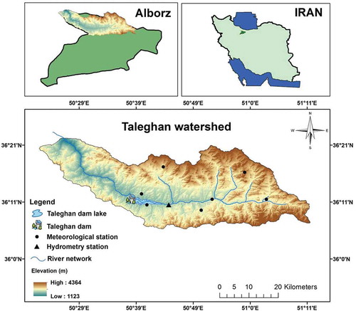
The case study is Taleghan watershed which is located 100 km far from the capital. The watershed with a drainage area of 800 km² and an average altitude of 2753 m is located between 50°20′E–51°10′E and 36°5′N–36°23′N (Fig. 1). The climate of the watershed is Mediterranean, with an average temperature of 4.48°C and a mean annual rainfall of 701 mm (Dodangeh et al. 2017). The Taleghan Dam was built on the Taleghan River and created a lake with an area of 12 km² and a total volume of 420 × 10⁶ m³ downstream of Galinak village. This dam is located 135 km northwest of Tehran and supplies 150 × 10⁶ m³ of drinking water of Tehran and Alborz provinces. The reservoir is also the main source of water supply for agricultural activities in the Qazvin Plain (Dodangeh et al. 2019).

Figure 1. Location of the study area.

Flooding is a predominant phenomenon in this area causing much damage annually. For example, the last flooding event in April 2019 caused a loss of US$1,200,000 through damage to roads, livestock, gardens, and farms. The rainfall–runoff relationship is highly non-linear in this region due to the variability of the moisture in the watershed. Depending on the humidity conditions of the watershed, low amounts of precipitation accompanied by massive floods and vice versa. Thus, univariate frequency analysis of either the extreme rainfall or runoff is not sufficient for optimal utilization of the water resources. Therefore, the joint frequency analysis and quantile estimation of the ERR series are considered in this study by applying copulas. Bivariate quantile estimation uncertainties are also compared between the historical floods and HSPF simulations.

3 Methodology

3.1 HSPF model

3.1.1 HSPF model description

The HSPF model (Bicknell et al. 1997) is one of the semi-distributed hydrology simulation models developed for continuous simulation of watershed’s quantitative and qualitative hydrological process. The HSPF model is an integrated version of three elementary models namely the Agricultural Runoff Management Model (ARM) of the US Environmental Protection Agency (EPA), the EPA Nonpoint Source Runoff Model (NPS) and the Hydrologic Simulation Program (Dodangeh et al. 2017).

Hydrological simulation in this model is handled by three application modules: PERLAND, IMPLAND and RCHRES. The process of water movement, infiltration, interception and evapotranspiration on pervious surfaces is embedded in the PERLAND module. This module also simulates the snow accumulation and melting process. The IMPLAND module has the same functionality as the PERLAND but for impervious surfaces, such as built-up surfaces where the infiltration rate is insignificant. The runoff generated on pervious and impervious surfaces is routed by the RCHRES module (Donigian et al. 1995).

3.1.2 Data preparation and assimilation

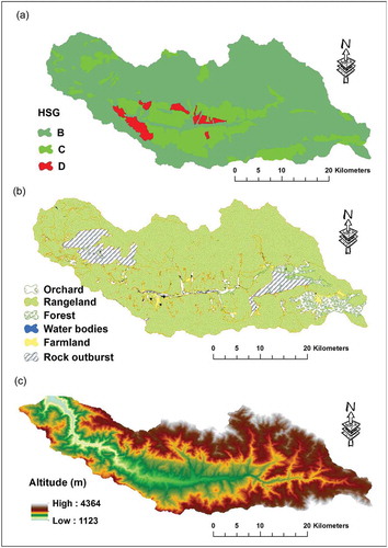
A GIS database including the hydrologic soil groups (HSG), land-use map and digital elevation model (DEM) (Fig. 2) with 30 m × 30 m resolution were prepared in .shp format in the BASINs4.1 interface. A land use/land cover map was obtained from the Landsat 7 satellite imagery with 30 m × 30 m resolution. A DEM was also downloaded from the US Geological Survey (earthexplorer.usgs.gov). The daily rainfall and temperature data of seven meteorological and synoptic stations (Fig. 1) were acquired for the period 1979–2012. The daily scale streamflow data of Galinak station (#17-035) was also obtained for the same period. The available meteorological and discharge data were imported into a watershed data management (WDM) file to provide the input time series required by the WinHSPF program. All of the spatial and input time series were stored in a user control input (.uci) file and then transferred to the WinHSPF interface to perform the model calibration. The WinHSPF component, distributed with BASINS4.1 (Bicknell et al. 1996), was used for calibration of the model. The HSPF model calibrated and validated against the daily streamflow data of Galinak station for the period 1995–2005. After the calibration, the model is used for daily river flow simulation in a 33-year period (1979–2012).

Figure 2. Spatial data used for HSPF model calibration: (a) hydrologic soil groups (HSG), (b) land-use map and (c) digital elevation model (DEM).

3.1.3 Model performance evaluation

For assessment of the degree-of-fit of the HSPF model, various performance evaluation measures are considered. There is a wide range of performance evaluation measures used for hydrological modelling evaluation. For performance evaluation of the HSPF model, the most commonly used evaluation measures including root-mean-square error (E_RMS), Nash-Sutcliffe efficiency (E) (Nash and Sutcliffe 1970), coefficient of determination (R²) (Wright 1921) and percent bias (P_BIAS) which have been verified as the most informative measures (Krause et al. 2005) are used in this study:

(1) $R^2=1-\frac{\sum _{\mathrm{i}=1}^n{\left(Q_{\mathrm{o}\mathrm{b}\mathrm{s}}-Q_{\mathrm{S}\mathrm{I}\mathrm{M}}\right)}^2}{\sum _{\mathrm{i}=1}^n{(Q_{\mathrm{o}\mathrm{b}\mathrm{s}}-{\bar{Q}}_{\mathrm{o}\mathrm{b}\mathrm{s}})}^2}$(1)

(2) $E=1-\left[\frac{1/n\sum _{\mathrm{i}=1}^n{(Q_{\mathrm{o}\mathrm{b}\mathrm{s}}-Q_{\mathrm{S}\mathrm{I}\mathrm{M}})}^2}{1/n\sum _{\mathrm{i}=1}^n{(Q_{\mathrm{o}\mathrm{b}\mathrm{s}}-{\bar{Q}}_{\mathrm{o}\mathrm{b}\mathrm{s}})}^2}\right]$(2)

(3) $E_{\mathrm{R}\mathrm{M}\mathrm{S}}=\sqrt{\sum _{\mathrm{i}=1}^n\frac{{(Q_{\mathrm{o}\mathrm{b}\mathrm{s}}-Q_{\mathrm{S}\mathrm{I}\mathrm{M}})}^2}{n}}$(3)

(4) $P_{\mathrm{B}\mathrm{I}\mathrm{A}\mathrm{S}}=100\times \left[\frac{{\sum }^{(}{Q}_{\mathrm{S}\mathrm{I}\mathrm{M}}-Q_{\mathrm{o}\mathrm{b}\mathrm{s}})}{{\sum }^{Q_{\mathrm{o}\mathrm{b}\mathrm{s}}}}\right]$(4)

where Q_SIM is daily simulated flow, Q_obs is daily observed flow, ${\bar{Q}}_{\mathrm{o}\mathrm{b}\mathrm{s}}$ is the average observed flow of the simulation period and n is the number of days. Values of R² and E close to 1 and of E_RMS and P_BIAS close to 0 imply a perfect fit of the model (Yan et al. 2014).

3.2 Copula-based bivariate statistical models

Copula theory was introduced by Sklar (1959) to model the stochastic nature of the multi-dimensional process by derivation of multivariate distribution functions from the univariate marginal distributions. For the bivariate cases, such as in this study, the joint cumulative distribution function (JCDF) F_X,Y (x,y) of the random variables X and Y are estimated using the copula function as follows:

(5) $F_{X,Y}(x,y)=C(F_X(x),F_Y(y))$(5)

where C explains the copula function and F_X(x) and F_Y(y) are the marginal cumulative density functions (cdfs) of the random variable X and Y, estimated using the univariate probability distributions. The parameterization of the marginal distributions is conducted independently and the copula parameter is estimated based on the tail dependence of the marginal variables. Equation (50) can be rewritten in the form:

(6) $F_{X,Y}(x,y,\theta )=C(F_X(x,{\theta }_x),F_Y(y,{\theta }_y),{\theta }_c)$(6)

where θ_x and θ_y represent the parameters of the univariate marginal distributions, θ is the parameter of bivariate model and θ_c is the copula parameter (Dung et al. 2015).

Various copula functions have been introduced to use in the literature (Joe 1997, Nelsen 2006, Sungur and Nelson 2006). In this study Archimedean copulas, Student’s t and Plackett copulas are considered to model the joint stochastic nature of the ERR process. The non-parametric Kendall’s tau estimation method can be used for simple parameter copula families (Zhang and Singh 2006, Mirakbari et al. 2010, Janga Reddy and Ganguli 2012). However, for two-parameter copula families, such as Student’s t copula, the maximum likelihood estimation method is more appropriate (Joe 1997) and hence is used in this study. For identifying the most appropriate copula which best-fits the ERR time series, the Akaike information criterion (AIC) and the Cramer-von Mises test are employed.

3.3 Bivariate quantile uncertainty estimation

Stochastic modelling of either univariate or multivariate frequency analysis of hydrological variables comes with uncertainties. Sampling uncertainty (SU) is among the major sources of the uncertainties that influence the frequency analysis of the stochastic variables. The bootstrap algorithm (Efron 1979) with owing the advantages of simplicity and high accuracy (Zhang et al. 2018) has emerged to be used for uncertainty analysis of the random variables. The bootstrap algorithm is referred to the tests or metrics that rely on random sampling with replacement of the original data (Zhang et al. 2018). There are many applications of this algorithm in the literature for univariate hydrological data analyses (for, e.g. Lall and Sharma 1996, Vogel and Shallcross 1996, Jaramillo et al. 2018). Uncertainty analysis of univariate quantile estimations is not difficult task as it can be easily quantified by following a simple process of data resampling approach (Chowdhury and Stedinger 2007).

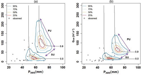
Unlike the univariate quantile estimation, there are more difficulties with bivariate quantile estimation uncertainty, especially for two-parameter copulas as discussed in this study. Bivariate quantile estimations suffer from the uncertainties which arise not only due to the parameter estimation of the marginal distributions but also due to the estimation of the dependence structure between the marginal variables. There is still additional uncertainty for bivariate quantile estimation which results from the design event selection on the p-level curves. There are indefinite combinations of variables x and y (ERR variables) on a given p-level curve which have the same probability of occurrence. These combinations have different implications for engineering applications (Salvadori and Michele 2011).

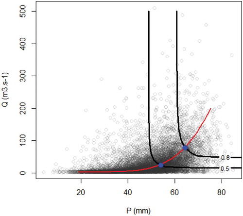
As illustrated in Fig. 3, there are indefinite pairs of ERR events (P-Q pairs) on the quantile curves with the same hazard level (p = 0.5 and 0.8) and different likelihoods. This means that, although all of the ERR pairs on a given p-level curve mathematically share the same probability of occurrence, they do not physically have the same likelihood. For example, both of the 80–30 and 50–500 P-Q pairs on the p = 0.5 curve have mathematically the same probabilities of occurrence (p = 0.5) however the likelihood of them is different in the real world. Likewise, the probability of occurrence of both of the 80–50 and 60–500 pairs is p = 0.8 but they have different likelihoods. The point with the highest density on the p-level curves is the event with the highest likelihood and is considered as a design event in hydrologic engineering applications. For estimation of this point, a line that best fits the dependence between the x and y variables is plotted. The intersection of this line with the p-level curve identifies the design event. The more accurate estimation of this point along the p-level curves results in the reduced uncertainties of the bivariate quantiles estimation. Design event estimation is one of the major sources of uncertainties in bivariate quantile estimations, which is not the case in univariate frequency analysis.

3.3.1 Acceptance-rejection sampling (ARS) algorithm

The univariate frequency analysis is not subjected to such uncertainties because of one-one mapping association between the quantiles and their associated probabilities. The acceptance-rejection sampling (ARS) algorithm (Casella et al. 2008, Martino and Míguez 2010) is employed to estimate the bivariate design event on the p-level curves. Figure 3 demonstrates the design event estimation on the 0.5 and 0.8 probability levels (the blue points) corresponding to F_XY using the ARS algorithm:

Figure 3. Design events estimation on quantile curves of p = 0.5 and p = 0.8.

1. Sample B realizations, u_j (j = 1, …, B) from a uniform distribution in the range [p,1].

2. Calculate the corresponding value v_j such that (u_j,v_j) ϵ $L_p^F$

3. Approximate auxiliary realization ξ_j from a uniform distribution in the range [0,1].

4. Estimate the density of the copula (u_j,v_j) for the B simulated pairs.

5. Reject the simulated pairs if $\frac{c\left(u_j,v_j\right)}{\mathrm{m}\mathrm{a}{\mathrm{x}}_j\left\{c\left(u_j,v_j\right)\right\}}<{\xi }_j$

6. For estimation of a design event along the p-level curve corresponding to F_XY, the u_j value is sampled from a uniform distribution in [0,p] (Serinaldi 2013).

3.3.2 Bootstrap method with ARS algorithm

To estimate the CRs around the p-level curves using the bootstrap method with the ARS algorithm for sampling from the p-level curves, the following steps are followed:

1. Set the number of bootstrap samples to a sufficiently large number N_b (N_b = 500).

2. Generate N_b bootstrap samples by sampling with replacement from the observed x-y pairs. The size of all N_b bootstrap samples should be identical to the size of the original sample of observed x-y pairs.

3. Fit N_b separate copulas to the generated N_b bootstrap samples.

4. Generate a random integer number in the range [1, N_b], and select the corresponding copula from the fitted copulas.

5. Simulate a point along the p-level curve (at a specific p-level, for instance, p = 0.95) of the copula selected in Step 4. Such a point is also referred to as the p th quantile. Points along a p -level curve are simulated using an acceptance-rejection algorithm.

6. Repeat steps 4 and 5 N_s = 50 000 times.

7. Identify the confidence ranges around the p-level curves using the N_s points.

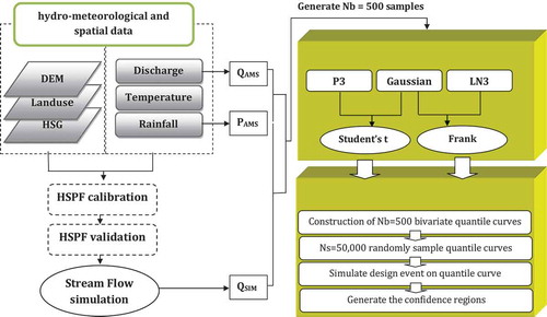
In order to investigate the hypothesis of the research concerning the uncertainty reduction of the hydrological frequency analysis using the hydrologic model simulation instead of historical data, Taleghan Watershed is selected. The HSPF model calibrated and validated against the daily streamflows of the watershed during the period 1995–2005. The calibrated model was then applied for long time river flow simulations for the period 1979–2012. Annual maximum series of precipitation (P_AMS) with their corresponding observed runoff (Q_obs) and HSPF model simulations (Q_SIM) are used to construct the bivariate statistical models using copula functions. The joint frequency analysis and quantile estimation of the P_AMS-Q_obs and P_AMS-Q_SIM pairs are conducted using the best-fit copulas. The bootstrap method was applied for uncertainty analysis of the quantile estimations of the P_AMS-Q_obs and P_AMS-Q_SIM to test the hypothesis of the research. The flowchart of the proposed methodology for joint frequency analysis and uncertainty assessment of the historical and simulated ERR is presented in Fig. 4.

Figure 4. Flowchart of the study.

4 Results and discussion

4.1 HSPF model application

The HSPF model calibrated against the daily streamflow data of the Galinak station for a 5-year period (1995–2000). Parameters of the model calibrated based on the advises of the HSPExp expert system (Lumb et al. 1994) and guidelines of BASINs technical Note 6 (BASINS 2012). The HSPF model incorporates a wide range of parameters for the representation of the physical process of the watersheds (Fonseca et al. 2014). Table 1 outlines some key parameters and their calibrated values of the HSPF model. The result of the model calibration against the observed daily streamflow of the Galinak station is illustrated in Fig. 5. As can be seen from Fig. 5, the simulated daily runoff during the winter season (January–March) is over estimated. The peak flows on the other hand are underestimated in spring rainy season (April–June). In the Taleghan Watershed, much of the spring peak flows in river are attributed to the snowmelt runoff. The mountainous regions in highlands of the watershed act as a water saving system, storing snowpack in the cold season (January–March) and releasing the water into the river when the snowpack begins to melt. The effect of the snowmelt on flooding may be even accelerated by the excessive rainfall on melting snow during the spring. The large peaks in Fig. 5 are mainly the result of snow melt, underestimated by the HSPF model. The model assumed that the rainfall immediately transformed to runoff in cold season. This leads to the over estimation of the streamflow in January–March, as shown in Fig. 5.

Figure 5. HSPF calibration before adjusting the KMELT parameter.

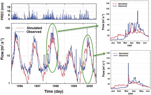
Table 1. The main parameters of the HSPF model calibrated for streamflow simulation. in: inch.

			Possible values
Parameter	Definition	Unit	Min	Max	Calibrated range
INFILT	Index to infiltration capacity	in/h	0.001	0.5	0.4
AGWRC	Base groundwater recession	none	0.85	0.999	0.971–0.996
LZSN	Lower zone nominal soil moisture storage	in	2	15	5–5.5
UZSN	Upper zone nominal soil moisture storage	in	0.05	2	1.12–2
DEEPFR	Fraction of groundwater inflow to deep recharge	none	0	0.5	0–0.01
INTFW	Interflow inflow parameter	none	1	10	1
IRC	Interflow recession parameter	none	0.3	0.85	0.3
BASETP	Fraction of remaining ET from baseflow	none	0	0.2	0–0.02
LZETP	Lower zone ET parameter	none	0.1	0.9	0.1–0.4
AGWETP	Fraction of remaining Et from active ground water	none	0	0.2	0.1
KMELT	Degree-day factor	in/d	0.14	0.2	0.14–0.2

Moreover, the peak streamflow in the late spring (April–June) is underestimated because the snowmelt runoff is overlooked. The KMELT key parameter is considered to simulate the snow accumulation and melting process to improve the winter and spring streamflow simulations. Figure 6(a) illustrates the daily streamflow simulation after KMELT parameter calibration. As shown in Fig. 6(a), the KMELT parameter calibration resulted in a better simulation of the daily streamflow in cold season and peak streamflow in spring. Fonseca et al. (2014) gained acceptable results in daily streamflow simulation of Lis river basin in Portugal without KMELT parameter calibration. Amirhossien et al. (2015) also reported a successful application of the HSPF model without the KMELT snow melting parameter in Balkhlichai basin in northern Iran. The Lis and Balkhlichai river basins are coastal basins with hydro-climate characteristics different from the Taleghan Watershed. The results of the model validation (2000–2005) against the observed daily streamflow of Galinak station are displayed in Fig. 6(b). As shown in Fig. 6(b), there is a close agreement between the model simulations and observed daily streamflow during the calibration and validation periods. The results of the performance evaluation of the model based on the subjective criteria are also outlined in Table 2. The statistical measures of Table 2 confirms a high degree of correlation (R² > 0.7) between the observed and simulated runoff during the calibration and validation periods. The E_RMS values are <10 m³ s⁻¹ for all of the daily, monthly and annual streamflow simulations. The P_BIAS values were in the range 1.8–15.96 and E exceeded 0.7 suggesting that the model attained acceptable results in predicting the runoff. The Nash-Sutcliffe efficiency (E) and R² values exhibit a high degree of sensitivity on peak flows as they are squared deviations of the predicted values from the observations (Krause et al. 2005). The results presented in Table 2 indicate that the model performance is similar for both calibration and validation phases implying that the calibrated parameters in Table 1 demonstrate a good representation of the Taleghan Watershed. Therefore, the calibrated model is used to simulate the long-term daily streamflow of the watershed for the period 1979–2012. The values of Q_SIM corresponding to the P_AMS were extracted from the daily streamflow predictions to construct the bivariate statistical models using copulas.

Figure 6. (a) calibration (1995–2000) and (b) validation (2000–2005) of the HSPF model after adjusting the KMELT parameter.

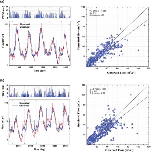
Table 2. HSPF model evaluation using the commonly used performance evaluation criteria.

	R^2	PBIAS (%)	ERMS (m^3 s^−1)	E
Calibration (1995–2000)
Daily	0.83	1.8	5.62	0.83
Monthly	0.87	5.99	4.62	0.86
Annual	0.84	1.8	1.77	0.83
Validation (2000–2005)
Daily	0.79	5.85	6.7	0.78
Monthly	0.86	9.49	5.2	0.85
Annual	0.91	5.84	2.9	0.81
Simulation (1979–2012)
Daily	0.71	15.3	8.3	0.66
Monthly	0.82	15.96	6.1	0.78
Annual	0.74	15.27	9.8	0.70

4.2 Joint modelling of ERR using copulas

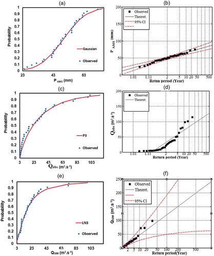
For construction of the joint probabilistic model of the ERR, extreme rainfall (P_AMS) and corresponding historical and simulated runoff (Q_obs, Q_SIM) were separately fitted by various univariate probability distributions. The maximum likelihood estimation method is used to estimate the fitted probability distributions and then the best-fit distributions were identified based on the least AIC values. Table 3 shows that the Gaussian, P3, and LN3 are the most appropriate distributions to fit P_AMS, Q_obs and Q_SIM. Wang (2007) also emphasized on the efficiency of the P3 and LN3 as the most appropriate univariate distributions to fit peak streamflow in Des Moines River basin tributaries. There are also successful applications of these probability distributions for flood frequency analysis in Saf (2009) and Sarhadi et al. (2012). The best-fit models were used to estimate the cumulative density functions (cdf) of the P_AMS, Q_obs and Q_SIM.

Table 3. Goodness-of-fit criteria for various univariate marginal distributions fitted to the selected data time series. AIC: Akaike Information Criterion; KS: Kolmogorov-Smirnov.

		KS
Data	Distribution family and estimated parameters	Statistic	p value	AIC
PAMS	Gaussian (γ = 0.88, μ = 49.56, σ = 12.32)	0.09	0.9	262
Qobs	P3 (α = 0.59, β = 41.9, γ = 3.48)	0.11	0.15	293
QSIM	LN3 (γ = 0.03, μ = 2.69, σ = 0.9)	0.08	0.95	269

Figure 7 illustrates the cdfs and quantiles estimation plots of the P_AMS, Q_obs and Q_SIM time series. As illustrated in Fig. 7, the observed data fitted well by the selected probability distributions. The Q_obs and Q_SIM have the return periods of less than 50 years; however, for the same quantile values, the return periods of the Q_SIM are slightly larger than those of the Q_obs indicating that frequency analysis of peak flows based on the HSPF simulations yields the lower risk comparing to the historical observations.

Figure 7. Fitting univariate probability distributions to P_AMS, Q_obs and Q_SIM: (a), (c) and (e) cdf plots; and (b), (d) and (f) probability plots.

In order to construct the bivariate statistical models, the theoretical cdfs of the P_AMS-Q_obs and P_AMS-Q_SIM pairs were fitted by various copulas with different tail dependence characteristics. Table 4 outlines the used copulas with associated parameter values and the degree-of-fit test measures. The Cramer-von Mises test results indicate that all of the bivariate models are acceptable at the 5% significance level. However, according to the AIC values, Student’s t (AIC = ‒8.71) and Frank (AIC = ‒4.87) copulas outperformed other candidate copulas to fit, respectively, P_AMS-Q_obs and P_AMS-Q_SIM pairs. Lourme and Maurer (2017) also indicated the high capability of Student’s t copula for capturing the phenomenon of dependant extreme values. This copula gives asymptotic dependence in the tail even for negative or zero correlations. The Frank copula has the capability of capturing both negative and positive correlations in ERR dependence. Zhang and Singh (2012) also affirmed the good performance of the Frank copula to fit annual maximum rainfall and corresponding runoff of the Riesel River watershed.

Table 4. Summary of copula goodness-of-fit test results for the Cramer-von Mises criterion (Sn), and associated p values calculated from a parametric bootstrap test (10,000 bootstrap samples). The best-fit copulas are indicated in bold.

Data	Copula family	Sn	p-value	Estimated parameter	AIC
PAMS-Qobs	Student’s t	0.04	0.84	0.46 1.72	–8.71
	Clayton	0.05	0.84	0.88	–8.35
	Plackett	0.04	0.86	4.14	–8.37
	Gumbel	0.05	0.84	1.44	–5.21
	Frank	0.04	0.85	2.96	–7.50
	Gaussian	0.05	0.84	0.46	–5.80
PAMS-QSIM	Student’s t	0.16	0.12	0.33 30	–3.67
	Clayton	0.04	0.15	0.66	–4.08
	Plackett	0.03	0.36	3.42	–4.60
	Gumbel	0.06	0.11	1.16	–1.65
	Frank	0.03	0.27	2.55	–4.87
	Gaussian	0.04	0.08	0.39	–3.76

The best-fit copulas were used to construct the bivariate t-Gaussian-P3 and Frank-Gaussian-LN3 models for ERR frequency analysis, as discussed in the following.

4.3 ERR frequency analysis

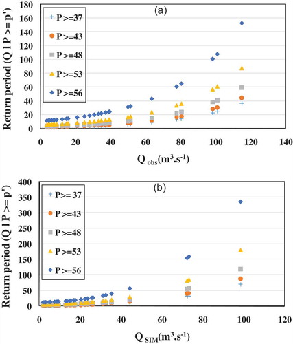
The bivariate statistical models, t-Gaussian-P3 and Frank-Gaussian-LN3 were used for ERR frequency analysis and quantile estimation of the historical and simulated data. The joint CDFs of the historical and simulated ERR pairs were estimated using the constructed models. Figure 8 shows the bivariate quantile curves of the P_AMS-Q_obs and P_AMS-Q_SIM for various probability levels and return periods. As the figure shows, most of the historical P_AMS-Q_obs events have return periods less than 50 years. However, the return periods of the P_AMS-Q_SIM events exceed 200 years. Figure 9 illustrates the conditional return periods of Q_obs and Q_SIM for different levels of P_AMS. For the same P_AMS, Q_SIM exhibits longer return periods compared to Q_obs. For example, for P ≥ 56 mm, the return period of Q_SIM ≈ 100 m³ s⁻¹ is 350 years, which is longer than that for Q_obs (=100 years). This indicates a lower risk of ERR occurrence when using hydrological modelling simulations instead of historical observations.

Figure 8. Joint probability and return periods (RT) of P_AMS-Q_obs and P_AMS-Q_SIM: (a) and (c) joint probability plots; and (b) and (d): RT plots.

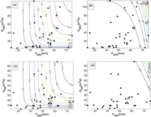
Figure 9. Conditional RT of (a) Q_obs given P_AMS, (b) Q_SIM given P_AMS.

4.4 Uncertainty analysis

Uncertainty evaluation of the ERR quantiles is also carried out using the nonparametric bootstrap method. Figure 10 shows the bivariate quantiles of P_AMS-Q_SIM and associated uncertainties for p levels of 0.5, 0.8, 0.9, 0.95, 0.98 and 0.99. The black dots in Fig. 10 are the N_s = 50 000 ERR quantiles calculated through the bootstrap algorithm. The 25–95% confidence regions (CRs) display uncertainties of the P_AMS-Q_SIM quantile estimations. The parallel extent of the CRs along the p-level curves explains the uncertainties that resulted from the model selection and their associated parameter estimations (PU). Besides, the extent of the CRs along the 45° line demonstrates the sampling uncertainty (SU). Figure 11 shows the bivariate quantile estimation uncertainties of the P_AMS-Q_obs pairs. Comparing Figs. 10 and 11, it is revealed that PU is similar for various p-level curves of the Frank copula; however, it is getting smaller when moving from low to higher hazard levels for the Student’s t copula. This is due to the fact that there are substantial differences between the tail dependence structure of the Frank and Student’s t copulas. Student’s t copula has positive tail dependency both in the lower and upper tails (tau_LU = 0.42) which narrowed the distribution of P_AMS-Q_obs coincidence along the higher hazard levels (PU) while for Frank copula with no tail dependency the PU is similar for all of the p-level curves. The decrease in PU with increasing the hazard levels in Student’s t copula implies the good efficiency of this copula to describe the dependence structure of the investigated data.

Figure 10. Uncertainty estimation of bivariate quantiles of P_AMS-Q_SIM at different probability levels of p = 0.5–0.99.

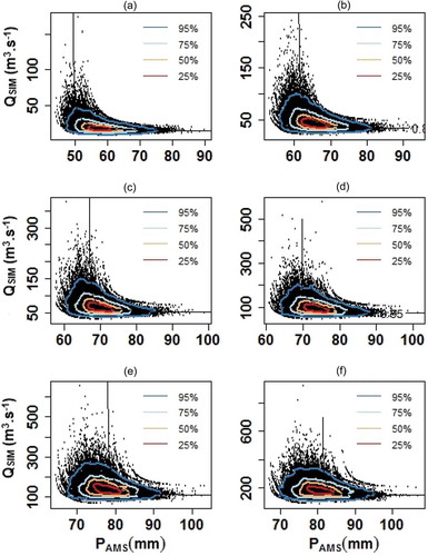
Figure 11. Uncertainty estimation of bivariate quantiles of P_AMS-Q_obs at different probability levels of p = 0.5–0.99.

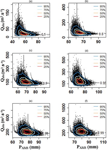
Both Figs. 10 and 11 show that the sampling uncertainty along the 45° line is increased for larger p levels; however, increasing SU with increasing p levels in the Frank copula is not as sensible as in the Student’s t copula. This is because of the different dependence structure of P_AMS-Q_obs and P_AMS-Q_SIM at the upper tail. As illustrated in Fig. 12, the increasing dispersion of P_AMS-Q_obs occurs more strongly compared to the P_AMS-Q_SIM when moving from low to higher p levels. This is reasonable because the dependence of P_AMS-Q_SIM is less disturbed by the environmental noise in comparison to the P_AMS-Q_obs which resulted in lower data density and then greater uncertainty of the P_AMS-Q_obs quantiles in the upper tail. There is still another major uncertainty source in the frequency analysis of the historical data concerning the peak flows measurements. This uncertainty is due to the errors occurred either during the measuring peak flow heights or extrapolating the peak flow discharges from the flow heights on the rating curves (Domeneghetti et al. 2012). In this study, we solved this type of uncertainty by applying a conceptual hydrologic model for reproducing the peak flow discharges from the extreme rainfall values. Since the rainfall measurement is easy and less error prone than the flow measurements, reproducing the peak flow discharges from the rainfall measurements noticeably reduced the uncertainty of the ERR frequency analysis (Fig. 12). Although the hydrological model calibration may be influenced by the historical flood measurements, calibrating the model against the measured low to medium discharges will prevent the carrying over the uncertainties into the calibration phase. The results of this study demonstrate that the joint frequency analysis of the ERR quantiles based on the HSPF model simulations resulted in less uncertainties of the design event estimations. The use of hydrological model simulations for the purposes of hydrological frequency analysis is more cost-effective compared to the direct frequency analysis of the historical streamflow. This study may encourage practitioners to accommodate their calculations based on the hydrological model simulations to reduce the uncertainties and economic costs of the water resources management projects.

Figure 12. Comparison of uncertainties between (a) historical data and (b) HSPF simulation.

5 Summary and conclusions

This study investigated the risk assessment and uncertainty analysis of the ERR quantiles based on historical data and HSPF model simulations. The long-term daily streamflow simulation of the Taleghan Watershed (1979–2012) was conducted using the HSPF model. The annual maximum series of precipitation (P_AMS) and corresponding historical (Q_obs) and simulated runoff (Q_SIM) were fitted by various univariate and copula functions. The following observations were made:

1. The bivariate t-Gaussian-P3 model is identified as the best model to fit the P_AMS-Q_obs pairs, while the Frank-Gaussian-LN3 model better fitted the P_AMS-Q_SIM pairs. The tail dependency in P_AMS-Q_SIM is less influenced by the environmental noises so it was better fitted by the Frank copula with a uniform tail dependence structure.

2. Unlike the univariate frequency analysis of extreme rainfall and runoff, the results of the joint ERR frequency analysis showed that for the same hazard values, the bivariate quantiles of the P_AMS-Q_obs are higher than the simulated pairs indicating on the lower risk estimation when using HSPF model simulations instead of the direct frequency analysis of historical data.

3. The results indicate that sampling uncertainties are noticeably reduced for HSPF model simulations comparing to the frequency analysis of historical data. The HSPF model preserved the dependence structure between the ERR variables while reducing the sampling uncertainties through eliminating the errors associated with flow height measurements and peak flow discharge extrapolation on the rating curves. As the risk overestimation leads to the waste of investment, the HSPF model would be affordable for uncertainty reduction of the hydrological frequency analysis of ERR events.

4. Although the sampling uncertainty of joint quantile estimations is reduced for HSPF model simulations compared to the historical data; however, quantitative values of different uncertainty source are not provided in this study. The future works are encouraged to provide quantitative values for various uncertainty sources to explore how much uncertainties can be reduced by using the hydrological modelling simulations instead of the direct frequency analysis of historical data.

Acknowledgements

The authors would like to thank Iran Meteorological Organization (IRIMO) and Iran Water Resources Management Company (IWRMC) for providing the basic hydro-climatic data. We also thank two anonymous reviewers and the associate editor for their comments.

Disclosure statement

No potential conflict of interest was reported by the authors.

References

- Albek, M., Öǧütveren, Ü.B., and Albek, E., 2004. Hydrological modeling of Seydi Suyu watershed (Turkey) with HSPF. Journal of Hydrology, 285, 260–271. doi:10.1016/j.jhydrol.2003.09.002
- Amirhossien, F., et al., 2015. A comparison of ANN and HSPF models for runoff simulation in Balkhichai River watershed, Iran. American Journal of Climate Change, 4, 203–216. doi:10.4236/ajcc.2015.43016
- BASINS, 2012. Basins technical note 6: Estimating hydrology and hydraulic parameters for HSPF. Bibliogov. USA, BASINS.
- Bicknell, B.R., et al., 1997. Hydrological Simulation Program–Fortran, user’s manual for version 11. US Environmental Protection Agency, Technical Report EPA/600/R-97/080. CA, USA, University of the Pacific.
- Bicknell, B.R., et al., 1996. Hydrological Simulation Program - Fortran user’s manual for release 11. US Environmental Protecion Agency.
- Borah, D.K. and Bera, M., 2004. Watershed-scale hydrologic and nonpoint-source pollution models: review of applicantions. Transactions of the ASAE., 47(3), 789–803.
- Casella, G., Robert, C.P., and Wells, M.T., 2008. Generalized accept-reject sampling schemes. doi:10.1214/lnms/1196285403
- Chen, S., et al., 2016. Constructing confidence intervals of extreme rainfall quantiles using Bayesian, bootstrap, and profile likelihood approaches. Science China Technological Sciences. doi:10.1007/s11431-015-5951-8
- Chowdhury, J.U. and Stedinger, J.R., 2007. Confidence interval for design floods with estimated skew coefficient. Journal of Hydraulic Engineering. doi:10.1061/(asce)0733-9429(1991)117:7(811)
- DiCiccio, T.J. and Efron, B., 1996. Bootstrap confidence intervals. Statistical Science. doi:10.1214/ss/1032280214
- Dodangeh, E., et al., 2017. Usability of the BLRP model for hydrological applications in arid and semi-arid regions with limited precipitation data. Modeling Earth Systems and Environment, 3 (2), 539–555. Springer Nature. doi:10.1007/s40808-017-0312-1
- Dodangeh, E., et al., 2019. Data-based bivariate uncertainty assessment of extreme rainfall–runoff using copulas: comparison between annual maximum series (AMS) and peaks over threshold (POT). Environmental Monitoring and Assessment, 191 (2). Springer Nature. doi:10.1007/s10661-019-7202-0
- Domeneghetti, A., Castellarin, A., and Brath, A., 2012. Assessing rating-curve uncertainty and its effects on hydraulic model calibration. Hydrology and Earth System Sciences, 16, 1191–1202. doi:10.5194/hess-16-1191-2012
- Donigian, A.S.Jr., et al., 1995. Chapter 12: Hydrological Simulation Program – FORTRAN. In V.P. Singh (Ed.) Computer Models of Watershed Hydrology. Highland Ranch, CO, Water Resources Publications, pp. 395–442.
- Dung, N.V., et al., 2015. Handling uncertainty in bivariate quantile estimation - an application to flood hazard analysis in the Mekong Delta. Journal of Hydrology, 527, 704–717. doi:10.1016/j.jhydrol.2015.05.033
- Efron, B., 1979. Bootstrap methods: another look at the jackknife. The Annals of Statistics, 7, 1–26. doi:10.1214/aos/1176344552
- Favre, A.C., et al., 2004. Multivariate hydrological frequency analysis using copulas. Water Resources Research. 40. doi:10.1029/2003WR002456
- Fonseca, A., et al., 2014. Watershed model parameter estimation and uncertainty in data-limited environments. Environmental Modelling & Software, 51, 84–93. doi:10.1016/j.envsoft.2013.09.023
- Fortin, V., Bernier, J., and Bobée, B., 1997. Simulation, Bayes, and bootstrap in statistical hydrology. Water Resources Research, 33, 439–448. doi:10.1029/96WR03355
- Fu, G. and Butler, D., 2014. Copula-based frequency analysis of overflow and flooding in urban drainage systems. Journal of Hydrology, 510, 49–58. Elsevier B.V. doi:10.1016/j.jhydrol.2013.12.006
- García-Soidán, P., Menezes, R., and Rubiños, Ó., 2014. Bootstrap approaches for spatial data. Stochastic Environmental Research and Risk Assessment, 28, 1207–1219. doi:10.1007/s00477-013-0808-9
- Hesterberg, T., et al., 2005. Bootstrap methods and permutation tests. In: Introduction to the practice of statistics. doi:10.1002/wics.182
- Huang, Y.F., Mirzaei, M., and Amin, M.Z.M., 2016. Uncertainty quantification in rainfall intensity duration frequency curves based on historical extreme precipitation quantiles. Procedia Engineering, 154, 426–432. doi:10.1016/j.proeng.2016.07.425
- Janga Reddy, M. and Ganguli, P., 2012. Application of copulas for derivation of drought severity-duration-frequency curves. Hydrological Processes, 26, 1672–1685. doi:10.1002/hyp.8287
- Jaramillo, F., et al., 2018. Dominant effect of increasing forest biomass on evapotranspiration: interpretations of movement in Budyko space. Hydrology and Earth System Sciences, 22, 567–580. doi:10.5194/hess-22-567-2018
- Jhong, B.C. and Tung, C.P., 2018. Evaluating future joint probability of precipitation extremes with a copula-based assessing approach in climate change. Water Resources Management, 32, 4253–4274. doi:10.1007/s11269-018-2045-y
- Joe, H., 1997. Multivariate models and dependence concepts. Monographs on Statistics and Applied Probability, New York, Chapman and Hall.
- Johnson, M.S., et al., 2003. Application of two hydrologic models with different runoff mechanisms to a hillslope dominated watershed in the northeastern US: A comparison of HSPF and SMR. Journal of Hydrology, 284, 57–76. doi:10.1016/j.jhydrol.2003.07.005
- Joo, K., Shin, J., and Heo, J.-H., 2012. Bivariate frequency analysis of rainfall using copula model. Journal of Korea Water Resources Association, 45 (8), 827–837. doi:10.3741/JKWRA.2012.45.8.827
- Jun, C., et al., 2017. Bivariate frequency analysis of rainfall intensity and duration for urban stormwater infrastructure design. Journal of Hydrology, 553, 374–383. doi:10.1016/j.jhydrol.2017.08.004
- Krause, P., Boyle, D.P., and Bäse, F., 2005. Comparison of different efficiency criteria for hydrological model assessment. Advanced Geosciences, 5, 89–97. doi:10.5194/adgeo-5-89-2005
- Lall, U. and Sharma, A., 1996. A nearest neighbor bootstrap for resampling hydrologic time series. Water Resources Research, 32, 679–693. doi:10.1029/95WR02966
- Lampert, D.J. and Wu, M., 2015. Development of an open-source software package for watershed modeling with the Hydrological Simulation Program in Fortran. Environmental Modelling & Software, 68, 166–174. doi:10.1016/j.envsoft.2015.02.018
- Liu, C., et al., 2018a. Multivariate frequency analysis of urban rainfall characteristics using three-dimensional copulas. Water Science and Technology. doi:10.2166/wst.2018.103
- Liu, Z., et al., 2018b. Hydrological risk analysis of dam overtopping using bivariate statistical approach: a case study from Geheyan Reservoir, China. Stochastic Environmental Research and Risk Assessment, 32, 2515–2525. doi:10.1007/s00477-018-1550-0
- Lourme, A. and Maurer, F., 2017. Testing the Gaussian and Student’s t copulas in a risk management framework. Economic Modelling, 67, 203–214. doi:10.1016/j.econmod.2016.12.014
- Lumb, A.M., McCammon, R.B., and Kittle, J.L., Jr., 1994. Users manual for an expert system (HSPEXP) for calibration of the Hydrological Simulation Program-Fortran. USGS Water-Resources Investigations Report, 94, 4168. doi:10.1111/j.1600-065X.2011.01092.x
- Martino, L. and Míguez, J., 2010. Generalized rejection sampling schemes and applications in signal processing. Signal Processing, 90, 2981–2995. doi:10.1016/j.sigpro.2010.04.025
- Mirakbari, M., Ganji, A., and Fallah, S.R., 2010. Regional bivariate frequency analysis of meteorological droughts. Journal of Hydrologic Engineering, 15, 985–1000. doi:10.1061/(asce)he.1943-5584.0000271
- Mirzaei, M., et al., 2013. Model calibration and uncertainty analysis of runoff in the Zayanderood River basin using Generalized Likelihood Uncertainty Estimation (GLUE) method. Journal of Water Supply: Research and Technology-Aqua, 62, 309–320. doi:10.2166/aqua.2013.038
- Mirzaei, M., et al., 2015. Uncertainty analysis for extreme flood events in a semi-arid region. Natural Hazards, 78, 1947–1960. doi:10.1007/s11069-015-1812-9
- Mirzaei, M., et al., 2014. Quantifying uncertainties associated with depth duration frequency curves. Natural Hazards, 71, 1227–1239. doi:10.1007/s11069-013-0819-3
- Montanari, A., 2010. Uncertainty of hydrological predictions. In: Treatise on water science. doi:10.1016/B978-0-444-53199-5.00045-2
- Nash, J.E. and Sutcliffe, J.V., 1970. River flow forecasting through conceptual models part I — a discussion of principles. Journal of Hydrology, 10, 282–290. doi:10.1016/0022-1694(70)90255-6
- Nelsen, R.B., 2006. An introduction to copulas. New York, NY: Springer Science+Business Media, Inc. Available from: http://www.springerlink.com/content/q88865
- Ng, J.L., et al., 2019. Uncertainty analysis of rainfall depth duration frequency curves using the bootstrap resampling technique. Journal of Earth System Science. 128. doi:10.1007/s12040-019-1154-1
- Saf, B., 2009. Regional flood frequency analysis using L-moments for the West Mediterranean region of Turkey. Water Resources Management, 23, 531–551. doi:10.1007/s11269-008-9287-z
- Saghafian, B., Golian, S., and Ghasemi, A., 2014. Flood frequency analysis based on simulated peak discharges. Natural Hazards, 71, 403–417. doi:10.1007/s11069-013-0925-2
- Salvadori, G. and Michele, C.D., 2011. Estimating strategies for multiparameter multivariate extreme value copulas. Hydrology and Earth System Sciences, 15, 141–150. doi:10.5194/hess-15-141-2011
- Sarhadi, A., Soltani, S., and Modarres, R., 2012. Probabilistic flood inundation mapping of ungauged rivers: linking GIS techniques and frequency analysis. Journal of Hydrology, 458–459, 68–86. doi:10.1016/j.jhydrol.2012.06.039
- Seong, C., Herand, Y., and Benham, B.L., 2015. Automatic calibration tool for Hydrologic Simulation Program-FORTRAN using a shuffled complex evolution algorithm. Water. doi:10.3390/w7020503
- Serinaldi, F., 2013. An uncertain journey around the tails of multivariate hydrological distributions. Water Resources Research, 49, 6527–6547. doi:10.1002/wrcr.20531
- Singh, J., et al., 2005. Hydrological modeling of the Iroquois River watershed using HSPF and SWAT. Journal of the American Water Resources Association, 41, 343–360. doi:10.1111/j.1752-1688.2005.tb03740.x
- Sklar, A., 1959. Fonctions de répartition à n dimensions et leurs marges. Publications de l’Institut de Statistique de l’Université de Paris, 8, 229–231.
- Sungur, E.A. and Nelson, R.B., 2006. An introduction to copulas. Journal of the American Statistical Association. doi:10.2307/2669568
- Tosunoglu, F. and Singh, V.P., 2018. Multivariate modeling of annual instantaneous maximum flows using copulas. Journal of Hydrologic Engineering, 23, 04018003. doi:10.1061/(asce)he.1943-5584.0001644
- Vandenberghe, S., Verhoest, N.E.C., and Baets, B.D., 2010. Fitting bivariate copulas to the dependence structure between storm characteristics: a detailed analysis, based on 105 year 10 min rainfall. Water Resources Research. 46. doi:10.1029/2009WR007857
- Vogel, R.M. and Shallcross, A.L., 1996. The moving blocks bootstrap versus parametric time series models. Water Resources Research, 32, 1875–1882. doi:10.1029/96WR00928
- Wang, C., 2007. A joint probability approach for the confluence flood frequency analysis. Ames, IA: Iowa State University. Available from: http://gateway.proquest.com/openurl?url_ver=Z39.88-2004&rft_val_fmt=info:ofi/fmt:kev:mtx:dissertation&res_dat=xri:pqdiss&rft_dat=xri:pqdiss:1447555
- Wright, S., 1921. Correlation and causation.pdf. Journal of Agricultural Research. doi:10.2307/3966855
- Xie, H. and Lian, Y., 2013. Uncertainty-based evaluation and comparison of SWAT and HSPF applications to the Illinois River Basin. Journal of Hydrology, 481, 119–131. doi:10.1016/j.jhydrol.2012.12.027
- Xu, Y., Huang, G., and Fan, Y., 2017. Multivariate flood risk analysis for Wei River. Stochastic Environmental Research and Risk Assessment, 31, 225–242. doi:10.1007/s00477-015-1196-0
- Yan, C.A., Zhang, W., and Zhang, Z., 2014. Hydrological modeling of the Jiaoyi watershed (China) using HSPF model. The Scientific World Journal, 2014, 1–9. doi:10.1155/2014/672360
- Zhang, A., et al., 2018. Analysis of the influence of rainfall spatial uncertainty on hydrological simulations using the bootstrap method. Atmosphere, 9, 71. doi:10.3390/atmos9020071
- Zhang, L. and Singh, V.P., 2006. Bivariate flood frequency analysis using the copula method. Journal of Hydrologic Engineering, 11, 150–164. doi:10.1061/(asce)1084-0699(2006)11:2(150)
- Zhang, L. and Singh, V.P., 2012. Bivariate rainfall and runoff analysis using entropy and copula theories. Entropy, 14, 1784–1812. doi:10.3390/e14091784