Designing river water quality policy interventions with scarce data: the case of the Middle Tagus Basin, Spain

ABSTRACT

Anthropic pressures deteriorate river water quality, so authorities need to identify their causes and define corrective actions. Physically based water quality models are a useful tool for addressing physicochemical pollutants, but they must be calibrated with an amount of data that is often unavailable. In this study, we explore the characterization of a model to design corrective interventions in a context of sparse data. A calibration indicator that is both simple and flexible is proposed. This approach is applied to the Middle Tagus Basin in central Spain, where the physicochemical concentration of pollutants is above legal standards. We quantify the effects of the main existing pressures (discharge from wastewater treatment plants, agricultural diffuse pollution and a major inter-basin water transfer) on the receiving waters. In particular, the study finds that wastewater treatment plant effluent concentrations should be reduced to up to 0.65 mg/L of ammonium and 0.55 mg/L of phosphate to achieve the environmental goals. We propose and prioritize a set of policy actions that would contribute to the good status of surface water bodies in the region.

KEYWORDS:

• Water Framework Directive
• water quality
• Tagus Basin
• data scarcity
• modelling

Editor A. Castellarin Guest editor S. Uhlenbrook

1 Introduction

River banks have been a preferential area for human settlement since the early civilizations (Macklin and Lewin 2015). Suitable conditions such as water availability, land fertility due to nutrient-rich floods and ease of transport of goods (Vega et al. 1998, Di Baldassarre et al. 2013) have attracted high population densities in the vicinities of rivers. They have also entailed an increase in river pollution (Ward and Elliot 1995) and, as a result, continental water quality is worsening globally (Allaoui et al. 2015).

In places where deteriorating water quality threatens ecosystem sustainability, water authorities need to identify the causes and prescribe corrective actions. This is often defined through water quality models. There is a growing body of scholarly literature on the modelling of the ecological status of rivers and the effect of pressures caused by polluting agents (Thomann and Mueller 1987, Genkai-Kato and Carpenter 2005, Chapra 2008, Momblanch et al. 2015, Dodds and Smith 2016, Shrestha et al. 2016). Among other elements (biological and hydromorphological), physicochemical indicators are used to describe the concentrations of oxygen and nutrients that are compatible with the long-term sustainability of freshwater ecosystems. In the case of continental surface waters, the main pressures on water quality are present in the form of the urban wastewater, industrial pollution and nutrient-rich agricultural fertilizers. While point source pressures are easier to locate and quantify through direct measures at the discharge, diffuse pollution characterization poses complex challenges (Strömqvist et al. 2012, Epelde et al. 2015), leading to data demanding models, or qualitative output studies (Munafò et al. 2005, Zhang and Huang 2011).

Physically based models use water quality observations to understand the behaviour of river stretches (Fonseca et al. 2014, Keupers and Willems 2017, Hutchins and Bowes 2018). Typically, observations on a regular basis (daily, weekly) of flow and pollutant concentration for rivers and pollutant discharges have been used to characterize the model through performance indicators. For a given study area, these indicators compare river observations downstream with model output (simulated from river observations upstream and pollutant discharges along the study area). However, the available observations are often too sparse to allow such approach, and there is limited research investigating how to calibrate the models when data is not dense enough to correlate pressures and observations on similar dates. The first approach is to move away from physically based models and describe the process with empirically based regressions tailored for small sample sizes (Cohn et al. 1989). Due to the difficulty of interpreting the parameters in physically meaningful terms, other authors combine the two approaches and start from mechanistic models to which statistical methods are applied (Romanowicz et al. 2004, Wellen et al. 2014). Some scholars maintain the existing indicators, widening the data scale (monthly instead of daily) to adapt to the existing data (Tarawneh et al. 2016), while others combine this approach with annual mass balances (Zhao et al. 2010).

In this paper, we explore options to offer science-based support to water management decisions when the data observations are scarce. We propose a calibration technique that does not require a pair-wise comparison between pressures and receiving water status. This is achieved through the development of a goal function that exploits the statistical properties of the existing data.

The approach is applied to the Middle Tagus Basin, Spain, where surface waters fail to comply with the established quality standards. Adapting the methodology to the few observations available (four water quality observations per year), the study quantifies the effect of the existing pressures on river water quality. It also defines the infrastructure changes and the management decisions that are required to achieve or maintain the good status of the surface waters.

Understanding river water quality dynamics in this region is especially interesting for several reasons. Firstly, this area receives the wastewater of a highly populated urban region – the metropolitan region of Madrid – and the diffuse pollution from fertilized irrigated land, and has relatively low-flow rivers with limited capacity to dilute pollution. Wastewater treatment plants (WWTP) in the study area present a high efficiency in biological oxygen demand reduction but have an uneven record in nutrient reduction. The study thus explores the degree of additional nutrient reduction required to attain the environmental improvements. Secondly, a large interbasin water transfer (Tagus Segura Water Transfer) diverts a half of Tagus headstream waters to the Southeast of Spain. Currently, the quantity of water to be transferred is decided on a monthly basis, depending on the stored water volumes in the major reservoirs of the Tagus headwaters (MAPAMA 2014). The water transfer limits the capacity of Tagus River to dilute the pollution produced by the Madrid region. Previous studies have sought to understand the impact of the transfer (Morales Gil et al. 2005, San Martín 2011, Pellicer-Martínez and Martínez-Paz 2018) on water availability in the donor’s region but have not assessed its implications on water quality. A previous water quality study in the region of Madrid (Cubillo et al. 1992) has been outdated because of wastewater treatment infrastructure upgrades. It does not include the effect of the interbasin water transfer and does not issue policy recommendations on the required quality of WWTP effluents. A more recent study (Paredes et al. 2010) prescribes maximum pollutant concentration for the effluents but is restricted geographically to a subregion (the Manzanares River).

2 Materials

2.1 Study area

The study area includes several river stretches of the Middle Tagus Basin, including the lower course of the Jarama and Henares rivers, the Manzanares River from upstream the city of Madrid and the Tagus River from its confluence with the Jarama at Aranjuez (Fig. 1, T.0) to the city of Toledo (T.70).

Figure 1. Area of study. Arrow shows Tagus Segura water transfer. Positions (e.g. M.0) are labelled as “river code.kilometric distance from reference starting point”.

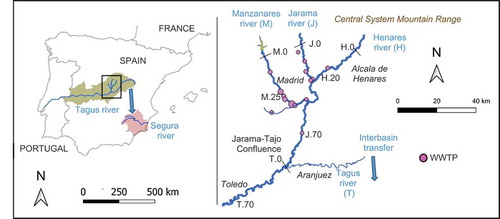
The study area has a Mediterranean climate with warm and dry summers, rated Csa in the Köppen-Geiger classification (Kottek et al. 2006). Average monthly temperatures range from 2.7 to 32.1ºC (AEMET 2018). Rainfall distribution is highly influenced by the presence of the Central System Mountain Range to the north of the study area (Durán Montejano 2016). The orographic effect implies that yearly precipitation varies from 1500 mm/year in the northern highlands, to below 400 mm/year in the midlands between Aranjuez and Toledo. Most water runoff is therefore generated in the headwaters. Precipitation shows also a strong seasonality, with wet winters (60 mm/month on average in the city of Madrid) and dry summers (10 mm/month). This seasonality has a major impact on the quantity and quality of circulating surface waters, and on agricultural irrigation practices.

Madrid urban area hosts more than 5.1 million people (INE 2018). Urban water demand amounts to 32 hm³/month (CHT 2015a) and is largely met by reservoirs in the Upper Jarama River (upstream of the area of study). Fifteen major WWTPs treat and discharge wastewater produced by domestic and industrial uses (Table 1). Total authorized discharge of WWTPs is 37 hm³/month, although normal operation flow is below this volume (CHT 2015b). Water withdrawal for irrigation amounts to 16 hm³/year (CHT 2015a). Groundwater and surface water bodies receive the surplus of nutrients of the fertilizers applied to 200,000 ha of agricultural land in the region (DGA 2017).

Table 1. Position (river code.distance from reference point) and average discharge of major WWTPs.

Position	WWTP	Discharging to	Average discharge (hm^3/month)
H.17	Alcala Este	Henares	0.3
H.21	Alcala Oeste		1.3
M.12	Viveros	Manzanares	1.7
M.24	China		2.6
M.27	Gavia		2.5
M.29	Butarque		3.2
M.34	Sur		7.3
M.37	A. Culebro		2.6
M.43	Suroeste		0.7
J.17	Valdebebas	Jarama upstream Henares confluence	0.7
J.24	Rejas		1.5
J.29	Torrejon		0.7
J.30	Casa Quemada		1.2
J.40	Velilla S. Antonio	Jarama downstream	0.2
J.68	Soto Gutierrez	Henares confluence	0.5
		Total	27.2

The average flow of Jarama River in its lower stretch ranges between 20 hm³/month in summer and 122 hm³/month in winter (MAPAMA 2018), and average flow in the Middle Tagus River ranges between 51 and 159 hm³/month.

Upstream of its confluence with the Jarama River, Tagus River is subject to a major interbasin water transfer that diverts an average of 30 hm³/month to the southeast of the Iberian Peninsula (Fig. 1).

2.2 Data collection

The data used in this study is collected from the following sources:

• River flow data from gauging stations (MAPAMA 2018): water flow data measured in 19 stations on a daily basis, available until 2015.

• Pollutant concentration from river water quality stations (CHT 2018): concentration of dissolved oxygen (DO), biological oxygen demand (BOD₅), ammonium (NH₄), nitrate (NO₃) and phosphate (PO₄) in the surface bodies of water, measured in 30 stations every 90 days, on average, from 2003 to 2017.

• WWTP effluent pollutant concentration from Tagus River Basin Authority: concentration of biological oxygen demand, ammonium, total nitrogen and total phosphorus from the WWTPs in the study area, measured every 60 days on average from 2009 to 2017.

• Digital elevation model DEM (IGN 2018) with a spatial resolution of 25 m.

• Rainfall (AEMET 2018). Daily precipitation for eight meteorological stations in the study area, series starting before year 2000.

• Nitrogen surplus: Nitrogen applied to the agricultural lands that is not taken by the crops. Yearly average from 2000 to 2013 per autonomous community (administrative region), reported by the authorities (DGA 2017), in accordance with the Directive 91/676/EEC.

In view of data availability, the 2009–2015 period is selected for being the most recent time span with a complete set of information for all the required variables.

The river flow data allows a description of the quantity of water in the system on a daily basis. The geographical distribution of the river quality stations is acceptable (with an average distance of 10 km between stations), but the number of observations per year does not allow a detailed characterization of the temporal distribution of the pollutant concentration. Only the annual average for agricultural pressures, six observations per year for WWTP effluents and four observations per year for river quality are available. This does not allow the definition of a continuous series of events where a particular observation of the concentration of pollutants in the river can be correlated to a particular observation of the pressures.

2.3 WWTP and diffuse pollution pressures

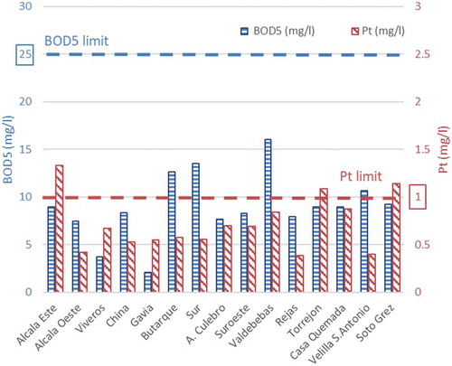
WWTP effluents are subject to Spanish regulations derived by the Urban Waste Water Treatment Directive (UWWTD) 91/271/EEC (Council of the European Communities 1991). In particular, effluent from WWTPs treating wastewater from over 100,000 equivalent inhabitants must have concentrations of total suspended solids (TSS) below 35 mg/L and a BOD₅ below 25 mg/L. Since the study area is declared as a catchment of an area sensitive to eutrophication by phosphorus, there is an additional limit of 1 mg/L for total phosphorus (Pt). By contrast, the area is not declared a catchment of an area sensitive to eutrophication by nitrogen, and there is no upper limit to nitrogenous compounds concentration by default. Figure 2 shows that virtually all WWTPs comply with these default limits (excess Pt is present in three smaller WWTPs, with a limited effect on receiving waters).

Figure 2. WWTP effluent concentrations (2009–2015 average). BOD5: biological oxygen demand, Pt: total phosphorus.

With respect to diffuse pollution coming from agricultural sources, only nitrogenous compounds are regulated. Unlike the UWWTD, Directive 91/676/CEE (concerning the protection of waters against pollution caused by nitrates from agricultural sources) does not impose upper limits to nitrate pollution. It only prescribes the monitoring of applied fertilizers, crop uptake, and nitrogen surplus. No specific calculation is required by the legislation to sort out which fraction of the nitrogen surplus is washed out in superficial runoff, and which fraction is leached to the aquifer. According to official reports (DGA 2017), total nitrogen surplus in the study area ranges between 8 and 28 kg/ha per year for the period 2009–2013. A fraction of this surplus will reach the surface waters through runoff. In the case of phosphorus, there is no equivalent to the agricultural nitrates directive to quantify the surplus generated by agriculture.

2.4 River water quality objectives and current situation

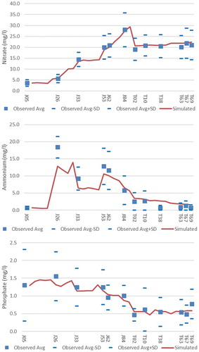
The Water Framework Directive (WFD) 2000/60/EC (European Parliament and Council 2000) describes the conditions to be fulfilled by surface water bodies to guarantee the sustainability of their ecosystems, i.e. to reach a good status. Figure 3 shows the observed (average +/− standard deviation) concentration of nutrients compared to the maximum limit established according to the WFD for Jarama River and Tagus River between Aranjuez and Toledo. Despite overall compliance of WWTP effluents to standard limits, there are pollutant concentrations in the receiving waters that are above the thresholds compatible with a good status. This points to the need for more stringent constraints on the polluting pressures.

Figure 3. Observed nutrient concentration and limits in legislation along the Jarama (J.05–J.84) and Tagus (T.00–T,70) rivers.

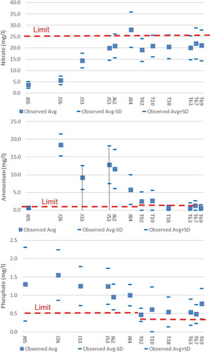
Nitrate concentration (Fig. 3) grows steadily along the Jarama River as it receives the WWTP effluents, diffuse pollution and the waters of the Henares and Manzanares rivers, then it decreases at the confluence with Tagus headwaters. The average concentration remains under the 25 mg/L limit for all the surface waters except for a minor noncompliance at the lower Jarama.

Ammonium concentration along the Jarama River is prone to substantial changes depending on the nature of the point loads. From a low concentration in the headwaters, effluents from non-nitrifying WWTPs in the upper middle Jarama force an upwards spike. Relatively low concentrations from Henares River contribute to water down these high values (at J.33 position, i.e. Jarama River, 33 km downstream of the reference point), but high ammonium loads from WWTPs in Manzanares River drive up the values at its confluence with the Jarama (J.53). Ammonium and phosphate concentrations remain above the limits for most of the river stretches in the study area.

3 Methodology

A water quality model is built to simulate the concentration of pollutants in the study area. Details are given in the Supplementary material. The model boundaries include the Jarama, Henares, Manzanares and Tagus river stretches that support the urban pressures. The upper border of the model is pushed upstream to a point where the rivers flow in near to pristine water quality conditions before major pressures are applied. The hydrological model takes account of average contributions from river headwaters measured in gauging stations at the upstream frontier, as well as local diversions, WWTP effluent discharges and contribution from soil runoff.

The water quality model is based on the RREA (Spanish acronym for “Rapid Response to the Ambient State”) model approach (Paredes-Arquiola 2018) for transport and fate of pollutants.

Point loads are introduced in the model at the authorized discharge locations of WWTPs. The concentration of pollutants in WWTP effluent is calculated from measurements at plant discharge.

For each river stretch, the corresponding sub-basin – or Exclusive Contribution Area (De Oliveira et al. 2016) – is calculated from the DEM using QGIS software (QGIS Development Team 2018). Since the diffuse load (nitrates and phosphates) for each sub-basin is unknown, the value introduced is calculated in the calibration stage correlating simulated and observed values. Only anionic nitrate mobility is modelled, since cationic ammonium is considered to be more electrically bonded to soil particles (García-Serrano et al. 2009). Since the total nitrogen surplus is known from European Union reports (DGA 2017), we will assume in our study that a particular fraction of this surplus reaches the surface water. In the case of phosphorus, we will assume that anionic phosphates have the highest mobility in the soil, and that a particular load in kg/ha per year is applied in each region. This load is quantified in the calibration paragraph. The nitrogen and phosphate surpluses will be quantified in the calibration section.

The reaction coefficient values (nitrification, denitrification, phosphate decay and reaeration) are also calibrated comparing simulated and observed values.

3.1 Calibration

Model calibration requires the definition of a goal function sensitive to performance (i.e. it penalizes simulated values different from observed values). Then, model coefficients can be modulated to minimize (or maximize) this goal function. The available observations collected by Tagus River Basin Authority (2009–2015) are used for the calibration.

Several approaches are used in the literature to address this task. The coefficient of determination (R²: the square of Pearson product-moment correlation coefficient) is widely used as a goal function (Donigian 2002), although its flaws are widely acknowledged. Since it describes the degree of collinearity between variables, it is insensitive to linear transformations (translation and proportionality) in the simulated values (Legates and McCabe 1999). At the same time, the square factor makes it over-sensitive to outliers, tending to bias the result into extreme events.

Some authors cope with insensitiveness to translation by combining the coefficient of determination with the percent bias (PBIAS) factor (Fonseca et al. 2014, Xue et al. 2015) but insensitivity to proportionality on R² remains unchecked.

The Nash-Sutcliffe efficiency criterion (Nash and Sutcliffe 1970) solves the insensitiveness effect and is extensively used in water flow calibrations. It is rarely found in water quality studies due to less extensive data collection and lower accuracy of prediction.

Apart from the above considerations, all these factors are based on a pair-wise comparison: for a given point of the river, we need the observed and simulated value of pollution concentration for the same set of dates. This makes sense for relatively inexpensive observations of precipitation and river flows, which can be easily automated. Water quality observations, however, often require on-purpose field visits for sample collection and laboratory tests. As a result, available water quality data is generally sparser, and studies must adapt to this scarcity (Zou et al. 2014, Elshemy et al. 2016).

Model calibration using solely the PBIAS coefficient does not exploit available information on the variability of observations. The coefficient is insensitive to the difference between compact, repetitive observations and highly variable and less reliable measurements.

This paper proposes a coefficient to reproduce the observed data as closely as possible. It takes into account the difference between observed and simulated values and the variability of the observed data. The conditions set for the coefficient are:

• It should minimize the distance between observed means and simulated values;

• The effort required to adjust simulated values in order to replicate the observed means should grow progressively with the distance between those values;

• More effort should be directed to replicate observed values with low variability than highly variable observations; and

• It should be simple and easy to calculate with available data.

The proposed formula is:

(1) $\mathrm{G}\mathrm{F}=\frac{{\left[\mathrm{m}\mathrm{e}\mathrm{a}\mathrm{n}\left(\mathrm{o}\mathrm{b}\mathrm{s}\right)-\mathrm{s}\mathrm{i}\mathrm{m}\right]}^2}{\mathrm{S}\mathrm{D}\left(\mathrm{o}\mathrm{b}\mathrm{s}\right)}$(1)

where obs represents the observed concentrations (measured data); sim refers to the simulated concentrations (model output); and SD is the standard deviation. Equation (1) fulfills all the requirements simultaneously. It is the simplest function that grows progressively with the difference between simulated and average observed values; and for a given difference, the goal function presents higher values for smaller observed variability.

The strong seasonality of precipitation in our study area affects the time distribution of runoff and river flow. Monthly river flow distribution in our study area (Fig. 4) shows that the time period that allows concentration comparisons corresponds to the dry season in summer (June–September). WWTP effluent and river quality measurements are observed at different dates and cannot be correlated in rainy months with highly variable flow. During the rainy months (October–May), the standard deviation of flow is 1.2 times the average flow, meaning that the observation in a particular day is a poor predictor for the observation in another random day. In contrast, relatively constant flows during the dry months (standard deviation of flow is 0.4 times the average flow) allow for comparison of average values.

Figure 4. Monthly river flow at gauging station J.33 (Jarama River, 33 km downstream of reference point). Continuous line: June–September (low-flow variability), dotted line: October–May (high-flow variability).

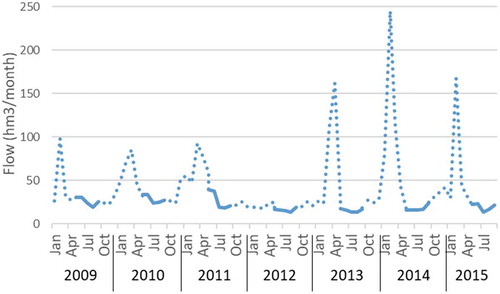
The dry summer season also corresponds to the critical load case. Nearly constant pollutant load combined with low summer flows (due to lower precipitation and higher agricultural abstractions) bring about maximum pollutant concentration.

The available time series is not considered long enough to allow for a temporal sample split for calibration and validation. In our 7-year data sample, putting aside one-third of the data series for validation (Abbaspour et al. 2015) would depopulate an already exiguous calibration period and provide an insufficient calibration period. Previous literature (Daggupati et al. 2015) admits that comparison data are not always available for robust model calibration and validation, requiring additional analysis of model diagnosis to supplement validation and improve confidence in model performance. The implications will be examined in the discussion section.

4 Results

Once the model is set, the coefficients are calibrated to minimize the goal function described in the methodology.

4.1 Water quality model calibration

The model calibrates the applied diffuse load for each area that best fits the observed data. The results show up to 4.8 kg/ha per year loads for nitrate and up to 3.6 kg/ha per year for phosphate, which is consistent with the values in previous literature (Pieterse et al. 2003, Elrashidi et al. 2004, Grizzetti et al. 2008, Yang and Wang 2010). Figure 5 shows the spatial distribution of the calibrated loads.

Figure 5. Nitrate and phosphate calibrated diffuse load.

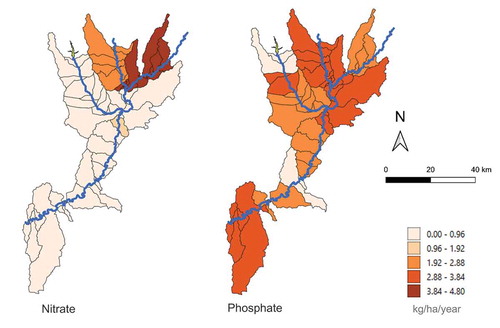
The results suggest a more intense nitrogen fertilization in the Henares River and the Upper Middle Jarama, while phosphorus diffuse pollution appears to be more evenly spread.

Evolution coefficients for the chemical reactions in the river are also assessed. Figure 6 shows the comparison between observed and simulated values.

Figure 6. Simulated vs. observed nutrient values along the Jarama (J.05–J.84) and Tagus (T.00–T.69) rivers.

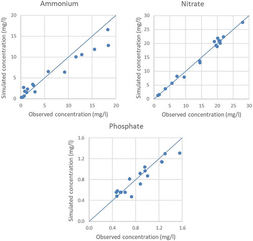
According to Moriasi et al. (2007) for monthly nitrogen and phosphorus predictions, a PBIAS value below 25% is considered “very good”; below 40% is considered “good”; and below 70% is “satisfactory”. Table 2 lists the average PBIAS value for each compound, showing a very good fit for phosphates and nitrates, and an acceptable fit for ammonium. In the absence of validation, Daggupati et al. (2015) recommend to supplement the analysis with a graphical and statistical comparison of model responses at multiple locations. Figure 6 shows that the simulated values follow adequately the observed values when their statistical variation is taken into account. Further confidence on model performance can be gained with scatterplots (Fig. 7), as recommended by Moriasi et al. (2015) for short periods and coarse temporal resolution of available data.

Table 2. Average percentage bias of modelled pollutants.

NO3	NH4	PO4
5.6	42.1	13.1

Figure 7. Scatterplots of observed and simulated concentrations of ammonium, nitrate and phosphate in the study area.

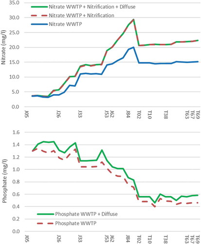
4.2 Relative weight of applied pressures

With this information, we can now calculate the relative weight of each pressure on the receiving waters (Fig. 8). The results show that in the Middle Tagus 68% of the nitrates correspond to direct nitrate discharge from WWTPs, 31% correspond to nitrified ammonium from WWTPs and the remaining 1% corresponds to nitrate from diffuse pollution. In the case of phosphate, 84% corresponds to WWTP effluent and the remaining 16% to diffuse pollution.

Figure 8. Relative weight of pressures on receiving waters, along the Jarama (J.05–J.84) and Tagus (T.00–T.69) rivers.

4.3 Scenarios

We now focus on policy actions needed to achieve a good status in the rivers of the study area.

Since WWTPs are the major contributors to physicochemical pollution, policy intervention should focus on the adaptation of discharge permits. Previous literature on wastewater management optimization (Wang and Jamieson 2002, Zeferino et al. 2017) focuses on site selection and load allocation for new infrastructure. In our case, the site and volume allocation of existing WWTPs will be respected to avoid changes in sewage conduction network. Using the calibrated model, pollutant concentration loads are reduced until the receiving waters achieve the required physicochemical standards. The resulting limits are listed in Table 3.

Table 3. Proposed concentration limits for WWTP effluent permits.

WWTP discharging to	NH4(mg/L)	NO3(mg/L)	PO4(mg/L)
Henares	4.00	60	0.65
Manzanares	0.65	30	0.55
Jarama upstream of Henares confluence	1.00	50	0.55
Jarama downstream of Henares confluence	8.00	60	1.00

A second scenario is built to quantify the effect of the Tagus Segura water transfer on the quality of water with the current WWTP effluent properties. More water diversion from Tagus headwaters (Fig. 1) means that less water is available in the Tagus River to dilute the polluted flows from the Jarama River, resulting in a worse water quality between Aranjuez and Toledo.

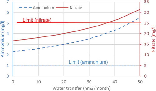
Figure 9 shows that, for an average month, nitrate concentration in the Tagus River between those two cities respects the 25 mg/L limit only when the transferred volume is below 37 hm³/month. Under current circumstances, the ammonium concentration in the same stretch of the Tagus River is above the allowed limit (1 mg/L) for any volume of transferred water.

Figure 9. Simulated effect of Tagus Segura water transfer on nitrate and ammonium concentrations in the Tagus River between Aranjuez and Toledo (T.0–T.64).

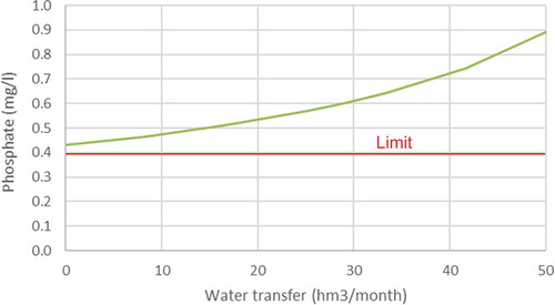
In the case of the phosphate, Fig. 10 shows that the good physicochemical status (when concentration is below 0.4 mg/L of phosphate) is not attained even for small volumes of water transfer.

Figure 10. Simulated effect of Tagus Segura water transfer on phosphate concentration in the Tagus River between Aranjuez and Toledo (T.0–T.64).

Therefore, even in the absence of water transfer, a corrective action is needed in the WWTPs of the Manzanares and Jarama basin in order to achieve a good status for the Tagus River after the confluence with the Jarama River.

Given the large investments associated with the upgrade of the WWTPs and the practical unfeasibility of building all the required infrastructure at the same time, a third scenario is built to define the optimal sequencing for these interventions. In the case of European legislation, preamble 29 of the WFD accepts a “phase implementation of the programme of measures in order to spread the costs of implementation”.

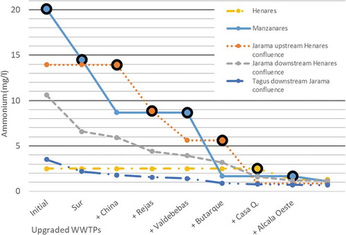
In this phased implementation we propose to focus each time on the river stretch that is the furthest from the physicochemical conditions associated to the good status. That is, to bridge the biggest breach of compliance at each phase. Figure 11 shows the maximum concentration of ammonium for each river stretch. At the initial (current) situation, maximum ammonium concentration (20 mg/L) occurs in the Manzanares River. Initial corrective action is therefore directed to the WWTP discharging the maximum quantity of ammonium in this river, namely Sur WWTP (see Table 1). Once that WWTP is upgraded in line with Table 3 requirements, maximum ammonium concentration (14.5 mg/L) still occurs in the Manzanares River, pointing to the next WWTP in the same river stretch. After the second upgrade, ammonium concentration at Manzanares River drops below 9 mg/L and Jarama River upstream of Henares confluence becomes the critical river stretch with a concentration of 14 mg/L of ammonium. Corrective action therefore addresses the largest pressure on the river stretch, namely effluents from the Rejas WWTP (Table 1). The sequencing of the upgrade of wastewater treatment infrastructure is therefore established until all the receiving surface water bodies reach physicochemical conditions compatible with good status, or until a corrective action would imply disproportionate costs as described in Article 4 of the WFD.

Figure 11. Simulated maximum ammonium concentration per river stretch. The x-axis indicates the initial (current) situation and the upgrade of each WWTP. For Tagus, current levels of transferred volumes are assumed. Black circles represent the most critical position at each stage (requiring priority of intervention).

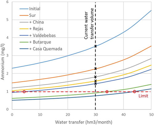
As noted earlier, even in the absence of water transfers, ammonium concentration at Tagus River between Aranjuez and Toledo remains above the 1 mg/L limit, due to the poor water quality of Jarama River flows. After the upgrade of five WWTPs discharging to Manzanares and Jarama Rivers (Fig. 11), ammonium concentration in the Tagus between Aranjuez and Toledo falls below the 1 mg/L limit. A fourth scenario is built to investigate which is a safe volume of water transfer that can be sustained during the process of WWTP upgrading. For “safe” we mean that it is compatible with the achievement of physicochemical conditions associated with a good status of Tagus River between Aranjuez and Toledo. This is the stretch of our study area that is affected by the water transfer. Figure 12 shows that no amount of water transfer would be consistent with the good status before the upgrading of the first four WWTPs.

Figure 12. Expected ammonium concentration for Tagus waters between Aranjuez and Toledo for different water transfer volumes and WWTP upgrade scenarios. Crosses represent the ammonium concentration for each scenario if current transfer volume is kept, and circles represent maximum transfer volume that is consistent with the allowed concentration of ammonium. No water transfer would be consistent for the first four stages.

This scenario shows the intimate relation between the transferred volumes and the upgrading of WWTPs in the Madrid metropolitan region in order to achieve the good status of the receiving waters. Any decision regarding monthly water transfer volumes should guarantee that the resulting quality in Tagus River downstream of the confluence with Jarama is not jeopardized.

5 Discussion

The methodology chosen (a calibrated water quality stationary model upon which change scenarios are built) is deemed appropriate since it can exploit the available data and provide a better understanding of the processes involved.

Special care has been taken to choose the upper and lower ranges of the parameters to ensure that they are consistent with previous literature (Paredes et al. 2013) and representative of site conditions (Daggupati et al. 2015). Combining expert judgment of acceptable ranges with the empirical calibration allows to exploit all the available information, and in our study area has provided a better goodness of fit than the alternative option of assigning the parameter values in a “physical” manner (Thirel et al. 2015).

The implications of not performing a validation of the calibrated values of the parameters can be explored further. The absence of validation entails a loss of information on the predictive capacity of the model. Nonetheless, with such a short sample, a temporal split of data would have added uncertainty to the simulated values (due to a shorter calibration period) and the validation period would be so short that the results would not be statistically significant.

The fact that the four river water quality and six WWTP effluent observations per year are measured in different days implies that the causality link in the model can only be established for long-term averages. This difference in the sampling process responds to the fact that different departments of the Tagus River Basin Authority collect the data for different purposes (compliance with WFD prescriptions on receiving waters, and with wastewater legislation, respectively), not taking into consideration the possible use of data for modelling. A potential amelioration would be the coordination of sampling campaigns to allow for a pairwise collection of pressures and water status data.

In a study area where some stations consistently produce observations with lower variability than others, the proposed goal function (1) will force model simulated values to better replicate the more reliable stations. Conversely, if all observation stations produce measurements with similar variability then there is no advantage of applying the proposed method and other goal functions (PBIAS, R²) would be more appropriate.

Some additional considerations apply to the results of the study. Under the assumption of stationarity, only the steady state is studied; dynamic effects and particular events such as WWTP overflows due to heavy rains are not covered. A further assumption restricts the study to the critical load case of low-flow summer months. This is driven by the lack of data for the highly variable flow of rainy months. If annual averages were to be considered for the established legal standards, concentration limits at plant effluent could be relaxed. On the other hand, only physicochemical elements (i.e. the pollutants limited in WWTP discharge legislation) are studied.

The usual caveats apply to the results due to the high degree of collinearity between the calibrated factors, making aggregate results relatively more reliable. This applies particularly to the diffuse pollution, where total effect results are more solid than the particular geographical distribution.

Although PBIAS was not used for model calibration, it is still a good indicator of goodness of fit since reference thresholds are available in the literature (Moriasi et al. 2007).

6 Conclusions

The paper illustrates an approach for formulating policy recommendations to recover river water quality in a context of scarce observational data. A calibration function for the water quality model is proposed to exploit the statistical properties of the available data. This affords satisfactory calibration results even without a set of event-to-event, pressure-effect data, which would be necessary for a calibration based on R² or Nash-Sutcliffe criteria. As a result, the model replicates the water quality behaviour in the study area with an acceptable degree of certainty.

The approach is applied to the Middle Tagus Basin, where the model is able to quantify the relative weight of the existing pressures on surface water quality, and the policy actions required to achieve a good physicochemical status of surface water bodies. Results show that contaminant loads from WWTPs represent more than 95% of nitrogen pollution and more than 80% of phosphorus pollution. More stringent concentration limits should be set for WWTP effluents. The model determines that ammonium concentration must be below 0.65 mg/L for WWTPs discharging to Manzanares and below 1 mg/L for WWTPs discharging to Jarama upstream of the confluence with Henares.

Due to the magnitude and cost of the intervention, this process should be phased. At each step, the model identifies the river stretch with the largest breach of the pollutant concentration limits and supports the definition of the optimal sequencing of the upgrade of five WWTPs in the study area.

Additionally, the model quantifies the effect of the Tagus Segura transfer in terms of water quality. The expected concentration of physicochemical pollutants is calculated for different transfer volume scenarios. An important result is that with the current sewage treatment infrastructure, Tagus River waters between Aranjuez and Toledo (downstream of the Region of Madrid) cannot attain a good status even in the absence of abstractions in the headwaters for inter-basin transfers.

After the upgrade of WWTP infrastructure, the model is able to inform water authorities on the volume of water that can be transferred without jeopardizing the physicochemical conditions in the Middle Tagus River. Further investigation should focus on the quantification of the costs of the required intervention, and the assessment of their affordability and proportionality with respect to the expected environmental benefits.

Disclosure statement

No potential conflict of interest was reported by the authors.

Supplementary material

Supplemental data for this article can be accessed here.

References

- Abbaspour, K.C., et al., 2015. A continental-scale hydrology and water quality model for Europe: calibration and uncertainty of a high-resolution large-scale SWAT model. Journal of Hydrology, 524, 733–752. doi:10.1016/j.jhydrol.2015.03.027.
- AEMET, 2018. Standard climate values: Madrid, Retiro [ online]. Available from: http://www.aemet.es/en/serviciosclimaticos/datosclimatologicos/valoresclimatologicos?l=3195&k=mad [Accessed 25 June 2019].
- Allaoui, M., et al., 2015. Good practices for regulating wastewater treatment. Legislations, policies and standards. Nairobi, Kenya: United Nations Environment Programme.
- Chapra, S.C., 2008. Surface water-quality modeling. Long Grove, IL: Waveland Press.
- CHT (Confederación Hidrografica del Tajo), 2015a. Anejo 3 de la Memoria. Usos y Demandas De Agua. Plan hidrológico de cuenca [ online]. Available from: http://www.chtajo.es/LaCuenca/Planes/PlanHidrologico/Planif_2015-2021/Documents/PlanTajo/PHT2015-An03.pdf [Accessed 26 June 2019].
- CHT (Confederación Hidrografica del Tajo), 2015b. Anejo 6 de la Memoria. Asignación y reserva de recursos. Plan hidrológico de cuenca [ online]. Available from: http://www.chtajo.es/LaCuenca/Planes/PlanHidrologico/Planif_2015-2021/Documents/PlanTajo/PHT2015-An06.pdf [Accessed 26 June 2019].
- CHT (Confederación Hidrografica del Tajo), 2018. Resultados/informes: aguas superficiales - control fisicoquímico [ online]. Available from: http://www.chtajo.es/LaCuenca/CalidadAgua/Resultados_Informes/Paginas/RISupFisicoQuímico.aspx [Accessed 24 May 2018].
- Cohn, T.A., et al., 1989. Estimating constituent loads. Water Resources Research, 25 (5), 937–942. doi:10.1029/WR025i005p00937.
- Council of the European Communities, 1991. Council directive of 21 May 1991 concerning urban waste water treatment (91/271/EEC). OJ, L 135, 30.5.1991, p. 40–52.
- Cubillo, F., Rodriguez, B., and Barnwell, T.O., 1992. A system for control of river water quality for the community of Madrid using QUAL2E. Water Science and Technology, 26 (7–8), 1867–1873. doi:10.2166/wst.1992.0631.
- Daggupati, P., et al., 2015. A recommended calibration and validation strategy for hydrologic and water quality models. Transactions of the ASABE, 58 (6), 1705–1719.
- De Oliveira, L.M., Maillard, P., and De Andrade Pinto, É.J., 2016. Modeling the effect of land use/Land cover on nitrogen, phosphorous and dissolved oxygen loads in the Velhas River using the concept of exclusive contribution area. Environmental Monitoring and Assessment, 188, 333. doi:10.1007/s10661-016-5323-2.
- DGA (Dirección General del Agua), 2017. Informe de seguimiento de la directiva 91/676 contaminación del agua por nitratos utilizados en la agricultura cuatrienio 2012–2015.
- Di Baldassarre, G., et al., 2013. Towards understanding the dynamic behaviour of floodplains as human-water systems. Hydrology and Earth System Sciences, 17, 3235–3244. doi:10.5194/hess-17-3235-2013.
- Dodds, W. and Smith, V., 2016. Nitrogen, phosphorus, and eutrophication in streams. Inland Waters, 6 (2), 155–164. doi:10.5268/IW.
- Donigian, A.S., 2002. Watershed model calibration and validation: the HSPF experience. Proceedings of the water environment federation. doi:10.2175/193864702785071796.
- Durán Montejano, L., 2016. A comprehensive assessment of precipitation at Sierra de Guadarrama through observation and modeling. Madrid: Universidad Complutense de Madrid.
- Elrashidi, M.A., et al., 2004. A technique to estimate nitrate-nitrogen loss by runoff and leaching for agricultural land, Lancaster county, Nebraska. Communications in Soil Science and Plant Analysis, 35 (17–18), 2593–2615. doi:10.1081/LCSS-200030396.
- Elshemy, M., et al., 2016. Hydrodynamic and water quality modeling of Lake Manzala (Egypt) under data scarcity. Environmental Earth Sciences, 75 (19), 1329. doi:10.1007/s12665-016-6136-x.
- Epelde, A.M., et al., 2015. Application of the SWAT model to assess the impact of changes in agricultural management practices on water quality. Hydrological Sciences Journal, 1–19. doi:10.1080/02626667.2014.967692.
- European Parliament and Council, 2000. Directive 2000/60/EC of the European Parliament and of the council of 23 October 2000 establishing a framework for community action in the field of water policy. OJ, L 327, 2014–7001.
- Fonseca, A., et al., 2014. Integrated hydrological and water quality model for river management: a case study on Lena River. Science of the Total Environment, 485–486 (1), 474–489. doi:10.1016/j.scitotenv.2014.03.111.
- García-Serrano, P., et al., 2009. Guía práctica de la fertilización racional de los cultivos en España. Madrid: Ministerio de Medio Ambiente y Medio Rural y Marino.
- Genkai-Kato, M. and Carpenter, S.R., 2005. Eutrophication due to phosphorus recycling in relation to lake morphometry, temperature, and macrophytes. Ecology, 86 (1), 210–219. doi:10.1890/03-0545.
- Grizzetti, B., Bouraoui, F., and De Marsily, G., 2008. Assessing nitrogen pressures on European surface water. Global Biogeochemical Cycles, 22 (4), n/a–n/a. doi:10.1029/2007GB003085.
- Hutchins, M.G. and Bowes, M.J., 2018. Balancing water demand needs with protection of river water quality by minimising stream residence time: an example from the Thames, UK. Water Resources Management, 32 (7), 2561–2568. doi:10.1007/s11269-018-1946-0.
- IGN (Instituto Geográfico Nacional), 2018. Centro de Descargas del CNIG (IGN) [ online]. Available from: http://centrodedescargas.cnig.es/CentroDescargas/index.jsp [Accessed 24 May 2018].
- INE, 2018. Cifras oficiales de población resultantes de la revisión del Padrón municipal [ online]. Available from: https://www.ine.es/jaxiT3/Tabla.htm?t=2881&L=0 [Accessed 7 April 2019].
- Keupers, I. and Willems, P., 2017. Development and testing of a fast conceptual river water quality model. Water Research, 113, 62–71. doi:10.1016/j.watres.2017.01.054.
- Kottek, M., et al., 2006. World map of the Köppen-Geiger climate classification updated. Meteorologische Zeitschrift, 15 (3), 259–263. doi:10.1127/0941-2948/2006/0130.
- Legates, D.R. and McCabe, G.J., 1999. Evaluating the use of ‘goodness-of-fit’ measures in hydrologic and hydroclimatic model validation. Water Resources Research, 35 (1), 233–241. doi:10.1029/1998WR900018.
- Macklin, M.G. and Lewin, J., 2015. The rivers of civilization. Quaternary Science Reviews, 114, 228–244. doi:10.1016/j.quascirev.2015.02.004.
- MAPAMA (Ministerio De Agricultura Alimentacion y Medio Ambiente). 2014. Real Decreto 773/2014, de 12 de septiembre, por el que se aprueban diversas normas reguladoras del trasvase por el acueducto Tajo-Segura. Boletin Oficial Del Estado, num. 223, 71634–71639.
- MAPAMA (Ministerio de Agricultura Alimentación y Medio Ambiente), 2018. Redes de seguimiento [ online]. Available from: https://sig.mapama.gob.es/redes-seguimiento/ [Accessed 26 June 2019].
- Momblanch, A., et al., 2015. Managing water quality under drought conditions in the Llobregat River Basin. Science of the Total Environment, 503–504, 300–318. doi:10.1016/j.scitotenv.2014.06.069.
- Morales Gil, A., Rico Amorós, A.M., and Hernández Hernández, M., 2005. El trasvase Tajo-Segura. Observatorio Medioambiental, 8, 73–110.
- Moriasi, D.N., et al., 2007. Model evaluation guidelines for systematic quantification of accuracy in watershed simulations. Transactions of the ASABE, 50 (3), 885–900. doi:10.13031/2013.23153.
- Moriasi, D.N., et al., 2015. Hydrologic and water quality models: key calibration and validation topics. Transactions of the ASABE, 58 (6), 1609–1618.
- Munafò, M., et al., 2005. River pollution from non-point sources: a new simplified method of assessment. Journal of Environmental Management, 77 (2), 93–98. doi:10.1016/j.jenvman.2005.02.016.
- Nash, J.E. and Sutcliffe, J.V., 1970. River flow forecasting through conceptual models part I — a discussion of principles. Journal of Hydrology, 10 (3), 282–290. doi:10.1016/0022-1694(70)90255-6.
- Paredes-Arquiola, J., 2018. Manual técnico del modelo RREA [ online]. Available from: https://aquatool.webs.upv.es/files/manuales/rrea/01_ManualTécnicoModeloRREA_V2.pdf [Accessed 26 June 2019].
- Paredes-Arquiola, J., Andreu, J., and Solera, A., 2010. A decision support system for water quality issues in the Manzanares River (Madrid, Spain). Science of the Total Environment, 408 (12), 2576–2589. doi:10.1016/j.scitotenv.2010.02.037.
- Paredes-Arquiola, J., and Solera, A.S., and Andreu, J., 2013. Modelo gescal para la simulación de la calidad del agua en sistemas de recursos hídricos.
- Pellicer-Martínez, F. and Martínez-Paz, J.M., 2018. Climate change effects on the hydrology of the headwaters of the Tagus River: implications for the management of the Tagus–Segura transfer. Hydrology and Earth System Sciences, 22 (12), 6473–6491. doi:10.5194/hess-22-6473-2018.
- Pieterse, N., Bleuten, W., and Jørgensen, S., 2003. Contribution of point sources and diffuse sources to nitrogen and phosphorus loads in lowland river tributaries. Journal of Hydrology, 271 (1–4), 213–225. doi:10.1016/S0022-1694(02)00350-5.
- QGIS Development Team, 2018. QGIS geographic information system. Open Source Geospatial Foundation Project.
- Romanowicz, R.J., Callies, U., and Young, P.C., 2004. Water quality modelling in rivers with limited observational data: river Elbe case study. In: 2nd International Congress on Environmental Modelling and Software[online]. Osnabrück. Available from: https://scholarsarchive.byu.edu/cgi/viewcontent.cgi?article=3190&context=iemssconference
- San Martín, E., 2011. Un análisis económico de los trasvases de agua intercuencas: el trasvase Tajo-Segura. Madrid: Universidad Nacional de Educación A Distancia.
- Shrestha, N.K., Leta, O.T., and Bauwens, W., 2016. Development of RWQM1-based integrated water quality model in OpenMI with application to the River Zenne, Belgium. Hydrological Sciences Journal, 62 (5), 774–799, doi:10.1080/02626667.2016.1261143.
- Strömqvist, J., et al., 2012. Water and nutrient predictions in ungauged basins: set-up and evaluation of a model at the national scale. Hydrological Sciences Journal, 57 (2), 229–247. doi:10.1080/02626667.2011.637497.
- Tarawneh, E., Bridge, J., and Macdonald, N., 2016. A pre-calibration approach to select optimum inputs for hydrological models in data-scarce regions. Hydrology and Earth System Sciences, 20 (10), 4391–4407. doi:10.5194/hess-20-4391-2016.
- Thirel, G., Andréassian, V., and Perrin, C., 2015. On the need to test hydrological models under changing conditions. Hydrological Sciences Journal, 60 (7–8), 1165–1173. doi:10.1080/02626667.2015.1050027.
- Thomann, R.V. and Mueller, J.A., 1987. Principles of surface water quality modeling and control. New York: HarperCollins.
- Vega, M., et al., 1998. Assessment of seasonal and polluting effects on the quality of river water by exploratory data analysis. Water Research, 32 (12), 3581–3592. doi:10.1016/S0043-1354(98)00138-9.
- Wang, C.G. and Jamieson, D.G., 2002. An objective approach to regional wastewater treatment planning. Water Resources Research, 38, 3. doi:10.1029/2000WR000062.
- Ward, A.D. and Elliot, W.J., 1995. Environmental hydrology. Boca Raton, FL: Lewis Publishers.
- Wellen, C., et al., 2014. Application of the SPARROW model in watersheds with limited information: a Bayesian assessment of the model uncertainty and the value of additional monitoring. Hydrological Processes, 28 (3), 1260–1283. doi:10.1002/hyp.v28.3.
- Xue, C., Yin, H., and Xie, M., 2015. Development of integrated catchment and water quality model for urban rivers. Journal of Hydrodynamics, Series B, 27 (4), 593–603. doi:10.1016/S1001-6058(15)60521-2.
- Yang, Y.S. and Wang, L., 2010. A review of modelling tools for implementation of the EU Water Framework Directive in handling diffuse water pollution. Water Resources Management, 24 (9), 1819–1843. doi:10.1007/s11269-009-9526-y.
- Zeferino, J.A., Cunha, M.C., and Antunes, A.P., 2017. Adapted optimization model for planning regional wastewater systems: case study. Water Science and Technology, 76 (5), 1196–1205. doi:10.2166/wst.2017.302.
- Zhang, H. and Huang, G.H., 2011. Assessment of non-point source pollution using a spatial multicriteria analysis approach. Ecological Modelling, 222 (2), 313–321. doi:10.1016/j.ecolmodel.2009.12.011.
- Zhao, G.J., et al., 2010. Development and application of a nitrogen simulation model in a data scarce catchment in South China. Agricultural Water Management, 98, 619–631. doi:10.1016/j.agwat.2010.10.022.
- Zou, R., et al., 2014. Uncertainty-based analysis on water quality response to water diversions for Lake Chenghai: a multiple-pattern inverse modeling approach. Journal of Hydrology, 514, 1–14. doi:10.1016/j.jhydrol.2014.03.069.