Improving flood forecasting using an input correction method in urban models in poorly gauged areas

ABSTRACT

Poorly monitored catchments could pose a challenge in the provision of accurate flood predictions by hydrological models, especially in urbanized areas subject to heavy rainfall events. Data assimilation techniques have been widely used in hydraulic and hydrological models for model updating (typically updating model states) to provide a more reliable prediction. However, in the case of nonlinear systems, such procedures are quite complex and time-consuming, making them unsuitable for real-time forecasting. In this study, we present a data assimilation procedure, which corrects the uncertain inputs (rainfall), rather than states, of an urban catchment model by assimilating water-level data. Five rainfall correction methods are proposed and their effectiveness is explored under different scenarios for assimilating data from one or multiple sensors. The methodology is adopted in the city of São Carlos, Brazil. The results show a significant improvement in the simulation accuracy.

KEYWORDS:

• data assimilation
• semi-distributed model
• flood modelling
• physically-based model
• SWMM

Editor A. CastellarinAssociate editor A. Efstratiadis

1 Introduction and scope

Intense urban growth without proper management and adequate drainage systems, along with the effects of increasing weather variability and climate change, are the main causes of urban flood aggravation in cities, especially in small catchments (Tollan 2002, Ashley et al. 2005, Bai et al. 2018). Additionally, the measurements of rainfall in many cities are scattered and not very accurate, and this is a major challenge for modelling and predicting floods in a timely manner for decision makers.

In response, many research studies have investigated how to improve flood forecasting. Among the approaches used are data assimilation (DA) techniques, which have become widely used to improve hydrological predictions, updating the model as a response to real-time observations (Young 2002, Hutton et al. 2012, He et al. 2017, Mazzoleni et al. 2018a). The main idea of most data assimilation methods is to quantify errors in field data and in simulations to update the hydrological states optimally, ensuring minimization of simulation error (Collier 2007, Coustau et al. 2013, McMillan et al. 2013, Thiboult and Anctil 2015). The updates can be made in the inputs, parameters and states of hydrometeorological models (Refsgaard 1997, Liu and Gupta 2007, Seo et al. 2009).

Kalman filter (KF) is the most widely known DA method; however, it is optimal only for linear processes (Maybeck 1982, Walker and Houser 2005). To account for nonlinear systems, several variations such as the particle filter (Moradkhani et al. 2005, Andrieu et al. 2010, Moradkhani et al. 2012), extended Kalman filter (Francois et al. 2003) and the ensemble Kalman filter (Reichle et al. 2002, McMillan et al. 2011, Mazzoleni et al. 2018b) have been proposed; the latter is the most used technique in Earth sciences (Evensen 2003, Chen et al. 2013). Although these methods are designed for nonlinear models, they use linearization during the update process (Liu et al. 2012).

A number of authors have explored the use of data assimilation methods to update urban models. For instance, Hutton et al. (2014) developed a methodology employing a deterministic Kalman filter to update the states of an urban model as a response to downstream observations. Their results show improvements in the discharge forecasts. However, the presence of threshold system behaviour in controlled urban systems affects ability of the DA procedure, resulting in de-coupling of the downstream catchment response to changes in upstream behaviour. Hansen et al. (2014) used DA for the distributed hydrodynamic urban drainage model MIKE URBAN. The updating process was carried out in a deterministic manner and demonstrated improvements in the simulations, despite the fact that the uncertainties of the model structure and observational data were not considered. Borup et al. (2018) tested the use of ensemble Kalman filter for the MIKE URBAN model in an experiment to evaluate the possibility of using constant Kalman gain updating to address the problem of high computational demand when the ensemble is calculated in real time. Their results showed that the gain is nonlinear and varies greatly in time, requiring the use of the complete ensemble Kalman filter scheme.

In fact, just a few studies have investigated the use of DA approaches for real-time monitoring in small urban catchments subject to flash floods (Xie and Zhang 2010, Chen et al. 2013). In contrast to large or medium-scale basins, small urban catchments may be affected by intense local precipitation (WMO 2011), which, combined with increased runoff by urbanization, requires faster responses from hydrological models to ensure their utility for flood forecasting (Yang et al. 2011, Chen et al. 2013, Yin et al. 2016). Furthermore, urban models are highly nonlinear with many physical state variables and, consequently, computationally costly, posing a further challenge for their real-time updating (Hansen et al. 2014, Borup et al. 2018).

Rainfall estimation has the fundamental role to perform streamflow simulations in hydrological models. This is especially vivid when the quantity and intensity of rainfall vary depending on previous conditions (Harader et al. 2012), and in urban areas where runoff is usually extremely sensitive to the spatial distribution of rainfall, and the flood responses are caused by spatially localized convective precipitation (Zawadzki 1973, Segond et al. 2007). Furthermore, a study performed by McMillan et al. (2011) showed that, for heavy rainfall events, hydrological models have high multiplicative errors. The result is that uncertainty in rainfall measurement and forecasting leads to errors in flow forecasts, even if real-time hydrological models are well-calibrated (Pedersen et al. 2016). An option to address this could be the use of DA schemes for updating the rainfall inputs (rather than model states) as a response to observed water levels or flow data. However, quite surprisingly, only a few studies have proposed and explored this possibility (Kahl et al. 2008, Stanzel et al. 2008, Divac et al. 2009, Harader et al. 2012), and none of the mentioned examples was developed for application in urban catchments. Furthermore, we could not find reported research on DA methods aiming to correct rainfall inputs based on observed water levels for urban models.

Analysis of the literature and known practice leads us to conclude that data assimilation in physically-based models for basins with short lead time, and the inaccuracies in rainfall inputs, are important issues to be investigated for flood forecasting and monitoring in urban systems. Therefore, the main objectives of this study are: (a) to analyse the hydrological model sensitivity to input variation (precipitation); (b) to propose a new variant of DA methodology that corrects the model input using observed water levels from in situ sensors; and (c) to assess the effect of the number and location of water-level sensors (used to correct model input) on model accuracy. The methodology is tested in a case study in the Monjolinho catchment, located in the city of São Carlos, São Paulo State, Brazil, modelled by the Storm Water Management Model (SWMM) (Rossman 2010).

2 Case study and datasets

2.1 Monjolinho catchment and its flood history

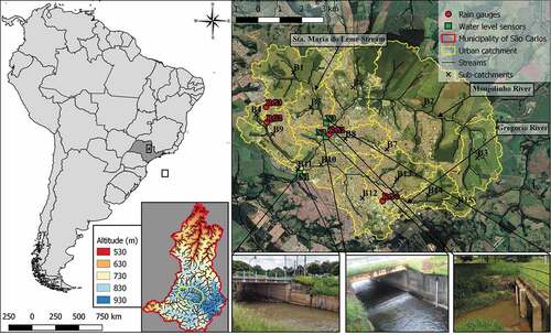
The case study is located in the Monjolinho catchment (Fig. 1), located in São Carlos, state of São Paulo, Brazil. The total area of the municipality of São Carlos (Fig. 1, zoom map on the left) is about 1136.91 km². The population density of the city is about 194.53 inhabitants/km² and the total population is estimated as 249 415 inhabitants (IBGE 2018). The average altitude is about 856 m a.s.l., and the soil is highly permeable. The Monjolinho River starts in the southeast of São Carlos, crossing the entire urban area of the city, with an approximate altitude of 900 m a.s.l. The total area of the Monjolinho catchment is 209.16 km². For this study, the urban portion of the Monjolinho catchment was delimited (Fig. 1, map on the right), resulting in an area of about 79.6 km². The springs of the catchment are located within the municipality of São Carlos to the east, and its valley topographically delimits the urban core of the city. Hence, any information from upstream of the delimited area is not considered in the modelling procedure.

Figure 1. Monjolinho catchment in the city of São Carlos, São Paulo State, Brazil. The photographs at the bottom right show the three water–level monitoring locations N1, N2 and N3 (left to right).

The city has a long history of flooding. Mendes and Mendiondo (2007) estimated, based on historical data from 1940 to 2004, that the average return period of flood occurrence is 0.65 events/year with a standard deviation of 0.84. Their study also showed that the cumulative number of flood occurrences increased with the catchment urbanization. This historical data suggests that there is a clear need to adopt structural and non-structural means for the containment of floods, but the proposals to solve the problem recorded in official documents are very onerous and have not yet been adopted. (Barros et al. 2007). Despite the high frequency of floods, there is neither systematized flood data nor early warning system for São Carlos.

2.2 Datasets

2.2.1 Water-level data

Data from three monitoring locations (sensors N1, N2 and N3) are used; these sensors collect water-level data every 15 min (Fig. 1). Sensor N1 is installed in the outlet of the catchment delimited for this study and in the Monjolinho River. It is in a constructed canal without margin conservation. The riverbank has just a 2 m wide strip of grass coverage. The area receives a significant contribution of surface runoff from the drainage on the left side of the catchment along the Gregorio River, and frequent fluvial floods occur there. The second location (N2) is in the Monjolinho River after it has received the contribution from Santa Maria do Leme Stream. At this location, the canal is constructed from cement; this location is also in an urbanized area of the city and has a strip of around 2 m of grass followed by asphalt. Sensor N2 is installed upstream of sensor N1 and its area does not suffer from flooding. Sensor N3 is installed in a section of the Santa Maria do Leme Stream near the junction with the Monjolinho River and upstream of the other monitoring locations. The river has a natural bed, which is quite silted at this location due to the lack of native vegetation and protected area on the banks of the stream. Along this section, the environment consists of approximately 2 m of grass, followed by asphalt and an area of intense urbanization. Due to these characteristics, canal overflows are often observed.

2.2.2 Rainfall data

The input data come from the four raingauges shown in Fig. 1 (RG1–RG4), at 15-min intervals. To generate the spatially distributed rainfall field, we used the inverse distance weighting (IDW) method to interpolate point data from the four raingauge stations and estimate the mean spatial rainfall for each sub-catchment.

3 Methodology

3.1 Hydrological urban modelling

The SWMM (Rossman 2010) is a modelling system with integrated hydrological and hydraulic modelling modules, which is capable of simulating single events or long-term simulations of runoff in urban catchments with pipe and open flow networks. The hydrological module simulates the sub-catchment behaviour, including an internal infiltration module. The rainfall–runoff component is lumped and conceptual at the sub-catchment scale. A sub-catchment can be defined by the user and is divided into pervious and impervious portions. Each part is modelled as a nonlinear reservoir with a capacity given to the maximum depression storage. The hydraulic module propagates the surface runoff, coming from the hydrological model, along rivers, canals and other conduits.

The input of the hydrological model are width, average slope and infiltration, Manning’s coefficient for pervious and impervious area, percentage of impervious area with no depression storage, depth of depression storage on pervious and impervious areas and the percentage of impervious area. For the hydraulic module, the main inputs are the canal roughness.

We developed an automatic calibration tool for SWMM using genetic algorithms (GA) as the optimization technique; this is written in Python 3.6. We used the distributed evolutionary algorithms in Python (DEAP) as a framework for the GA optimization (Fortin et al. 2012) and the SWMM5 library for the SWMM calling interface developed by Pathirana (2015).

In our study, we calibrated the SWMM model using water-level values instead of flow data, as the rating curve was not available. This decision was based on the study by Lindström (2016), who showed good results for hydrological model calibration using observed water-level data instead of observed discharge or establishing a rating curve. The study by Lindström (2016) also proposes efficiency evaluation equations for data from multiple water-level stations, such as the spatial Nash-Sutcliffe efficiency, SPATNSE (Equation (1)). The maximization of SPATNSE was set as the objective function in the calibration tool developed.

(1a) $\mathrm{S}\mathrm{P}\mathrm{A}\mathrm{T}\mathrm{N}\mathrm{S}\mathrm{E}=1-\frac{{\sum }_{j=1}^K{\left({\bar{H}}_j^{\ast }-{\bar{H}}_j\right)}^2}{{\sum }_{j=1}^K{\left({\bar{H}}_j-\frac{1}{K}{\sum }_{j=1}^K{\bar{H}}_j\right)}^2}$(1a)

(1b) ${\bar{H}}_j^{\ast }=\left({H^{\ast }}_{j_i}:i=\left[1,c_j\right]\right)=\frac{1}{c_j}{\sum }_i{H}^{\ast }{{ }_j}_i$(1b)

(1c) ${\bar{H}}_j=\left(H_{j_i}:i=\left[1,c_j\right]\right)=\frac{1}{c_j}{\sum }_i{H_j}_i$(1c)

where $H_{j_i}^{\ast }$ are the simulated values for the jth station at time step i, $\left[1,K\right]=\left\{j\in \mathbb{N}:1\le j\le K\right\}$, $H_{j_i}$ are the observed values for the jth station at time step $i$, ${\bar{H}}_j^{\ast }$ is the average value of $H_j^{\ast }$ for the jth station, ${\bar{H}}_j$ is the average value of $H_j$ for the jth station, $c_j$ is the number of values in the time series for station j, i is the index of time steps with observations in a time series of a station, j is the index of stations, and K is the total number of stations. The simulated and observed variables are water levels at sensor locations. The value of SPATNSE ranges between $-\mathrm{\infty }$ and 1.

3.2 Model set-up

The basin is delineated into 15 sub-catchments and modelled using the SWMM. For the model routing, we set the dynamic wave equations, and for the infiltration module in SWMM, we opted for the SCS curve number (CN) method. This infiltration method is an approach adapted for the CN of the NRCS (Natural Resources Conservation Service of the US Department of Agriculture) to estimate the runoff (Cronshey 1986). Originally, the method combines losses due to interception, depression storage and infiltration to predict the total rainfall excess. In SWMM, the CN method is used to compute only the infiltration losses. The surface runoff is calculated using a nonlinear reservoir model and by applying the Manning equation to calculate the flow rate. The depression storage is not linked to the infiltration method, giving more freedom for the modeller to choose the value for the Manning parameter. The moisture retention capacity of the soil (S) is reduces during wet periods by the infiltration volume and increases during dry periods by a first-order recovery model. Then, the current value of S is used when the next rainfall event starts allowing the model to calculate infiltration as a function of cumulative rainfall volume. More details about the modified CN method can be found in Rossman and Huber (2016).

Eight rainfall events between November 2013 and April 2014 are used for calibration and validation. The events are split into three subsets according to the average intensity of the rainfall: light, moderate and heavy. Then, the events are chosen at random for two groups: for calibration and validation – with the restriction of at least one event of each subset for each group. The GA approach is used for calibration, considering the following set-up: two-point crossover, flip-bit mutation algorithm, selection by tournament, 80% crossover probability, 5% mutation probability and initial population size of 300 individuals. Model calibration resulted in a SPATNSE value of 0.63 for the calibration period and 0.61 for the validation period. Table 1 presents the events selected.

Table 1. Total rainfall measured by the raingauges RG1–RG4 and the peak water level measured by sensors at monitoring locations N1, N2 and N3 during the events used for calibration and validation of the model.

Event	Date(dd/mm/yyyy)	Duration (h)				Total rainfall (mm)				Peak water level
		RG1	RG2	RG3	RG4	RG1	RG2	RG3	RG4	N 1	N2	N3
Calibration
1	05/11/2013	08:45	04:40	08:55	08:55	9.6	12.2	10.0	8.2	0.74	0.48	0.93
2	06/11/2013	09:40	10:00	09:45	10:35	45.2	40.4	37.8	48.2	1.19	1.03	1.43
3	24/11/2013	00:50	00:55	01:00	01:20	16.6	6.6	10.8	19.4	0.81	0.57	1.11
4	13/04/2014	01:00	01:40	01:05	00:10	26.8	25.2	38.0	0.8	2.44	2.28	-
Validation
1	04/11/2013	04:40	04:35	05:05	16:10	64.6	47.4	41.6	73.8	2.00	1.56	4.02
2	07/11/2013	03:20	03:05	00:10	02:55	9.6	2.4	1.6	5.6	0.67	0.48	1.05
3	16/11/2013	01:15	01:25	00:35	01:20	10.6	5.6	5.2	16.4	0.79	0.49	1.84
4	10/12/2013	03:15	01:30	-	01:10	13.4	9.6	-	5.2	1.25	1.22	1.51

3.3 Data assimilation framework

Based on the description by Rossman and Huber (2016), SWMM is a distributed discrete time simulation model that computes new values of its state variables over a sequence of time steps. At each time step, the system is subject to a new set of external inputs. SWMM state variables in the runoff, infiltration and flow routing processes are: depth of runoff on sub-catchment surface, cumulative excess infiltration volume, upper zone moisture content, time until the next rainfall event, cumulative rainfall for current event, soil moisture capacity remaining, depth of water at a node, flow rate in a link and flow area in a link. The relationship between the state variables of the SWMM model and observations is not linear, which means that the observations cannot be mapped directly in the state space. In addition, in order to speedily provide results for real-time operation for urban basins subject to flash floods, the assimilation procedure must provide reliable results within a short computational time. To account for that, in this paper we propose an approach to correct the model inputs as a response to hourly real-time observed water-level data from different in situ sensors. The method is designed to dynamically assimilate water-level information from one to multiple sensors simultaneously. The general methodology is outlined in Fig. 2. Note that the proposed method does not take into account the uncertainty of the model parameters and water-level observations, an option which it is planned to implement in a forthcoming version of this method.

Figure 2. Flowchart of the data assimilation methodology.

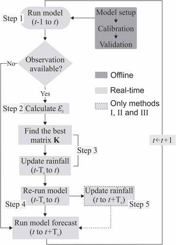
In the first step, SWMM simulation is run with the estimated rainfall values as input until time step $t$, which is the moment when the water-level observation $H_t$ becomes available.

In the second step, $H_t$ is compared to the corresponding simulated water level ($H_t^{\ast }$) for the same location, and the squared error between the model simulation and the observation is calculated (Fig. 3(a)). It is worth noting that there is a possibility of receiving observational data from more than one location simultaneously. In such a case, the error ${\epsilon }_t$ for receiving observed water level at time $t$ at one or more location is calculated by averaging all errors:

(2) ${\epsilon }_t=\frac{1}{N}{\sum }_{j=1}^N{\left(H_{t,j}^{\ast }-H_{t,j}\right)}^2$(2)

Figure 3. Data assimilation with input rainfall correction: (a) calculating the error ${\epsilon }_t$ when receiving field data; (b) after calculating the error, rainfall is updated by one of the methods (I, II, III, IV or V); and (c) the rainfall correcting process for each sub-catchment. Precipitation data is updated by the inner product of its original values by the optimized coefficients contained in the matrix K (Equation (5)).

where $N$ is the number of locations receiving information at time t, $H_{t,j}$ (m) is the observed water level at the jth node at time t, and $H_{t,j}^{\ast }$ (m) is the simulated value at time t.

Seo et al. (2003) pointed out that the assimilation window must be equivalent to the time of response of the basin so that the memory of the system is reflected in the process of assimilation. Thus, in the third step, the time of concentration ($T_C$) of the catchment is used as the time window for correcting the model input; hence, we assume that the rainfall which occurred before $T_C$ does not affect the river flow at time t. Rainfall values present in the moving assimilation window for all the sub-catchments are corrected by a certain multiplier; in Equation (5) this is expressed as the inner product of the estimated rainfall and a matrix $K$ of coefficients. The values of the matrix corresponding to time step t are estimated in a quasi-optimal way to reduce the error calculated in Step 2; then, they are propagated through the assimilation window – this can be done by several methods. The details of the optimization procedure and the methods to update rainfall are explained in the next sections. The corrected precipitation of the sub-catchments ${\mathit{P}}^{+}$ is a matrix with the same dimensions as the matrix K (Equation (3)) and the rainfall P estimated in the sub-catchments.

(3) $\mathit{K}=\left({\mathit{k}}_{\mathit{i}j}\right)\in {\mathbb{R}}^{m\times n}$(3)

(4) $\mathit{P}=\left({\mathit{p}}_{ij}\right)\in {\mathbb{R}}^{m\times n}$(4)

(5) ${\mathit{P}}^{+}\leftarrow ⟨\mathit{K},P⟩\in {\mathbb{R}}^{m\times n}$(5)

Matrices $\mathit{P}$ and ${\mathit{P}}^{+}$ contain, respectively, the original rainfall and the corrected rainfall values of all sub-catchments (Equations (4)–(5)). Matrices $\mathit{K}$, $\mathit{P}$ and ${\mathit{P}}^{+}$ comprise n arrays of coefficients containing m elements each, where n is the number of sub-catchments and m is defined as the floor value resulting from the division of the $T_C$ by the default time step. The change in rainfall is carried out with the aim to obtain a better simulation not only at the location where the field information is received but, since it is a semi-distributed model, also throughout the basin.

In the fourth step, the model is re-run from time t – $T_C$ to time t with the updated rainfall values. Finally, in Step 5, the coefficients used to change rainfall backwards in time are also applied to correct precipitation forward in time, from time step t to t + $T_C$.

3.4 Optimization method

The real-time DA methodology proposed in this study focuses on urban basins with a rapid response requiring model simulations with short time steps. The quasi-optimum values for the DA coefficients in K need to be found within one such time step, so settings for the DA and optimization algorithms have to take the simulation time constraints into account.

The objective function (OF) to be minimized is the error between the observed and simulated water level when receiving new field data at one or more locations in the catchment (Equation (2)). The decision variables to be identified are the coefficients that change the precipitation values of each sub-catchment at the time step t, which is the moment when field data are received. The first row of the matrix K corresponds to these coefficients (i = 1). Therefore, we use the coefficients vector for the first line of the matrix K, i.e. for an observation received at time t, ${\mathit{k}}_j\leftarrow {\mathit{K}}_{1,j}$.

We use a randomized search by canonical GA set up with the following parameters: two-point crossover, bit-flip mutation algorithm and selection by tournament, 50% crossover probability, 2% mutation probability and initial population size of 100 individuals. The GA evaluates the OF for each new vector of decision variables (minimizing the average water-level error at time t by correcting coefficients and, hence, changed rainfall inputs). This is done by running SWMM from $t-T_C$ to $t$, and recalculating ${\epsilon }_t$ with the new rainfall inputs. Optimization continues until the found solution cannot be improved (or considered acceptable), or until it reaches the 15-min time limit. We adopted an absolute error of 5 cm between the observed and simulated water levels as an acceptable error. In addition, we constrained the decision variables to limit the amount allowed to change rainfall – between – 60% to +60% of the original data. This is done to preserve the characteristics of the rainfall, even considering the uncertainties in its estimation. Based on the this, the optimization problem is formulated as follows:

(6) $\mathrm{O}\mathrm{F}:\mathrm{m}\mathrm{i}\mathrm{n}{\epsilon }_t$(6)

$\mathrm{S}\mathrm{u}\mathrm{b}\mathrm{j}\mathrm{e}\mathrm{c}\mathrm{t}\mathrm{t}\mathrm{o}-0.4\le {\mathit{k}}_j\le 1.6:j\in \left[1,n\right],$

3.5 Model input correction

Five different rainfall correction methods are proposed. The rainfall values are corrected backwards in time using the n coefficient vectors of size m optimized from t to $t-T_C$. In the first three methods (I, II and III in Fig. 3(b)), after finding the quasi-optimal coefficients in the steps going backwards from time step t, the rainfall values are corrected with these same values until t + $T_C$. The other two methods (IV and V in Fig. 3(b)) modify precipitation values only going backwards in time. The influence of methods IV and V for flood prediction is limited to the correction effect of rainfall only up to $T_C$. The methods are as follows:

Method I. Each sub-catchment has a vector ${\mathit{k}}_j$, which decreases according to a linear function (Equation (7b)); the ${\mathit{k}}_j$ value is the maximum at time t and decreases linearly until $t-T_C$, where its value is null. Thus, the change in the rainfall is highest close to the present moment (when receiving information) and progressively decreases to zero going backwards in time. The quasi-optimal coefficient values are used to propagate the rainfall correction also into the future (Fig. 3(b), I), with the same scheme, but going forward in time, with linearly progressively decreasing values (Equation (8c)).

(7a) ${\mathit{k}}_i\leftarrow {\mathit{K}}_{ij}\mathrm{f}\mathrm{o}\mathrm{r}\mathrm{e}\mathrm{a}\mathrm{c}\mathrm{h}j:j\in \left[1,n\right]$(7a)

(7b) ${\mathit{k}}_i=\frac{(-{\mathit{k}}_j+1)}{x}i+{\mathit{k}}_j:i\in \left[1,m\right]$(7b)

(7c) ${\mathit{k}}_i^{\ast }=\frac{\left({\mathit{k}}_j-1\right)}{x}i+1:i\in \left[1,m\right]$(7c)

(8) $x=\left|\frac{t-T_C}{s}\right|$(8)

where ${\mathit{k}}_i$ is the ith coefficient in the changing rainfall vector backwards, ${\mathit{k}}_i^{\ast }$ is the ith coefficient in the changing rainfall vector forward, $m$ is the number of elements in the rainfall input in the window of time between $t$ and $T_C$, and $s$ is the time step size.

Method II. The rainfall is corrected by the ${\mathit{k}}_j$ values going backwards and forwards in time, from $t-T_C$ to $t+T_C$. However, in Method II the coefficient values remain constant, i.e. the same multiplier value is used for all time steps (Fig. 3(b), II).

Method III. In this method, the rainfall is corrected going both backwards and forwards in time. Going backwards, the coefficient values remain constant and going forwards they decrease linearly (Equation (7c), Fig. 3(b), III).

Method IV. This method uses updates similar to Method I: from t back to $t-T_C$ the coefficients decrease linearly (Equation (7b), Fig. 3(b), IV), but do not update forward values.

Method V. Similarly to Method II, the coefficients ${\mathit{k}}_j$ remain constant for backward updating from t to $t-T_C$, but do not update forward values (Fig. 3(b), V).

3.6 Sensitivity analysis

Taking into account that (a) the model used is semi-distributed allowing different rainfall values for each sub-catchment, and (b) the assimilation method aims to identify the (different) correcting coefficients, it is important to know the relative contribution of each sub-catchment to runoff generation when varying the model input. Therefore, the model sensitivity analysis is carried out with rainfall changing for each sub-catchment. The estimated precipitation at each sub-catchment is varied, one at a time, and the effects on the runoff simulation at the outlet are quantified. The data assimilation methods optimize the values considering the coefficients of variation between – 60% and +60%. These same values are used in the sensitivity analysis to vary the original amounts of rainfall, with regular intervals of 30%. Finally, the model output changes corresponding to the rainfall variation of each sub-catchment (indicating the sensitivity) are compared to the model output changes when DA is applied. It is expected that, in relative terms, there should be a certain agreement between the two, showing that the search method followed the physical meaning of rainfall variation. Otherwise, it will indicate that DA is also correcting structural problems of the model.

3.7 Evaluation criteria

To evaluate a change in model performance when DA is employed, the Nash-Sutcliffe efficiency (NSE) index is used (Nash and Sutcliffe 1970):

(9) $\mathrm{N}\mathrm{S}\mathrm{E}=1-\frac{{\sum }_{i=1}^N{\left(H_i-H_i^{\ast }\right)}^2}{{\sum }_{i=1}^N{\left(H_i-{\bar{H}}_i\right)}^2}$(9)

where $H_i$ is the observed water level at time step i; $H_i^{\ast }$ is the simulated water level at time step i; and $N$ is the total number of water-level observations.

4 Experimental set-up

4.1 Assimilating data from one water-level sensor

The usefulness of the data assimilation methodology is evaluated for a catchment with spatially varying characteristics, modelled by a semi-distributed model, and with more than one flood monitoring locations. All this requires us to explore various ways of assimilating measurements in a distributed system. This first experiment aims to assess the effectiveness of DA methods when receiving regular information from only one location. The evaluation is made, accounting for the effects of rainfall updating across all sub-catchments, by assessing the water-level simulations at the location where the sensor data is assimilated as well as at other monitoring locations where the data is not assimilated. Assimilation of water-level data is tested for the three monitoring locations, one at a time, described as scenarios 1, 2 and 3, depending on which sensor provides the data to be assimilated (Table 2). The time step of the model is 15 min and the sensor information is assimilated at regular intervals of 1 h. Five methods of rainfall correction are employed, as described in Section 3.5, and their effectiveness is compared.

Table 2. Scenarios of model input correction at three water-level monitoring locations within the Monjolinho catchment.

Scenario	Location
	N1	N2	N3
1		×
2			×
3	×
4	×	×	×
5	×		×
6	×	×
7		×	×

4.2 Assimilating data from multiple sensors

In this second experiment, we consider the DA scenarios handling water-level information received at the same time from several measurement locations. It is assumed that the observed water-level data arrives synchronously at a frequency of 1 h under assimilation scenarios 4, 5, 6 and 7. Table 2 shows the combination of sensors that provide the data to be assimilated at the same time. For all scenarios, the performance evaluation is done considering the effects of rainfall updating throughout the catchment in the model runs at all the locations monitored by water-level sensors.

5 Results and discussion

5.1 Sensitivity analysis

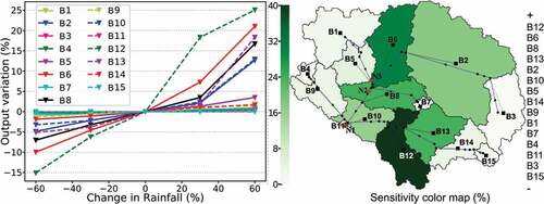
Figure 4 shows the sensitivity analysis results. The graph presents the impact of varying the original rainfall amount in each sub-catchment for the maximum water level at the outlet of the catchment. The results show that an increase in rainfall has a more significant influence on the output than its reduction. The map visualizes the model output sensitivity to rainfall variation over the catchment. The percentages shown for each sub-catchment are the maximum water-level variations at the outlet resulting from variations in rainfall in the range from – 60% to +60% of the original values.

Figure 4. Analysis of model output sensitivity on rainfall variation over the 15 sub-catchments, showing the water-level peak variation (left) and the maximum water-level peak variation (right) when changing the original value from – 60% to +60%, both assessed at the outlet due to changes of rainfall in sub-catchments B1–B15.

Table 3 shows the area, drainage area upstream the outlet, percentage of imperviousness and slope of each sub-catchment, which are all determined in the calibration process. It also shows the time of concentration ($T_C$) and the results of the sensitivity analysis in terms of the percentage of output variation. Romero (2016) determined the $T_C$ values listed in Table 3. He used the same SWMM Monjolinho catchment model structure as used in this paper and applied the Kirpich method to calculate the $T_C$ upstream of each node. The presented catchment characteristics are useful for evaluating the output behaviour. It is worth mentioning, however, that the sensitivity analysis is performed considering only the effect of the rainfall variation at the maximum water level in the outlet of the catchment; we are not accounting for the influence associated with the corresponding area, time of concentration and other parameters, nor their combined effects that also influence the maximum water level during a rainfall event.

Table 3. Model parameter values per sub-catchment and the maximum water-level variation found in the sensitivity analysis. $T_C$ values determined by Romero (2016).

Sub-catchment	Area (km2)	Drainage area upstream (km2)	Imperviousness (%)	Slope (%)	$T_C$ (h)	Maximum water-level variation (%)
B1	7.30	7.30	23.50	5.45	0.23	1.62
B2	21.84	30.59	30.35	10.30	0.54	17.52
B3	8.75	8.75	13.54	11.67	0.41	0.20
B4	0.94	0.94	54.04	7.90	0.38	0.81
B5	3.68	10.98	31.28	8.37	0.30	5.39
B6	7.43	38.02	85.49	9.49	1.66	31.00
B7	0.54	0.54	86.54	7.80	0.13	1.62
B8	4.82	54.36	93.84	8.96	1.89	23.72
B9	4.32	5.26	37.47	8.21	0.49	3.23
B10	3.89	79.44	34.34	8.55	2.13	16.17
B11	0.11	79.55	17.00	12.75	2.13	0.27
B12	6.09	15.93	84.91	9.12	0.99	40.16
B13	5.50	9.84	82.77	11.51	0.56	23.45
B14	3.31	4.34	41.37	9.77	0.54	3.50
B15	1.03	1.03	10.23	9.40	0.23	0.20

The sub-catchments that contribute most to increasing the water-level peak in the outlet are B2, B6, B8, B10, B12 and B13. These sub-catchments have a significant effect on the water level at location N1. Analysing the sensitivity map and the location N2 (Fig. 4, right), we can conclude that the raingauges influencing the water-level variation to this site are B2 and B6, and for P3 they are B1 and B5. Thus, it is evident that the catchments in the upper reaches of the rivers have less influence on the runoff, the probable reason being that the areas around the springs are covered with vegetation and, consequently, they are more permeable. The sub-catchments located in the most urbanized area of the basin are the most sensitive, except for sub-catchment B7. Location and land use are crucial for runoff generation, as well as the catchment area. This last factor is determinant in making sub-catchment B7 less sensitive since its drainage area is the second smallest among the 15 sub-areas, being only 0.54 km².

5.2 Assessing the methods of rainfall correction when assimilating data from a single sensor

Figure 5 shows the NSE for scenarios 1, 2 and 3 when water-level data are received at one location at a time, for the five updating methods (I–V). The NSE values shown in Fig. 5 are the averages across all the rainfall events used in this study, while Table 4 details the NSE values per event.

Table 4. Performance results (NSE) for each rainfall event of the model simulations of water levels and after input correction by methods I–V, when assimilating data from one sensor at a time (scenarios 1, 2 and 3).

No update	N1	N2	N3	N1	N2	N3	N1	N2	N3	N1	N2	N3
	Event 1			Event 2			Event 3			Event 4
	0.89	0.77	0.69	0.79	0.69	–4.46	0.80	–1.71	–5.80	–0.10	–1.78	–6.77
Method I
Scenario 1	0.73	0.30	–8.62	0.73	0.30	–8.62	0.87	–0.07	–2.90	0.53	–0.11	–0.14
Scenario 2	0.75	0.59	–4.53	0.75	0.59	–4.53	0.85	0.13	0.17	0.76	0.43	–0.81
Scenario 3	0.77	0.74	–7.78	0.77	0.74	–7.78	0.81	–0.32	–5.32	0.48	0.25	–0.39
Method II
Scenario 1	0.89	0.62	0.74	0.72	0.26	–8.55	0.90	0.42	–0.88	0.63	0.36	–0.23
Scenario 2	0.92	0.80	0.88	0.74	0.81	–1.15	0.91	0.28	0.55	0.75	0.43	–0.06
Scenario 3	0.92	0.88	0.53	0.80	0.25	–7.68	0.85	–0.17	–5.32	0.66	–0.04	–0.70
Method III
Scenario 1	0.94	0.87	0.10	0.73	0.38	–8.49	0.83	0.62	–1.70	0.62	0.14	–1.66
Scenario 2	0.92	0.78	0.87	0.76	0.18	–2.22	0.68	–0.11	0.33	0.63	0.51	0.29
Scenario 3	0.92	0.73	0.12	0.82	0.48	–5.83	0.57	–0.55	–2.80	0.12	0.54	–7.29
Method IV
Scenario 1	0.93	0.86	0.64	0.72	0.67	–3.44	0.90	0.03	–3.01	0.79	0.73	–1.40
Scenario 2	0.93	0.78	0.83	0.76	0.75	–0.50	0.83	–1.31	–0.36	0.25	–1.26	–0.44
Scenario 3	0.95	0.80	0.77	0.84	0.74	–4.69	0.77	–1.28	–6.89	0.64	–0.16	–1.11
Method V
Scenario 1	0.91	0.65	0.53	0.75	0.33	–8.66	0.84	–0.06	–2.84	0.66	0.30	–0.78
Scenario 2	0.88	0.83	0.78	0.71	0.59	–1.42	0.88	0.30	–1.04	0.43	–0.41	–0.62
Scenario 3	0.93	0.82	0.59	0.85	0.47	–5.08	0.85	–0.46	–5.60	0.71	–0.03	–0.89

Figure 5. NSE results of all the rainfall events in the three monitoring locations N1, N2 and N3, when assimilating data from one sensor at a time (scenarios 1, 2 and 3) by the five rainfall updating methods (I, II, II, IV and V).

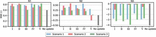
The results are mixed. When aggregating all results across all events, methods and scenarios of assimilating water-level data in one location at a time, it can be said that the assimilation leads to a significant improvement in the accuracy of water-level simulations in the outlet (N1), compared to model runs for the same location without rainfall updates.

The NSE values for initial model runs for N2 are quite low and, after correction, the NSE rose to reasonably high values. One can observe a difference in the effectiveness of the correction methods at N2: methods II and IV have led to better results among the five methods tested. Nevertheless, we can also observe that, in general, all the methods improved the model accuracy, especially considering that the average NSE without the updates is about – 0.56. Only Method III did not perform well when assimilating data at the other monitoring locations (N1 and N3), concerning the accuracy of model runs at location N2.

Input model updating through all methods and scenarios of DA improved the NSE of the water-level simulations at N3, but the results are still not satisfactory. For this location, it is evident that methods II and IV performed better. Also, all the methods led to better simulation results for N3 when assimilating data on-site (Scenario 2). It is important to note that the area upstream of this location is the smallest among the three analysed here. In addition, this region has the lowest percentage of impermeable area (Table 3). These two factors combine to reduce the effects of increasing or decreasing rainfall input values for that location compared to the other two monitoring locations, which have a larger associated runoff coefficient with the catchment areas upstream from them.

It can be seen that when assimilating data from one sensor at a time, the correction methods II and IV performed better than the others. Methods I, III and V showed good results, but in some situations when assimilating water-level data from one location, the effect on the simulations in the other locations was negative. Taking into account the advantage of methods II and IV, they are selected to further analyse the influence of their correcting effects on hydrographs.

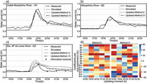
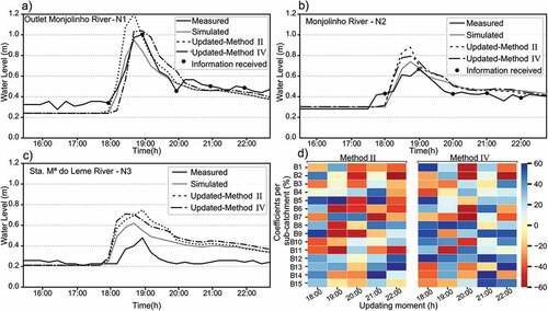
Figure 6 shows the hydrographs at the three monitoring locations N1, N2 and N3 when assimilating data at N3 by methods II and IV. Analysing the percentage of rainfall changes for each sub-catchment by the two methods (Fig. 6(d)), one may observe that both led mostly to rainfall input reduction (depicted by red), instead of rainfall input increase (blue). These results are consistent with the fact that the simulated hydrograph is overestimated. The hydrograph at N3 (Fig. 6(c)) shows that the updates made at 19:00 and 20:00 h are the most important for correcting rainfall inputs at this event because, at these moments, the simulated water level has significant errors. On the one hand, the correction at 19:00 h by Method II led to rainfall input increase at sub-catchment B1 and decrease at sub-catchment B5. After the update, the simulation results improved immensely, reducing simulated water levels to values very close to those observed. On the other hand, in the assimilation at 20:00 h, the updates for catchments B1 and B5 reduced approximately 60% the rainfall input values and, despite this significant amount of rainfall reduction, it is not enough for the model to reach the observed water levels.

Figure 6. The three hydrographs show the water levels observed, simulated and resulting from updates by the methods II and IV during event 2 at: a) location N1; b) location N2; c) location N3; and d) shows the percentage of rainfall changes for each sub-catchment. The updates are performed by assimilating water-level data from sensor N3 (scenario 2), every hour during the rainfall event.

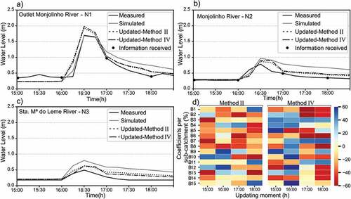
Figure 7(c) shows the results for assimilating data at N3 (Scenario 2) during rainfall event 4. Neither of the two correcting methods has led to a satisfactory increase in NSE for location N3. Method II resulted in an increased NSE from – 6.77 to 0.06 and Method IV in an increase to – 0.44. After 14:00 h, the model overestimated the water levels. For Method II, we can see that for the critical period between 14:00 and 18:00 h, the optimum correcting coefficients obtained for sub-catchments B1 and B5 led to a reduction in rainfall input but, still, the model underestimated water levels. For Method IV, a similar situation may be observed.

Figure 7. The three hydrographs show the water levels observed, simulated and resulting from updates by the methods II and IV during event 4 at: a) location N1; b) location N2; c) location N3; and d) shows the percentage of rainfall changes for each sub-catchment. The updates are performed by assimilating water-level data only from sensor N3 (scenario 2), every hour during the rainfall event.

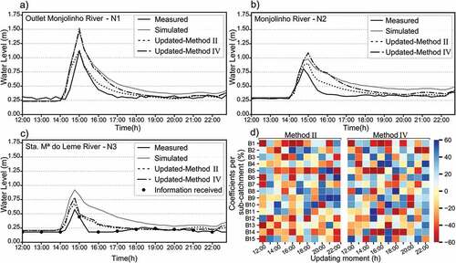
The simulated hydrographs for locations N1 and N2, in Fig. 7(a) and (b), respectively, are overestimated and, after optimization of the coefficients to correct rainfall based on water-level data assimilated at N3, the error for these two points was reduced by both correction methods. Method II achieved better results for N1 and N2, increasing the NSE from – 0.10 to 0.75 and from – 1.78 to 0.43, respectively. Method IV also led to an improvement in the results, but by less than Method II, with the NSE at N1 increasing from – 0.1 to 0.25 and at N2 from – 1.78 to – 1.26. In general, the optimal coefficients have reduced the rainfall inputs in both methods. It is important to emphasize that the approach of Method II does not reduce rainfall inputs just backwards, but also changes the rainfall values forward from the moment of data assimilation. Consequently, updates in the simulation can be more significant when using Method II.

5.3 Assessing model accuracy when assimilating data from multiple sensors

From the results presented in Section 5.2, assimilating data from one sensor at a time, methods II and IV performed better than the other updating methods. Taking this into account, scenarios for assimilating water-level data from multiple sensors at the same time are tested only for these two rainfall update methods (II and IV).

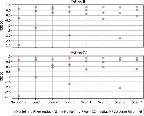
Figure 8 shows the overall NSE results for scenarios 4–7 at the three monitoring locations (N1–N3). For the two correction methods and all scenarios, the data assimilation resulted in improved NSE values. For locations N1 and N2, the accuracy of the model when assimilating data by Method IV is slightly better than that by Method II.

Figure 8. NSE results of all the rainfall events in the three monitoring locations N1, N2 and N3, when assimilating water-level data from multiple sensors at the same time (scenarios 4, 5, 6 and 7) by methods II and IV.

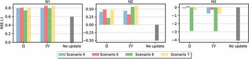
For location N1, all the results are very good. Scenario 7, when assimilating data at N2 and N3 at the same time, gave higher NSE values for N1 than when assimilating data on-site in the same time as other monitoring locations (scenarios 4, 5 and 6). For N2, the NSE results are also good and the best results are achieved in Scenario 7. However, for location N3, the NSE is quite low. Through Method II, when assimilating water-level data at N1 and N3 (Scenario 5), the simulation results at N3 showed a slight improvement. The worst results for N3 were obtained when assimilating data in the other two monitoring locations N1 and N2 (Scenario 6). Even then, the NSE results for N3 improved when compared to the simulation accuracy without correcting rainfall.

Table 5 presents the detailed NSE results for all scenarios and each rainfall event by the two methods tested. Figure 9 shows interesting results for assimilating water-level data at N1 and N2 at the same time (Scenario 3). The event presented in the hydrographs happened almost entirely between 18:00 and 20:00 h. The hourly updates with observed data are not enough to satisfactorily update the rainfall that affects the rise and fall of the flood wave. Furthermore, DA at untimely moments makes the model overestimate the water levels for both methods II and IV. It can be seen in Fig. 9(a) that, when the first information is assimilated at 18:00 h, the model slightly underestimates the values compared to the observation; then, the optimization based on this data aimed to increase the rainfall inputs. When new information is received subsequently at 19:00, the peak time has already passed and the previous correction leads to an overestimation of the peak. DA at locations N1 and N2 led to even worse results for N3. Since the beginning of the event at N3 (Fig. 9(c)), the hydrograph was overestimated and the increase in rainfall input values by DA led to a further increase in water levels.

Table 5. Performance results (NSE) for each rainfall event comparing the water levels measured at the monitoring locations with the model simulations for scenarios tested by methods II and IV in the second rainfall updating experiment.

No update	N1	N2	N3	N1	N2	N3	N1	N2	N3	N1	N2	N3
	Event 1			Event 2			Event 3			Event 4
	0.89	0.77	0.69	0.79	0.69	–4.46	0.80	–1.71	–5.80	–0.10	–1.78	–6.77
Method II
Scenario 4	0.96	0.85	0.94	0.83	0.75	–1.08	0.86	–0.56	0.24	0.52	0.59	–0.62
Scenario 5	0.93	0.86	0.94	0.75	–4.38	–0.54	0.87	0.02	–0.30	0.68	0.49	0.45
Scenario 6	0.95	0.68	0.76	0.62	0.32	–8.95	0.85	0.48	–0.98	0.54	–0.62	–2.43
Scenario 7	0.92	0.91	0.92	0.59	0.48	–1.33	0.91	0.14	–0.45	0.77	0.36	–0.41
Method IV
Scenario 4	0.94	0.79	0.84	0.78	0.59	–2.09	0.87	–0.19	–1.44	0.61	0.58	–0.30
Scenario 5	0.94	0.75	0.80	0.85	0.46	–1.25	0.86	–0.39	–0.33	0.73	0.49	–0.37
Scenario 6	0.95	0.81	0.79	0.72	0.48	–9.96	0.85	0.21	–0.26	0.64	0.77	–2.30
Scenario 7	0.93	0.82	0.86	0.79	0.67	–1.28	0.91	0.36	–2.64	0.77	0.58	–0.10

Figure 9. The three hydrographs show the water levels observed, simulated and resulting from updates by the methods II and IV during event 4 at: a) location N1; b) location N2; c) location N3; and d) shows the percentage of rainfall changes for each sub-catchment. The updates are performed by assimilating data from sensor N1 and N2 at the same time (scenario 6), every hour during the rainfall event.

For Event 3, when assimilating water-level data from sensor N1 and N2 (Fig. 10(a) and (b)), the results for both methods are very similar. For location N1, the rainfall input correction caused the peak to be slightly overestimated, while the original simulation was accurate. The falling limb of the model overestimated values and the updates in rainfall made the water-level decay faster, reaching values nearer to those observed in the hydrograph. Methods II and IV resulted in increases in NSE for this event at N1 from 0.8 to 0.85. At location N2, the simulated water levels are slightly ahead of the observed ones. The rainfall updates help to reduce the water-level values that are overestimated, but it is not able to correct the advance of the hydrograph concerning the observed one. For N3, the simulation errors were reduced by the updates as well (Fig. 10(c)). At this location, the simulated hydrograph was also overestimated compared to the observed one. The reduction of rainfall inputs helped to adjust the water-level values also at this location.

Figure 10. The three hydrographs show the water levels observed, simulated and resulting from updates by the methods II and IV during event 3 at: a) location N1; b) location N2; c) location N3; and d) shows the percentage of rainfall changes for each sub-catchment. The updates are performed by assimilating data from sensor N1 and N2 at the same time (Scenario 6), every hour during the rainfall event.

5.4 Summary of the effectiveness of the methods applied

Differences in rainfall events influence the effectiveness of data assimilation methods. After evaluating all the methods and scenarios, one at a time, a comparison of effectiveness is made for methods II and IV considering all the data series and scenarios together. In order to compare them, we averaged the NSE of all rainfall events and for each scenario of receiving sensor data at different locations. The efficiency measures are calculated separately for each monitoring location. Figure 11 shows the result of this comparison.

Figure 11. Comparison between DA methods II and IV by the mean NSE of all rainfall events used in this study. The values show the results obtained for all the proposed data assimilation scenarios (scen.).

Analysing the results for location N1, we can observe that the effectiveness of both methods is similar. Although the average NSE for all events is already at a satisfactory value without correcting, both approaches were able to improve the estimates slightly. At location N2, the correction methods had similar effectiveness but with some discrepancies. For scenarios 2 and 3, Method II shows better results and for scenarios 5 and 6, Method IV is more effective. Therefore, from these results at N2, it is not possible to define a clear difference in effectiveness between the two methods. Among the three monitoring locations, N3 is where the model presents the most significant errors in producing the estimates. Method II changes the rainfall values in the previous moments when the information is received and also after that. Because of this, the correction is slightly higher than by Method IV (which changes values of rainfall just going back from the moment when information is received). As a result, for location N3, it is possible to identify slightly better effectiveness of Method II.

It is interesting to note that in Scenario 4 (Fig. 11), when assimilating data from the three sensors, the model accuracy gained by both methods is higher but very marginal compared to the other scenarios assimilating data from two or only one sensor. The low performance gained when the number of sensors is increased might be explained by the nested nature of the sub-catchments where the sensors are installed. Since their flow must be correlated, any correction made in one location by the data assimilation will also be propagated in the others. Sensors N1 and N2 are located on the Monjolinho River in a cemented part of the canal, while sensor N3 is located in a tributary of the Monjolinho River that has natural coverage of the canal bed and a smaller cross-section compared to the ones of sensors N1 and N2. Taking these considerations into account, it is expected that water levels registered by sensors N1 and N2 will have more correlated behaviour compared to sensor N3. Looking at the results for scenarios 1, 3 and 6, which have in common the fact that they do not assimilate data from sensor N3, it can be seen that they show a less significant improvement in the effectiveness of the simulations for location N3. This has probably happened because they are receiving data only from sensors N1 and N2 that are not as correlated to sensor N3 data.

Another aspect that needs to be assessed is the coefficient values for rainfall correction. According to the results demonstrated by the sensitivity analysis of the model to the rainfall variation, some sub-catchments are much more responsive to rainfall. It is quite logical to assume that the optimization method has given more emphasis to rainfall variation at these catchments. However, it should be noted that the values found are quasi-optimal because of the mentioned time constraint assigned to the search algorithm: the DA method is developed to run for real-time operation in basins with rapid responses to rainfall, so optimization cannot run for longer that the predetermined (short) time step.

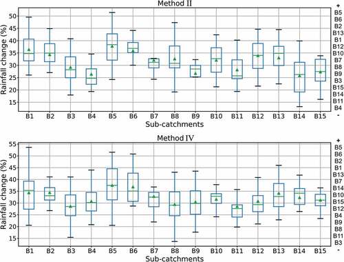
Figure 12 shows boxplots of the average percentage of rainfall variation at all scenarios analysed in each sub-catchment by correction methods II and IV. According to the sensitivity analysis of the model to rainfall inputs variation, the six most sensitive sub-catchments in descending order are B12, B6, B8, B13, B2 and B10, while the other catchments are almost non-sensitive. The six sub-catchments with the most significant variation in rainfall given by the optimization for the updating Method II are B5, B6, B2, B13, B1 and B12. Sub-catchments B5 and B1 have low sensitivity to rainfall according to the sensitivity analysis and, contrary to the expected, their rainfall inputs are changed considerably, as determined by optimization, while the very sensitive sub-catchments B8 and B10 are not the ones with the largest coefficients of rainfall change. By Method IV, sub-catchments B6, B2 and B13 have high percentage values of rainfall changes compared to the others. However, the non-sensitive sub-catchment B1 is the one with the highest rainfall DA update.

Figure 12. Box plots of the average of rainfall variation of the seven scenarios of model input correction by method II and IV. Values calculated for sub-catchments B1 to B15.

6 Summary and conclusions

This research proposed a data assimilation method to update rainfall inputs of an urban semi-distributed hydrological model as response of real-time water-level observations. The method was validated on the Monjolinho catchment and five different experiments were performed. The assimilation performance was evaluated by assessing the improvement in model accuracy when data were from different locations and when the number of sensors providing water-level observations was increased.

This study has shown that model outputs are sensitive to rainfall variation, in particular when the original input values are increased. This demonstrantes that a deterministic method of input correction have the potential to improve water-level simulations. Assimilation of water-level data from only one sensor, for all the methods and regardless of its location in the catchment, led to an improvement in the water-level simulations (albeit not significantly). Moreover, the NSE values improved as the number of sensors was increased. However, the improvement in simulation accuracy when increasing the number of sensors was not particularly notable. Thus, it is fundamental to properly assess the trade-off between the cost of installing several sensors and the gain in model accuracy.

The main limitation of this study was the deterministic approach of the updating procedure, which does not consider the uncertainties of the model and the observed data. Moreover, this study only used deterministic rainfall from raingauges, whereas numerical weather predictions and remote sensing products are increasingly used and recommended for flood forecasting models. Besides, the model was only tested as a case study on the Monjolinho catchment and further comparison in other catchments, for various rainfall–runoff events and several combinations and quantities of physical sensors may ultimately contribute to help us understand the accuracy gained due to the number of water-level sensors.

For future studies, we suggest that the possibility of using faster models than SWMM (or its surrogates) and other optimization schemes be explored. Here, we assimilated data from traditional water-level sensors at a regular interval of one hour. It is recommended that the effect of increasing or decreasing the assimilation interval on model accuracy could be assessed – this should allow us to evaluate the usefulness of the method when using other sources of data, such as (asynchronous) data from citizen observatories, which also has varying uncertainty.

The proposed assimilation method for updating uncertain rainfall inputs of urban hydrodynamic models is a simple way to circumvent the limitation of nonlinear correlation between observation and model states. It has the potential to improve flood forecasting simulation for locations that require rapid responses, where, for example, ensemble-based assimilation methods would be infeasible, in terms of computational effort. The presented approach is a promising tool for increasing the accuracy of urban hydrodynamic modelling and forecasting and, hence, contributing to making cities more resilient to floods.

Declaration of originality

The author(s) hereby declare previous originality check, no conflict of interest and open access to the repository of data used in this paper for scientific purposes.

Acknowledgements

The authors would like to thank the research funding grants provided by: project CAPES Pró Alertas CEPED/USP [grant No 88887.091743/2014-01], project INCT-II (Climate Change, Water Security) funded by the National Council for Scientific and Technological Development (CNPq) [grant No 465501/2014-1] and São Paulo Research Foundation (FAPESP) [grant No 2014/50848-9], project CNPq (EESC-USPCEMADEN/MCTIC) [grant No 312056/2016-8], CAPES School of Advanced Studies of Water and Society under Change [grant No 88881.198361/2018-01] and CAPES PROEX (PPG-SHS, EESC-USP).

Disclosure statement

No potential conflict of interest was reported by the authors.

Data and software availability

The data assimilation software for methods I–V and the SWMM calibrator tool are developed in Python 3.6. All the data used in this paper and the SWMM calibrator tool are available for download at the GitHub platform https://github.com/mclarafava/Data-Assimilation; https://github.com/mclarafava/SWMM-calibrator.

Additional information

Funding

This study was financed in part by the Coordenação de Aperfeiçoamento de Pessoal de Nível Superior - Brasil (CAPES) - Finance Code 001, the Graduate Program in Hydraulic Engineering and Sanitation (CAPES PROEX, PPG-SHS), the project CAPES Pró Alertas CEPED/USP [grant No 88887.091743/2014-01], the project INCT-II (Climate Change, Water Security) funded by the National Council for Scientific and Technological Development (CNPq) [grant No 465501/2014-1] and São Paulo Research Foundation (FAPESP) [grant No 2014/50848-9], and the project CNPq (EESC-USP CEMADEN/MCTIC) [grant No 312056/2016-8].

References

- Andrieu, C., Doucet, A., and Holenstein, R., 2010. Particle Markov chain Monte Carlo methods. Journal of the Royal Statistical Society: Series B (Statistical Methodology), 72 (3), 269–342.
- Ashley, R.M., et al.,2005. Flooding in the future–predicting climate change, risks and responses in urban areas. Water Science and Technology, 52 (5), 265–273.
- Bai, T., et al.,2018. The hydrologic role of urban green space in mitigating flooding (Luohe, China). Sustainability, 10 (10), 3584.
- Barros, R.M., Mendiondo, E.M., and Wendland, E., 2007. Cálculo de áreas inundáveis devido a enchentes para o plano diretor de drenagem urbana de São Carlos (PDDUSC) na bacia escola do córrego do Gregório. Revista Brasileira De Recursos Hídricos, 12, 5–17.
- Borup, M., et al., 2018. Technical note on the dynamic changes in Kalman gain when updating hydrodynamic urban drainage models. Geosciences, 8 (11), 416.
- Chen, H., et al., 2013. Hydrological data assimilation with the Ensemble Square-Root-Filter: use of streamflow observations to update model states for real-time flash flood forecasting. Advances in Water Resources, 59, 209–220.
- Collier, C.G., 2007. Flash flood forecasting: what are the limits of predictability?. Quarterly Journal of the Royal Meteorological Society, 133 (622), 3–23.
- Coustau, M., et al., 2013. Benefits and limitations of data assimilation for discharge forecasting using an event-based rainfall-runoff model. Natural Hazards and Earth System Science, 13, 583–596.
- Cronshey, R., 1986. Urban hydrology for small watersheds. Washington, DC: US Dept. of Agriculture, Soil Conservation Service, Engineering Division.
- Divac, D., et al.,2009. A procedure for state updating of SWAT-based distributed hydrological model for operational runoff forecasting. Journal of the Serbian Society for Computational Mechanics, 3 (1), 298–326.
- Evensen, G., 2003. The ensemble Kalman filter: theoretical formulation and practical implementation. Ocean Dynamics, 53 (4), 343–367.
- Fortin, F.A., et al., 2012. DEAP: evolutionary algorithms made easy. Journal of Machine Learning Research, 13, 2171–2175.
- Francois, C., Quesney, A., and Ottlé, C., 2003. Sequential assimilation of ERS-1 SAR data into a coupled land surface–hydrological model using an extended Kalman filter. Journal of Hydrometeorology, 4 (2), 473–487.
- Hansen, L.S., et al.,2014. Flow forecasting using deterministic updating of water levels in distributed hydrodynamic urban drainage models. Water, 6 (8), 2195–2211.
- Harader, E., et al.,2012. Correcting the radar rainfall forcing of a hydrological model with data assimilation: application to flood forecasting in the Lez catchment in southern France. Hydrology and Earth System Sciences, 16 (11), 4247–4264.
- He, X., et al., 2017. Using data assimilation in real-time hydrological modeling of groundwater and stream flow in Silkeborg, Denmark. In: AGU Fall Meeting Abstracts, New Orleans, LA.
- Hutton, C.J., et al.,2012. Dealing with uncertainty in water distribution system models: A framework for real-time modeling and data assimilation. Journal of Water Resources Planning and Management, 140 (2), 169–183.
- Hutton, C.J., et al., 2014. Real-time data assimilation in urban rainfall-runoff models. Procedia Engineering, 70, 843–852.
- Instituto Brasileiro de Geografia e Estatística (IBGE) (Brazilian Institute of Geography and Statistics), 2018. Estimativas da população residente no Brasil e unidades da federação com data de referência em 1º de julho de 2018 (Estimates of the resident population in Brazil and in units of the federation with reference date July 1, 2018). Available from: https://www.ibge.gov.br/estatisticas/sociais/populacao/9103-estimativas-de-populacao.html?=&t=o-que-e [Accessed 5 February 2019].
- Kahl, B. and Nachtnebel, H.P., 2008. Online updating procedures for a real-time hydrological forecasting system. IOP Conference Series: Earth and Environmental Science, 4 (1), 012001. IOP Publishing.
- Lindström, G., 2016. Lake water levels for calibration of the S-HYPE model. Hydrology Research, 47 (4), 672–682.
- Liu, Y., et al.,2012. Advancing data assimilation in operational hydrologic forecasting: progresses, challenges, and emerging opportunities. Hydrology and Earth System Sciences, 16 (10), 3863–3863.
- Liu, Y. and Gupta, H.V., 2007. Uncertainty in hydrologic modeling: toward an integrated data assimilation framework. Water Resources Research, 43 (7), W07401.
- Maybeck, P.S., 1982. Stochastic models, estimation, and control (Vol. 3). New York, NY: Academic Press.
- Mazzoleni, M., et al.,2018a. Data assimilation in hydrologic routing: impact of model error and sensor placement on flood forecasting. Journal of Hydrologic Engineering, 23 (6), 04018018.
- Mazzoleni, M., et al.,2018b. Real-time assimilation of streamflow observations into a hydrological routing model: effects of model structures and updating methods. Hydrological Sciences Journal, 63 (3), 386–407.
- McMillan, H., et al.,2011. Rainfall uncertainty in hydrological modelling: an evaluation of multiplicative error models. Journal of Hydrology, 400 (1–2), 83–94.
- McMillan, H.K., et al.,2013. Operational hydrological data assimilation with the recursive ensemble Kalman filter. Hydrology and Earth System Sciences, 17 (1), 21–38.
- Mendes, H.C. and Mendiondo, E.M., 2007. Histórico da expansão urbana e incidência de inundações: O Caso da Bacia do Gregório, São Carlos–SP. Revista Brasileira De Recursos Hídricos, 12 (1), 17–27.
- Moradkhani, H., et al.,2005. Uncertainty assessment of hydrologic model states and parameters: sequential data assimilation using the particle filter. Water Resources Research, 41 (5), W05012.
- Moradkhani, H., DeChant, C.M., and Sorooshian, S., 2012. Evolution of ensemble data assimilation for uncertainty quantification using the particle filter‐Markov chain Monte Carlo method. Water Resources Research, 48 (12), W12520.
- Nash, J.E. and Sutcliffe, J.V., 1970. River flow forecasting through conceptual models part I—A discussion of principles. Journal of Hydrology, 10 (3), 282–290.
- Pathirana, A., 2015. SWMM5 calls from python (version 1.1.0.2) [Computer software]. Python Package Index (PyPI) repository. Available from https://pypi.org/project/SWMM5/ [Accessed 5 June 2018].
- Pedersen, J.W., et al., 2016. Evaluation of maximum a posteriori estimation as data assimilation method for forecasting infiltration-inflow affected urban runoff with radar rainfall input. Water, 8 (9), 381.
- Refsgaard, J.C., 1997. Validation and intercomparison of different updating procedures for real-time forecasting. Hydrology Research, 28 (2), 65–84.
- Reichle, R.H., McLaughlin, D.B., and Entekhabi, D., 2002. Hydrologic data assimilation with the ensemble Kalman filter. Monthly Weather Review, 130 (1), 103–114.
- Romero, G.B., 2016. Dinâmica ecohidrológica de rios urbanos no contexto de gestão de riscos de desastres. Thesis (MSc). University of São Paulo.
- Rossman, L.A., 2010. Storm water management model user’s manual, version 5.0. Cincinnati: National Risk Management Research Laboratory, Office of Research and Development, US Environmental Protection Agency.
- Rossman, L.A. and Huber, W., 2016. Storm water management model reference manual volume I–hydrology (Revised). Cincinnati, OH, USA: US Environmental Protection Agency.
- Segond, M.L., Wheater, H.S., and Onof, C., 2007. The significance of spatial rainfall representation for flood runoff estimation: A numerical evaluation based on the Lee catchment, UK. Journal of Hydrology, 347 (1–2), 116–131.
- Seo, D.J., et al.,2009. Automatic state updating for operational streamflow forecasting via variational data assimilation. Journal of Hydrology, 367 (3–4), 255–275.
- Seo, D.J., Koren, V., and Cajina, N., 2003. Real-time variational assimilation of hydrologic and hydrometeorological data into operational hydrologic forecasting. Journal of Hydrometeorology, 4 (3), 627–641.
- Stanzel, P., et al., 2008. Continuous hydrological modelling in the context of real time flood forecasting in alpine Danube tributary catchments. IOP Conference Series: Earth and Environmental Science, 4 (1), 012005. IOP Publishing.
- Thiboult, A. and Anctil, F., 2015. On the difficulty to optimally implement the Ensemble Kalman filter: an experiment based on many hydrological models and catchments. Journal of Hydrology, 529, 1147–1160.
- Tollan, A., 2002. Land-use change and floods: what do we need most, research or management? Water Science and Technology, 45 (8), 183–190.
- Walker, J.P. and Houser, P.R., 2005. Hydrologic data assimilation. Advances in Water Science Methodologies, 1, 25–48.
- World Meteorological Organization (WMO), 2011. Manual on flood forecasting and warning. WMO, No. 1072.
- Xie, X. and Zhang, D., 2010. Data assimilation for distributed hydrological catchment modeling via ensemble Kalman filter. Advances in Water Resources, 33 (6), 678–690.
- Yang, G., et al.,2011. The impact of urban development on hydrologic regime from catchment to basin scales. Landscape and Urban Planning, 103 (2), 237–247.
- Yin, J., et al., 2016. Evaluating the impact and risk of pluvial flash flood on intra-urban road network: A case study in the city center of Shanghai, China. Journal of Hydrology, 537, 138–145.
- Young, P.C., 2002. Advances in real–time flood forecasting. Philosophical Transactions of the Royal Society of London A: Mathematical, Physical and Engineering Sciences, 360 (1796), 1433–1450.
- Zawadzki, I.I., 1973. Statistical properties of precipitation patterns. Journal of Applied Meteorology, 12 (3), 459–472.