Assessing parameter identifiability for multiple performance criteria to constrain model parameters

ABSTRACT

Reliable simulations of hydrological models require that model parameters are precisely identified. In constraining model parameters to small ranges, high parameter identifiability is achieved. In this study, it is investigated how precisely model parameters can be constrained in relation to a set of contrasting performance criteria. For this, model simulations with identical parameter samplings are carried out with a hydrological model (SWAT) applied to three contrasting catchments in Germany (lowland, mid-range mountains, alpine regions). Ten performance criteria including statistical metrics and signature measures are calculated for each model simulation. Based on the parameter identifiability that is computed separately for each performance criterion, model parameters are constrained to smaller ranges individually for each catchment. An iterative repetition of model simulations with successively constrained parameter ranges leads to more precise parameter identifiability and improves model performance. Based on these results, a more consistent handling of model parameters is achieved for model calibration.

KEYWORDS:

• Parameter identifiability
• multiple performance criteria
• diagnostic model analysis
• parameter constraints
• parameter space reduction

Editor A. Fiori Associate editor A. Efstratiadis

1 Introduction

Reliable model simulations requires, among others, the selection of an appropriate model structure, suitable input data as well as precise identification of model parameter values which is in the focus of this study. Hydrological models include parameters for adaptation to the specific hydrological conditions of the study catchments. Each parameter influences one or more hydrological processes. For hydrologically consistent modelling, parameter values need to be identified precisely so that they represent the associated processes accurately (Wagener et al. 2003, Shin et al. 2015). A strong relationship between model parameter and corresponding hydrological process facilitates the identification of parameter values (Guse et al. 2017). To identify appropriate model parameter values, typically, a large number of model simulations with different parameter combinations is carried out and analysed according to their impact on performance criteria. Performance criteria is here used as a joint term for statistical performance measures, e.g. NSE, KGE (Nash and Sutcliffe 1970, Gupta et al. 2009) and signature measures (see Section 3.2 for definitions).

In this context, parameter identifiability assesses how precisely the values for a model parameter can be identified (Wagener et al. 2003). Hereby, it is aimed to constrain model parameters to reasonable ranges. The more the model parameter ranges are reduced, the more precisely a parameter is identified. High identifiability means that model performance is optimal within this parameter range. In the best case, the values of model parameters are in a small range within all behavioural combinations of model parameters (Wagener et al. 2003, Abebe et al. 2010). In this case, a model parameter can be strongly constrained to these values. A smaller range also reduces the impact of equifinality and thus reduces the uncertainty in selecting adequate parameter values (Wagener et al. 2001, Kelleher et al. 2013, Shin et al. 2015). A narrow range within the behavioural parameter sets (high parameter identifiability) provides a clear estimation of the parameter value and confidence that the processes are accurately simulated by the model (Wagener and Kollat 2007, Abebe et al. 2010, Cibin et al. 2010). In contrast, in the case model performance is similar for all parameter values, parameter identifiability is low and the best values for these parameters are unclear.

Parameter identifiability varies depending on the selected performance criteria (Wagener et al. 2001, 2003). Ideally, each criterion has a different focus and thus captures different hydrological conditions (Gupta et al. 1998, Boyle et al. 2000, Reusser et al. 2009). It is common practice to integrate several performance criteria focusing on the evaluation of different catchment processes (Arnold et al., 2015, Yilmaz et al. 2008, Pokhrel et al. 2012, Yen et al. 2014, Pfannerstill et al. 2017). However, the use of contrasting performance criteria that are focused on different hydrological aspects leads to a trade-off between them in optimising parameter values, since the selected best parameter values are likely to be different between these criteria (Kiesel et al. 2017). For instance, a parameter value which leads to a good representation of high flows can fail in reproducing low flows and vice versa (Madsen 2000, Boyle et al. 2001, Bekele and Nicklow 2007, Kumar et al. 2010, Zhang et al. 2011, Pfannerstill et al. 2014b).

While parameter identifiability may be precisely estimated by one performance criterion, it could be low for another criterion (Wagener et al. 2001, Fenicia et al. 2008). With each additional and contrasting performance criterion, the parameter ranges are further reduced and reasonably constrained (Yilmaz et al. 2008, Pechlivanidis et al. 2014, Westerberg et al. 2014), but may also cause contradictive results.

Three cases of parameter identifiability can be distinguished: (1) precise identification is achieved by deriving the same best parameter values using different performance criteria; (2) parameter identifiability is low in the case of low relationship between parameter variations and values of all performance criteria; and (3) the best parameter values are contradictive between different performance criteria.

In addition, parameter identifiability can be different between contrasting catchments which are characterized by differences in catchment characteristics and the dominance of processes and model parameters (Guse et al. 2019). Hence, the most precise estimations are usually obtained for the most dominant processes (Kelleher et al. 2013). Moreover, the issue of identifiability becomes more complicated for higher model complexity and increasing number of parameters (Martinez and Gupta 2011).

By constraining a model parameter, also the overall parameter space is reduced (Hogue et al. 2006). This leads to a denser parameter sampling since the distance between two parameter sets is reduced in the x-dimensional parameter space. Thus, a better coverage of parameter space is achieved by reducing the ranges of model parameters. Due to that, the probability to detect a good parameter combination is increased. Moreover, physically unrealistic parameter combinations are avoided to finally represent the relevant hydrological characteristics of the catchment more realistically (Arnold et al., 2015). Due to precise parameter identification and a smaller parameter space, it is expected that better parameter space coverage also improves model performance (Gharari et al. 2014, Zink et al. 2018).

The aim of this study is to constrain model parameters consistently and objectively to reasonable ranges to achieve a better process representation in the model and thus increasing its model performance. To achieve this aim, the following research questions are stated:

1. How does the identifiability of model parameters vary between contrasting performance criteria?

2. Can a model parameter consistently be constrained or does parameter identifiability lead to contrasting suitable parameter ranges?

3. How does a refinement of the parameter space impact parameter identifiability and model performance?

To answer these questions, identifiability of model parameters is computed based on multiple performance criteria to constrain parameter ranges. To investigate spatial variability in parameter identification, this procedure is applied in three contrasting catchments. Model simulations and computation of parameter identifiability are repeated for a refined parameter space. It is further analysed how overall model performance is impacted by the refinement of parameter space.

2 Study catchments

To test our methodology under varying conditions, three catchments were selected that are contrasting in terms of catchment characteristics and dominant processes as shown in Guse et al. (2019). The catchments vary in elevation from lowlands via mid-range mountains to alpine (in increasing order of elevation). The Treene has a catchment size of 481 km² and is located in the lowlands of northern Germany. The catchment is strongly dominated by a single process, i.e. groundwater flow (Pfannerstill et al. 2015, Guse et al. 2016), whereas the impacts of snow and surface runoff are low. In summer, evapotranspiration is also a dominant process. The Kinzig is a 925-km²-sized subcatchment of the Rhine basin and is located in the mid-range mountains. It has an elevation gradient of 98–628 m a.s.l. and the main land cover is forest and pasture. The Kinzig catchment is subject to a complex interaction of snowmelt, surface runoff, interflow and groundwater flow. The Ammer is a 602 -km²-sized subcatchment of the Danube basin and is located in the southern German Alpine region. It has an elevation gradient of 547–2157 m a.s.l. and, similar to the Kinzig, is mainly covered by forest and pasture. The hydrology of the Ammer catchment is mainly governed by snow and surface processes (for more details, see Guse et al. 2019).

3 Methods

3.1 Soil and Water Assessment Tool (SWAT)

For hydrological modelling, the Soil and Water Assessment Tool (SWAT; Arnold et al. 1998) was selected in its modified version, SWAT3s, which includes two active aquifers (Pfannerstill et al. 2014a). In naming SWAT in this study, we always refer to the SWAT3s model version. The SWAT model computes all major hydrological processes at a daily resolution and provides daily outputs of discharge and other hydrological processes. Its spatial discretization is based on subbasins and hydrological response units (HRU) with same catchment information in terms of land use, soil and slope classes. For the model set-up in the three catchments we refer to Guse et al. (2016) for Treene, to Kakouei et al. (2018) for Kinzig, and to Kiesel et al. (2019) for Ammer. The SWAT model structure was diagnostically investigated and if required improved in previous studies (Guse et al. 2014, Pfannerstill et al. 2014a, 2015). Moreover, Guse et al. (2019) employed detailed analyses of the spatial variability in processes and model parameters across different catchments. This study is focused on the identification of parameter values. Based on these former studies, twelve model parameters were included to capture all relevant processes that are briefly characterized in Table 1. The knowledge of the model parameters was used to restrict the parameter ranges to realistic values for the three study catchments (see Guse et al. 2016, 2019). Identical parameter ranges were applied for all catchments.

Table 1. Table of SWAT model parameters (modified from Guse et al. 2017). Lower and upper ranges are given as absolute range (r), additive (a) or multiplicative (m) values. For further information we refer to the theoretical documentation of the SWAT model (Neitsch et al. 2011).

Parameter	Abbreviation	Process	Range Type	Lower Range	Upper Range
Snow fall temperature	SFTMP	Snow	r	–2.5	2.5
Snow melt temperature	SMTMP	Snow	r	–2.5	2.5
Curve number	CN2	Surface runoff	a	–15	5
Surface runoff lag time	SURLAG	Surface runoff	r	0.8	4
Lateral flow lag time	LATTIME	Lateral flow	r	0.2	8
Tile flow lag time	GDRAIN	Tile flow	m	0.5	1.5
Available water capacity of a soil layer	SOL_AWC	Soil water	a	–0.02	0.1
Saturated hydraulic conductivity of a soil layer	SOL_K	Soil water	m	0.5	3
Soil evaporation compensation factor	ESCO	Evapotranspiration	r	0.2	1
Groundwater delay time (fast aquifer)	GW_DELAYfsh	Groundwater	r	1	50
Aquifer fraction coefficient (slow aquifer)	RCHRGssh	Groundwater	r	0.2	0.8
Baseflow alpha factor (slow aquifer)	ALPHA_BFssh	Groundwater	r	0.001	0.2

3.2 Model simulations and performance criteria

The methodical approach was designed to identify the model parameters in a hydrologically meaningful way. To achieve this, 2000 parameter sets were generated based on Latin Hypercube sampling (Van Griensven et al. 2006), as described in Pfannerstill et al. (2014b) using the r-package FME (Soetaert and Petzoldt 2010). In this step, parameter ranges and parameter sets were identical in the 2000 model runs for all three catchments (LHinitial). The SWAT model was run from 1997 to 2010, split into a calibration period (2000–2005) and a validation period (2006–2010). The first three years were used as the warm-up period. The calibration period includes wet, normal and dry years.

Next, 2000 model runs were carried out. To evaluate the model performance in the three catchments, 10 different criteria were computed for all runs. Five statistical performance criteria were employed, namely the Nash-Sutcliffe efficiency (NSE) (Nash and Sutcliffe 1970) and the Kling-Gupta efficiency (KGE) (Gupta et al. 2009, Kling et al. 2012), as well as, separately, the three components of KGE, i.e. KGE_alpha (variability), KGE_beta (bias) and KGE_r (correlation). As signature measures, the ratio of the root mean square error to the standard deviation (RSR; Moriasi et al. 2007), was calculated individually for five segments of the flow duration curve (FDC), i.e. very high (0–5% days of exceedence), high (5–20%), medium (20–70%), low (70–95%) and very low (95–100%), as proposed by Pfannerstill et al. (2014b). It was detected which performance criterion has a good performance in which model runs and how the performance varies between the 10 performance criteria. Both, the generated parameter sets and the calculated performance criteria from these 2000 simulations were then used for the following analyses.

The suitability of this set of 10 performance criteria was demonstrated in Guse et al. (2017). It was shown that they are suitable to represent all phases of the hydrograph. In addition, the relationship between model parameters and performance criteria was analysed to show how strongly SWAT model parameters are connected to performance criteria in the Treene catchment (Guse et al. 2017). It was demonstrated that RSR for (very) high flows is suitable to identify accurate values of the surface runoff parameter curve number (CN2). The soil parameters SOL_AWC and ESCO strongly impact KGE_beta and RSR for mid flows and are thus related to the overall water balance. As the controlling parameter for droughts ALPHA_BFssh is related to RSR for very low flows. Moreover, Guse et al. (2017) showed that the correlation patterns between model parameters and performance criteria change between two contrasting catchments. For example, while a linear relationship between NSE and KGE was found in the Treene lowland catchment, we do not see a linear relationship in a mid-range mountain catchment which also results in a lower correlation between NSE and KGE. Thus, a set of 10 contrasting performance criteria was selected to ensure that spatial variability is considered.

3.3 Parameter identifiability

In this step, it was investigated which parameter values lead to good model performance. In this way, the identifiability of all parameters in relation to the 10 performance criteria was derived. Parameter identifiability can be evaluated by constructing parameter identifiability plots. For this, the probability density function (pdf) of model parameters was computed within their range. We estimated kernel density with the R-package stats (function density), showing the density of parameter values. For the initial parameter sampling and under consideration of all model runs, a straight line was detected which means that parameter values are evenly distributed and the parameter space is equally covered.

However, when selecting only the best model runs according to a certain performance criterion, the distribution of parameter values changes for relevant model parameters. Considering this, parameter identifiability plots are constructed for a subset of model simulations (Pechlivanidis et al. 2014). These plots show how the optimal parameter values are distributed for each performance criterion. The narrower the range of the parameter space and the higher the density, the higher is the parameter identifiability. In this way, the construction of identifiability plots allows to constrain model parameters by reducing the parameter ranges to values with high identifiability. In contrast, a (close to) straight line means that it is impossible to locate good model results. In this case, a model parameter is denoted as unidentifiable (Wagener et al. 2001, 2003). Thus, parameter identifiability plots show how precisely parameter values are identified for a specific performance criterion.

3.3.1 Parameter identifiability plots for initial parameter sets

Using 10 different performance criteria to construct parameter identifiability plots, it was aimed to identify parameter values precisely. For each criterion, the best parameter values were identified. A subset of the total number of model simulations was selected to calculate parameter identifiability. This subset included the best 500 model runs according to each criterion, i.e. which are among the 25% quantile, in the calibration period. A difference in parameter identifiability compared to the initial distributed parameter values indicates a reduction of the suitable parameter range according to the selected criterion.

Three options in terms of parameter identifiability can be distinguished:

1. High parameter identifiability means that the best model simulations according to one or more performance criteria lead to a reduction of the suitable parameter range and identifies parameter values in a narrower space.

2. Low parameter identifiability would be that none of the performance criteria leads to the precise parameter identification and it becomes unclear how to identify the parameter.

3. A contradictive result would be obtained in the case that the reduction of parameter range according to different performance criteria does not result in an overlay of the resulting suitable parameter range. In other words, one performance criterion suggests an increase to higher values, while others propose a reduction to lower values of a specific parameter.

3.3.2 Constrained parameter space

Parameter identifiability plots derived from the initial runs were used to reduce the range for each model parameter in each catchment based on the model performance in the calibration period. For constraining the parameter ranges, the maximum value of the density functions for all 10 performance criteria was computed for each parameter. Next, the parameter range was computed in which the parameter values reach at least half of the maximum value of the density function. This approach was repeated for each performance criterion. For the refinement of the parameter range, only the performance criteria that are related to this model parameter were used (Guse et al. 2017). For a given parameter, we only used criteria for which the maximum of the density functions was not more than 20% below the overall maximum value. The constrained range was set such that it covered the parameter ranges as refined by all selected performance criteria.

Three cases were possible:

1. Precisely identified parameters were constrained by reducing their ranges by x% of their initial ranges with 0 < x < 100%.

2. Unidentifiable parameters were not considered for the next parameter sampling round and the initial parameter values were used instead.

3. Contradictive identified parameters were still considered within their original ranges.

3.3.3 Parameter identifiability plots for constrained model parameters

Next, Latin Hypercube (LH) sampling with 2000 parameter sets and model simulations were repeated with constrained parameter space (LHconstrain). In this step, the selected model parameters and thus also the parameter sampling varied between the catchments due to differences in the identifiability of model parameters arising from catchment characteristics. Parameter identifiability plots were then constructed in a second round based on the refined parameter ranges. To evaluate the benefit of this refinement, the distribution of performance criteria was compared between the initial simulations and the simulations with constrained parameter ranges for the calibration period (2000–2005). This reduction of the parameter range and its re-sampling were repeated until no further reduction could be realized or no further improvement in the overall model performance could be achieved. At the end, the model performance was also computed separately for the independent validation period (2006–2010) for the initial parameter sampling and all rounds of parameter constraints, in order to evaluate the benefit of the presented approach.

3.3.4 Variability in modelled discharge between unconstrained and constrained parameters

Next, the benefit of constraining model parameter ranges was analysed in relation to the unconstrained case with initial parameter ranges. The 2000 model simulations of the initial and the final parameter ranges were compared. For both approaches, the 5% and the 95% uncertainty bounds of the discharge time series were computed for each day to compare whether the discharge variability among the model simulations has been changed and whether specific patterns are observed for certain hydrological conditions.

3.3.5 Coverage of parameter space

Subsequently, the benefit of reduced parameter ranges was analysed in terms of the coverage of the parameter space. Hereby, the impact of constrained parameter ranges was compared with an increase in the number of model simulations. The parameter sampling was repeated for LHinitial for 5000 model runs. Then, the Euclidean distance was calculated between all pairs of parameter sets for all approaches (LHinitial, LHinitial with 5000 runs, LHconstrain for the three catchments). To make the parameters comparable, their values were standardized in all approaches by a division with the standard deviation of the parameter values computed for LHinitial. The minimum Euclidean distance was next computed for each parameter set. Then, these 2000 (5000) minimum Euclidean distances were averaged for all parameter sets. The idea of this approach was that the minimum Euclidean distance shows the density of the parameter space sampling. The parameter space was better covered the smaller the Euclidean distance was.

4 Results

4.1 Parameter value identification

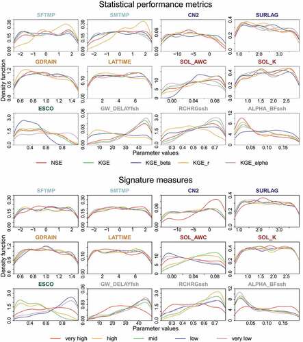
Figure 1 shows the parameter identifiability plots for statistical performance measures (above) and signature measures (below) for the Treene catchment as derived in LHinitial. Groundwater delay (GW_DELAYfsh) and aquifer partitioning coefficient (RCHRGssh) were precisely constrained by contrasting performance criteria such as RSR for low and high flows as well as by NSE, KGE and KGE_alpha. The most precise identifiability was found for the baseflow recession coefficient (ALPHA_BFssh) with the highest performance for low values as detected by RSR for very low flows. The curve number (CN2) was optimally identified by RSR for very high flow segment (slightly positive change in CN2). No improvement in the parameter value identification for all selected performance criteria was detected for three parameters related to fast runoff components (SURLAG, GDRAIN, LATTIME) and a soil parameter (SOL_K). A contradictive result was found for two soil parameters which regulate water balance, namely available soil water capacity (SOL_AWC) and the soil evaporation parameter ESCO. Both cases show a trade-off when simultaneously optimising low and high flows.

Figure 1. Parameter identifiability plot as density function for twelve SWAT model parameters for the Treene catchment computed for the calibration period (2000–2005). Different statistical metrics (above) and signature measures (below) are used to select behavioural parameter sets. The model parameter names are coloured according to the different hydrological processes.

The results of the parameter identifiability plots were then transformed into a coloured line and jointly shown for all catchments (Fig. 2). In the Kinzig catchment, precise identification was detected for snow parameters by NSE and KGE_r, for ESCO for several performance criteria as well as for ALPHA_BFssh for RSR for very low flows. In contrast, contradictive results were found for LATTIME, SOL_AWC, SOL_K and GW_DELAYfsh. In the Ammer catchment, parameter values were reduced for SFTMP by RSR for very high flows and increased for SMTMP by KGE, KGE_r and NSE. Both surface runoff parameters (CN, SURLAG) were constrained to low values by KGE, NSE, KGE_alpha and KGE_r. Lateral flow lag time (LATTIME) was constrained by several performance criteria. In the Ammer catchment, no trade-off was found between high, mid and low flows for all surface parameters. Contradictive results were found for two soil parameters SOL_AWC and SOL_K, while ESCO is constrained by KGE_beta. Among groundwater parameters, RCHRGssh was precisely identified by KGE_beta and RSR for mid and (very) low flows.

Figure 2. Presentation of appropriate parameter values for twelve model parameters in the three catchments using the initial parameter ranges. Appropriate parameter ranges are calculated for 10 different performance criteria. The colour gradient ranges from yellow (inappropriate parameter values) via green to blue (appropriate parameter values). The colour bar for each subplot is defined by setting the blue colour to the maximum value among all performance criteria. A greater colour contrast indicates a high parameter identifiability, while a low contrast indicates low identifiability. The model parameter names are coloured according to the different hydrological processes.

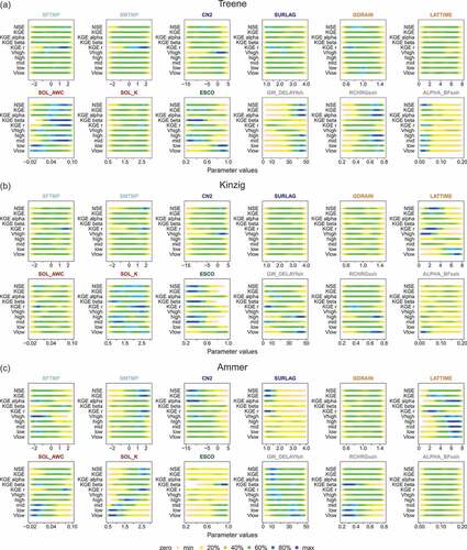
The comparison of parameter identifiability between the three catchments showed several similarities. In general, three types could be distinguished. Firstly, a precise range of the parameters was identified using one or more performance criteria. Baseflow recession (ALPHA_BFssh) was precisely identified by RSR for very low flows with the best performance for low values of ALPHA_BFssh. Thus, a strong water retention in the slow aquifer is required to maintain adequate low flow conditions under droughts in all catchments except of the Ammer catchment which only includes one (fast) aquifer.

Contradictive results between contrasting performance criteria were in particular found for water balance related parameters such as the soil evaporation (ESCO). Here, the identified best parameter ranges varied between RSR for low and mid flows and KGE_beta, since evapotranspiration as the corresponding process regulates different phases of the hydrograph. A trade-off between high and low flows was detected for groundwater parameters (GW_DELAYfsh, RCHRGssh) in the Kinzig catchment. In both examples, there were two parameter ranges which were appropriate for certain flow conditions. High values of GW_DELAYfsh and RCHRGssh led to good results for low and very lows, but poor performance for all other performance criteria. In contrast, low parameter values of both model parameters improved the performance in high flows and the related NSE as well as KGE and its three components.

4.2 Refinement of parameter ranges

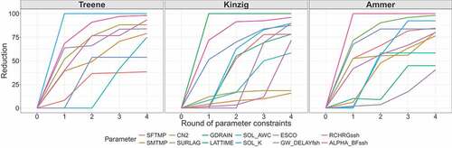
Next, model parameters were constrained separately for each catchment. In the Treene catchment, four model parameters and in the two other catchments only two model parameters were removed. Table 2 shows the reduction of the parameter range at the end of all model simulations in comparison to LHinitial. In the Treene and Kinzig catchments the parameter ranges were reduced to at least 75% for six parameters and in the Ammer catchment for seven parameters.

Table 2. Parameter constraints in the three catchments. The reduction of the parameter range is presented in %. 0% means that the parameter is not changed, × means that the parameter is not considered in LHconstrain and its initial value is kept. The constrained parameter ranges are denoted in brackets (min, max).

Abbreviation	Treene		Kinzig		Ammer
	%	Range	%	Range	%	Range
SFTMP	38	(–0.81, 2.27)	78	(–2.4, – 1.31)	85	(–2.24, – 1.47)
SMTMP	79	(1.28, 2.33)	16	(–2.17, 2.04)	76	(1.32, 2.5)
CN2	88	(2.62, 4.99)	19	(–11.3, 5)	81	(–14.5, – 10.6)
SURLAG	×		×		98	(0.8, 0.86)
LATTIME	×		78	(0.3, 2)	45	(1, 5.3)
GDRAIN	×		×		×
SOL_AWC	75	(0.07, 0.1)	58	(–0.01, 0.04)	58	(–0.02, 0.03)
SOL_K	×		90	(0.5, 0.76)	92	(0.5, 0.69)
ESCO	54	(0.2, 0.57)	88	(0.2, 0.3)	84	(0.87, 1)
GW_DELAYfsh	84	(32.2, 40.1)	90	(1, 5.9)	40	(18.2, 47.4)
RCHRGssh	93	(0.44, 0.48)	72	(0.63, 0.8)	80	(0.2, 0.32)
ALPHA_BFssh	98	(0.002, 0.006)	96	(0.001, 0.009)	×

Figure 3 shows how the parameter ranges were constrained within the four rounds of model simulations. Some ranges which were not reduced in the first round were constrained later. A reduction of the range for the most dominant parameters reduced the impact of parameter variations within the constrained range. Due to that, other model parameters with their initial parameter ranges became relevant.

Figure 3. Reduction of parameter ranges in % for model simulations in the different rounds of parameter constraints. A reduction of 100% means that the parameter was removed from the parameter sampling after the initial simulation round due to a low relevance.

4.3 Parameter identifiability plots for constrained parameter ranges

In the final parameter identifiability plots, both, the selection of relevant model parameters and constrained ranges were different between the catchments (Fig. 4). Overall, in the reduced parameter space, the trade-off between performance criteria was higher and thus more contrasting results were obtained as for LHinitial. This can be explained from the methodological approach. After constraining model parameters for a given performance criterion, a different criterion could be relevant in the reduced range. The reduction of the parameter space made model parameters more insensitive in the constrained parameter range. In this case, these parameters were well identified and a more precise identification of this parameter could not be achieved under consideration of the multiple performance criteria.

Figure 4. Presentation of appropriate parameter values for twelve model parameters in the three catchments using final constrained parameter ranges. See Fig. 2 for explanation. [Colour figure available in online version only.].

In Fig. 4, we show appropriate parameter values after four rounds of parameter constraints (reduction of the parameter ranges). The more the parameter ranges are reduced, the better the parameter is identified. But on the other hand, it is also more difficult to reduce the parameter range further. For example: In the case of ESCO we initially used a parameter range from 0.2 to 1. Due to parameter constraints the range of ESCO is reduced in all three catchments. A further reduction would sacrifice model performance because some criteria have the best values for high and other for low values of ESCO. A more precise identification is not possible for this parameter. In this context, it has to be mentioned that both SOL_AWC and ESCO are soil parameters. Soil parameters are always impacted by different processes, i.e. infiltration, lateral flow, evaporation etc, which are captured by different performance criteria. The contrast in the parameter values means that for one process a high parameter values would be good, for a second process a low parameter value. To represent both processes adequately, parameter ranges may not be further reduced.

Figure 5 shows the optimal parameter values for each performance criterion after the last rounds of parameter constraints separately for the three catchments. For some parameters, their values highly vary among the catchments while the variability is low among the 10 performance criteria, e.g. for CN2, ESCO or RCHRGssh. In these cases, the four rounds of parameter constraints lead to precise identification of parameter values. In other cases, the parameter identifiability is different. For instance, while GW_DELAYfsh is precisely identified in the Kinzig catchment, the variability is still high among the 10 performance criteria in the Ammer catchment.

Figure 5. Optimum parameter values for the 10 performance criteria separately for each catchment as detected in the simulation with the final constrained parameter ranges. The x-axes are adapted to the optimum parameter values and do not represent the full parameter range.

4.4 Impact of parameter constraints on model performance

To evaluate the impact of constrained model parameters, values for the 10 performance criteria were compared between the 2000 simulations of LHinitial and the consecutive reduction of the parameter ranges (LHconstrain) to see how model performance changed due to reduced parameter ranges, both for calibration and validation periods (Fig. 6).

Figure 6. Comparison of performance criteria between model simulations based on initial Latin hypercube sampling (IC: calibration and IV: validation period) and step-wise rounds of constrained parameter ranges (C1–C4: calibration and V1–V1: validation) for all three catchments for the validation period. The different simulation rounds are shaded in grey. The horizontal black line shows optimal value of performance criteria.

In the Treene catchment, all criteria were largely improved for the calibration period. Very poor performing model simulations in terms of NSE and KGE were frequent in LHinitial but did not occur in LHconstrain. Moreover, the variability between the values of the performance criteria was reduced. There is a trade-off between the last two simulation rounds. The overall model performance is better in the fourth round compared to the third round, but this is not valid for all performance criteria. In the Kinzig catchment, the model performance was improved for most of the performance criteria. In particular, performance of NSE, KGE_r and RSR for high, mid and very low flows was improved. In the Ammer catchment, all performance criteria were overall improved after constraining the parameter ranges. The largest improvement was detected here for KGE_beta, RSR for mid, low and very low flows. For all catchments, the model performance was similarly improved also for the validation period.

To summarize the changes in model performance between the initial simulation round and the final parameter constraints, the median values among all model simulations between LHinitial and LHconstrain were compared in Fig. 7 for calibration and validation period. Five contrasting performance criteria (NSE, KGE, KGE_r, RSR for high and very low flows) were improved in all catchments for both periods. The largest improvements were found for Treene and Ammer catchment. In particular, RSR for high, mid and low flows performed better. Thus, the refinement of a parameter ranges can improve all parts of the hydrograph.

Figure 7. Changes in median in the values of performance criteria for the 2000 model simulations of LHinitial and the final simulations of LHconstrain for the calibration and validation period. Please note that the optimal values vary between the performance criteria. The black horizontal line shows the optimal value of the performance criteria. Tr: Treene; Ki: Kinzig; Am: Ammer; followed by C for calibration and V for validation.

4.5 Uncertainty in modelled discharges between initial and final parameter ranges

The modelled discharge has a lower variability and performs overall better in LHconstrain compared to LHinitial (Fig. 8). This is the case for the Treene lowland catchment where high variability in modelled discharge under low flow conditions is largely reduced in LHconstrain. Also in the two other catchments, the uncertainty in modelled discharge is in particular reduced for low flows, but to a lower extent compared to the Treene catchments. For a better interpretation of low flows, the reader is referred to the same figure with a log-scale in the Supplementary material.

Figure 8. Comparison of simulated discharge time series using the model simulations with the initial parameter ranges (LHinitial) and the final parameter constraints (LHconstrain) with the observed discharge time series. For both simulations, the 5% and 95% of the 2000 simulations are shown in separate subplots for the three catchments.

4.6 Parameter space

The averages of the minimum Euclidean distances between all parameter sampling approaches (LHinitial, LHinitial with 5000 runs, LHconstrain for all three catchments) were shown in Fig. 9. The minimum Euclidean distance was largest for LHinitial. The largest reduction in the Euclidean distance was achieved in reducing the number of parameters. Thus, the lowest number of parameters in the Treene led to the smallest Euclidean distance. In addition, also a reduction of the parameter space reduced the Euclidean distance stronger than an increase in model simulations, e.g. a comparison of the first (Ki.1) with the last round of parameter constraints (Ki.4). Furthermore, the Euclidean distance also varied between the two other catchments with an identical number of parameters due to the differences in the parameter ranges. Each reduction of the parameter range reduced the parameter space. Moreover, the variability between the boxplots was also lower in the final simulation round.

Figure 9. Average minimum Euclidean distances among parameter sets in the parameter space. Each catchment is shown in different colours. Tr: Treene; Ki: Kinzig; Am: Ammer. The number denotes the rounds of parameter constraints.

5 Discussion

5.1 Differences and similarities in parameter identifiability using multiple performance criteria

Parameter identifiability plots for different performance criteria show how strongly the identification of behavioural parameter values depends on the selection of performance criteria (Wagener et al. 2003, Fenicia et al. 2008, Pfannerstill et al. 2014b). All selected criteria are relevant for certain parameters at least in one of the catchments. This implies that none of the criteria could be neglected and that it is required to investigate the parameter identifiability for different criteria. A large benefit of our approach is that it becomes apparent which criteria reduce which parameter to which values. Moreover, the behavioural ranges can be compared between the 10 criteria.

The handling of contrasting results of behavioural parameter values for different performance criteria needs to be considered in more detail. It is required to prioritize the selection of performance criteria to ensure the identification of behavioural parameter values. A strong relationship between a parameter and a performance criterion facilitates a precise parameter identification (Guse et al. 2017). In particular, complex models such as the SWAT model often contain parameters with a low identifiability (van Werkhoven et al. 2009) and it is therefore more difficult to constrain their parameters. In particular, the identifiability of model parameters that correspond to several processes or that are related to interacting processes is lower such as it is the case for evaporation or soil parameters. By repeating model simulations in several steps, it is possible to reduce at first the ranges of parameters which are clearly identifiable. After identifying these parameter values, also the parameters regulating complex model behaviour are constrained. Model parameters of moderate relevance are only reduced after constraining other more dominant parameters in the first simulations. This is demonstrated in this study by several rounds of parameter constraints.

If two parameters are correlated, it is expected that the ranges of the more dominant parameter are at first reduced, while the ranges of the other parameters remain constant. Since our methodological approach is applied in four rounds of parameter constraints, the relevance of correlated parameters might change and also a previously unidentifiable parameter might become relevant and could be identified.

5.2 Benefit of constraining model parameters

Smaller parameter ranges due to parameter constraints also reduce their sensitivity. In the optimal case, the analysis of parameter identifiability plots constrain parameters such that only a small value range remains. Precise parameter identifiability reduces equifinality since the impact of different parameter values within this small range is low (Cibin et al. 2014). A model parameter which is unidentifiable for the 10 contrasting performance criteria can be assumed to be of low relevance in controlling the hydrological system in this catchment. This is in particular the case if the corresponding process is also of low relevance. Keeping a parameter value at the default value is an important result, since it reduces the number of parameters in the parameter sampling and thus the overall parameter space. The increase of identifiability due to reduction of parameter space is in line with outcomes by Wagener (2007) and Pokhrel et al. (2008).

The refinement of the parameter space results in smaller distances between two parameter sets in the parameter space. Based on this, more behavioural parameter combinations are selected. In other words, a wide range for even a few parameters can lead to a large number of model runs with poor performance. Thus, it is demonstrated how a careful preselection of the parameter space helps in identifying parameter values accurately. This increases also the possibility to detect parameter sets which are acceptable for multiple performance criteria. The number of acceptable parameter sets for a certain performance criterion is higher after the refinement of the parameter ranges such as for NSE and KGE. Extremely poor model performance is avoided by constraining parameter ranges, since too unrealistic parameter combinations are removed.

It is more useful to select the parameter space distance than the number of model simulations as a criteria for a sufficient number of model simulations. More studies using different models and a large set of catchments are required in future to define a threshold for a maximum distance in the parameter space that should not be exceeded on average. For a defined average parameter space distance it would then be possible to assess the number of required model simulations for a given number of parameters.

This study was mainly focused on parameter identification, but certainly, model results are also affected by different sources of uncertainty. The impact of model parameters depends among other factors on how the uncertainty source influences the associated process. In this context, we expect that a surface runoff parameter is influenced in particular by precipitation data uncertainty. In contrast, the available soil water capacity SOL_AWC is more affected by the selection of the soil map in the model set-up.

A next step could be to apply this method to a large set of catchments. Then, parameter constraints can be related to catchment characteristics. In the best case, some of the SWAT model parameters could be identified based on catchment characteristics as a background for improving the simulations of ungauged basins.

5.3 Spatial variability in improving model performance

Our study shows that the reduction of parameter space and the improvement of model performance is greater in the catchments with low process complexity. In particular, Treene and Ammer catchments are strongly dominated by groundwater or surface and snow processes, respectively. This allows a clearer parameter value identification than in the mid-range catchments which are characterized by an overlay of different dominant processes at the same time and for the same flow conditions (Guse et al. 2019).

The model performance varied between the catchments. These differences in the model performance in the three catchments agree with the suggestion of Seibert et al. (2018) to differentiate between upper and lower benchmarks among catchments. In comparing model performance between the catchments, it needs to be considered that the model performance also depends among others on input data such as precipitation. The more complex interaction between snow and rain phases due to the higher altitude of the Ammer catchment results in a worse model performance than in the two other catchments with low snow relevance and less spatial heterogeneity of rainfall. It was not our intention to optimize a parameter to unrealistic values to achieve better values of the performance criteria. As suggested by Wagener et al. (2001), we restricted our approach to realistic parameter ranges. This highlights the necessity to make use of all data and knowledge available for a catchment to carefully select appropriate performance criteria and appropriate parameters (ranges) (Arnold et al., 2015).

The improvement of model performance is in agreement with other studies that used constraints for performance criteria to improve the hydrological consistency of model results (Shamir et al. 2005, Yadav et al. 2007, Nalbantis et al. 2011, Yen et al. 2014, Pfannerstill et al. 2017). Based on former studies with the SWAT model and the results from this study, the performance criteria are characterized in how they are related to the parts of the hydrograph in different hydrological components and the SWAT model parameters. Table 3 allows the selection of performance criteria for minimizing specific model errors and for targeting selected parts of the hydrograph. It also gives an indication which performance criteria is most relevant in which region and for which SWAT model parameter. This represents valuable information for improving model calibration.

Table 3. Relationship of performance criteria, part of hydrograph, hydrological components and SWAT model parameters.

Performance criteria	Considered model error	Part of hydrograph	Hydrological component	Model parameter
NSE	Higher weights on variability than on correlation and bias	Focus on high flows	Fast runoff components	Catchment-specific
KGE	Same weights on variability, bias, correlation	Entire hydrograph	All	Catchment-specific
KGE_alpha	Variability	Variability	Dominant runoff component	Catchment-specific
KGE_beta	Bias	Water balance	Soil, evaporation	ESCO, SOL_AWC
KGE_r	Correlation	Timing	Several processes	SMTMP, SURLAG
RSR for very high flows	Very high flows	Very high flows	Surface runoff	CN2
RSR for high flows	High flows	High flows	Fast runoff components	Catchment-specific
RSR for mid flows	Mid flows	Mid flows	Soil, evaporation	ESCO, SOL_AWC
RSR for low flows	Low flows	Low flows	Soil, groundwater flow	Catchment-specific
RSR for very low flows	Very low flows	Very low flows	Baseflow	ALPHA_BFssh

This result demonstrates the benefit of constraining model parameters first. We see our approach as a study before carrying out a model calibration. The reduction of the parameter ranges reduces the parameter space and allows thus a more precise parameter sampling independent from the sampling method. The constrained parameter ranges enable a targeted and more effective multi-objective calibration to detect behavioural model runs for scenario simulations (Efstratiadis and Koutsoyiannis 2010). Targeted multi-objective calibration was not in the focus of this study, since a selection of one or a few best model runs always depends on the study goal due to the trade-off in optimizing different performance criteria (Kiesel et al. 2017).

6 Conclusions

In this study, a method is presented to constrain model parameters and to systematically increase parameter identifiability. It is investigated how parameter identifiability vary using multiple performance criteria and between different catchments. In the case of high parameter identifiability, parameter are constrained to small ranges. Following on this, model simulations are repeated with the reduced parameter ranges to improve parameter identifiability and model performance successively.

The main outcomes are:

1. Parameter identifiability plots with multiple performance criteria lead to reliable estimates of reasonable parameter ranges. Most of the parameters are constrained to smaller ranges in these catchments. These parameter identifiability plots partly lead to contradictive interpretations of good parameter values due to a trade-off in optimising different performance criteria. This can be explained by different processes that are related to these parameters.

2. The trade-off between different performance criteria is reduced by consecutive rounds of parameter refinements and repetitions of model simulations. Model parameters of moderate relevance are identified in a later round, after constraining the dominant model parameters to smaller ranges.

3. The identifiability of a model parameter varies between the catchments in the case of different relevance of the associated process.

4. Overall, a refinement of the parameter space improves the model performance and leads to a high amount of good performing model simulations.

These analyses show that contrasting performance criteria are required for an accurate parameter value identification as a requirement for reliable hydrological modelling and that a reduction of the parameter space improves the model performance.

Acknowledgements

For the discharge data, we thank Schleswig-Holstein Agency for Coastal Defence, National Park and Marine Conservation of Schleswig-Holstein (LKN-SH), the Hessian Agency for Nature Conservation, Environment and Geology (HLNUG) and the Bavarian Agency for Environment (LfU). We would like to thank the community of the open source software R. Finally, we thank the Associate Editor, Andreas Efstratiadis, and two anonymous reviewers for very constructive comments to improve our manuscript.

Disclosure Statement

No potential conflict of interest was reported by the authors.

Supplementary material

Supplemental data for this article can be accessed here.

Additional information

Funding

We thank the German Research Foundation (DFG, Deutsche Forschungsgemeinschaft) for financial support (Project GU 1466/1-1 Hydrological consistency in modelling). JK acknowledges funding through the “GLANCE” project (Global change effects on river ecosystems; 01LN1320A) supported by the German Federal Ministry of Education and Research (BMBF).

References

- Abebe, N., Ogden, F., and Pradhan, N., 2010. Sensitivity and uncertainty analysis of the conceptual HBV rainfall-runoff model: implications for parameter estimation. Journal of Hydrology, 389, 301–310. doi:10.1016/j.jhydrol.2010.06.007
- Arnold, J., et al., 1998. Large area hydrologic modeling and assessment part I: model development. Journal of the American Water Resources Association, 34, 73–89. doi:10.1111/jawr.1998.34.issue-1
- Arnold, J., et al., 2015. Hydrological processes and model representation: impact of soft data on calibration. Transactions of the ASABE, 58, 1637–1660. doi:10.13031/trans.58.10726
- Bekele, E.G. and Nicklow, J.W., 2007. Multi-objective automatic calibration of SWAT using NSGA-II. Journal of Hydrology, 341, 165–176. doi:10.1016/j.jhydrol.2007.05.014
- Boyle, D., Gupta, H., and Sorooshian, S., 2000. Toward improved calibration of hydrologic models: combining the strengths of manual and automatic methods. Water Resources Research, 36 (12), 3663–3674. doi:10.1029/2000WR900207
- Boyle, D.P., et al., 2001. Toward improved streamflow forecasts: value of semidistributed modeling. Water Resources Research, 37 (11), 2749–2759. doi:10.1029/2000WR000207
- Cibin, R., et al., 2014. Application of distributed hydrological models for predictions in ungauged basins: a method to quantify predictive uncertainty. Hydrological Processes, 28, 2033–2045. doi:10.1002/hyp.9721
- Cibin, R., Sudheer, K.P., and Chaubey, I., 2010. Sensitivity and identifiability of stream flow generation parameters of the SWAT model. Hydrological Processes, 24, 1133–1148. doi:10.1002/hyp.v24:9
- Efstratiadis, A. and Koutsoyiannis, D., 2010. One decade of multi-objective calibration approaches in hydrological modelling: a review. Hydrological Sciences Journal, 55, 58–78. doi:10.1080/02626660903526292
- Fenicia, F., McDonnell, J.J., and Savenije, H.H., 2008. Learning from model improvement: on the contribution of complementary data to process understanding. Water Resources Research, 44, W06419. doi:10.1029/2007WR006386
- Gharari, S., et al., 2014. A constraint-based search algorithm for parameter identification of environmental models. Hydrology and Earth System Science, 18, 4861–4870. doi:10.5194/hess-18-4861-2014
- Gupta, H., Sorooshian, S., and Yapo, P., 1998. Toward improved calibration of hydrologic models: combining the strengths of manual and automatic methods. Water Resources Research, 34 (4), 751–763. doi:10.1029/97WR03495
- Gupta, H.V., et al., 2009. Decomposition of the mean squared error and NSE performance criteria: implications for improving hydrological modelling. Journal of Hydrology, 377, 80–91. doi:10.1016/j.jhydrol.2009.08.003
- Guse, B., et al., 2016. On characterizing the temporal dominance patterns of model parameters and processes. Hydrological Processes, 30 (13), 2255–2270. doi:10.1002/hyp.10764
- Guse, B., et al., 2017. Identifying the connective strength between model parameters and performance criteria. Hydrology and Earth System Science, 21, 5663–5679. doi:10.5194/hess-21-5663-2017
- Guse, B., et al., 2019. Analysing spatio-temporal process and parameter dynamics in models to characterise contrasting catchments. Journal of Hydrology, 507, 863–874. doi:10.1016/j.jhydrol.2018.12.050
- Guse, B., Reusser, D.E., and Fohrer, N., 2014. How to improve the representation of hydrological processes in SWAT for a lowland catchment - temporal analysis of parameter sensitivity and model performance. Hydrological Processes, 28, 2651–2670. doi:10.1002/hyp.977
- Hogue, T.S., Gupta, H., and Sorooshian, S., 2006. A user-friendly approach to parameter estimation in hydrologic models. Journal of Hydrology, 320, 202–217. doi:10.1016/j.jhydrol.2005.07.009
- Kakouei, K., et al., 2018. Projected effects of climate-change-induced flow alterations on stream macroinvertebrate abundances. Ecology and Evolution, 8 (6), 3393–3409. doi:10.1002/ece3.3907
- Kelleher, C., et al., 2013. Identifiability of transient storage model parameters along a mountain stream. Water Resources Research, 49 (9), 5290–5306. doi:10.1002/wrcr.20413
- Kiesel, J., et al., 2017. Improving hydrological model optimization for riverine species. Ecological Indicators, 80, 376–385. doi:10.1016/j.ecolind.2017.04.032
- Kiesel, J., et al., 2019. Climate change impacts on ecological relevant hydrological indicators in three catchment in three European ecoregions. Ecological Engineering, 127, 404–416. doi:10.1016/j.ecoleng.2018.12.019
- Kling, H., Fuchs, M., and Paulin, M., 2012. Runoff conditions in the Upper Danube basin under an ensemble of climate change scenarios. Journal of Hydrology, 424–425, 264–277. doi:10.1016/j.jhydrol.2012.01.011
- Kumar, R., Samaniego, L., and Attinger, S., 2010. The effects of spatial discretization and model parameterization on the prediction of extreme runoff characteristics. Journal of Hydrology, 392, 54–69. doi:10.1016/j.jhydrol.2010.07.047
- Madsen, H., 2000. Automatic calibration of a conceptual rainfall-runoff model using multiple objectives. Journal of Hydrology, 235, 276–288. doi:10.1016/S0022-1694(00)00279-1
- Martinez, G.F. and Gupta, H.V., 2011. Hydrologic consistency as a basis for assessing complexity of monthly water balance models for the continental united states. Water Resources Research, 47, W12540. doi:10.1029/2011WR011229
- Moriasi, D.N., et al., 2007. Model evaluation guidelines for systematic quantification of accuracy in watershed simulations. Transactions of the ASABE, 50 (3), 885–900. doi:10.13031/2013.23153
- Nalbantis, I., et al., 2011. Holistic versus monomeric strategies for hydrological modelling of human-modified hydrosystems. Hydrology and Earth System Science, 15, 743–758. doi:10.5194/hess-15-743-2011
- Nash, J.E. and Sutcliffe, J.V., 1970. River flow forecasting through conceptual models: part I - a discussion of principles. Journal of Hydrology, 10, 282–290. doi:10.1016/0022-1694(70)90255-6
- Neitsch, S., et al., 2011. Soil and Water Assessment Tool - theoretical documentation version 2009. Texas Water Resources Institute Technical Report, 406.
- Pechlivanidis, I.G., et al., 2014. Use of entropy-based metric in multiobjective calibration to improve model performance. Water Resources Research, 50, 8066–8083. doi:10.1002/2013WR014537
- Pfannerstill, M., et al., 2015. Process verification of a hydrological model using a temporal parameter sensitivity analysis. Hydrology and Earth System Science, 19, 4365–4376. doi:10.5194/hess-19-4365-2015
- Pfannerstill, M., et al., 2017. How to constrain multi-objective calibrations of the SWAT model using water balance components. Journal of the American Water Resources Association, 53 (3), 532–546. doi:10.1111/1752-1688.12524
- Pfannerstill, M., Guse, B., and Fohrer, N., 2014a. A multi-storage groundwater concept for the SWAT model to emphasize nonlinear groundwater dynamics in lowland catchments. Hydrological Processes, 28, 5599–5612. doi:10.1002/hyp.10062
- Pfannerstill, M., Guse, B., and Fohrer, N., 2014b. Smart low flow signature metrics for an improved overall performance evaluation of hydrological models. Journal of Hydrology, 510, 447–458. doi:10.1016/j.jhydrol.2013.12.044
- Pokhrel, P., Gupta, H., and Wagener, T., 2008. A spatial regularization approach to parameter estimation for a distributed watershed model. Water Resources Research, 44, W12419. doi:10.1029/2007WR006615
- Pokhrel, P., Yilmaz, K.K., and Gupta, H.V., 2012. Multiple-criteria calibration of a distributed watershed model using spatial regularization and response signatures. Journal of Hydrology, 418–419, 49–60. doi:10.1016/j.jhydrol.2008.12.004
- Reusser, D., et al., 2009. Analysing the temporal dynamics of model performance for hydrological models. Hydrology and Earth System Science, 13, 999–1018. doi:10.5194/hess-13-999-2009
- Seibert, J., et al., 2018. Upper and lower benchmarks in hydrological modelling. Hydrological Processes, 32, 1120–1125. doi:10.1002/hyp.11476
- Shamir, E., et al., 2005. Application of temporal streamflow descriptors in hydrologic model parameter estimation. Water Resources Research, 41, W06021. doi:10.1029/2004WR003409
- Shin, M.J., et al., 2015. A review of foundational methods for checking the structural identifiability of models: results for rainfall-runoff. Journal of Hydrology, 520, 1–16. doi:10.1016/j.jhydrol.2014.11.040
- Soetaert, K. and Petzoldt, T., 2010. Inverse modelling, senstivity and Monte Carlo analysis in R using package FME. Journal of Statistical Software, 33 (3), 1–28. 10.1.1.160.5179. doi:10.18637/jss.v033.i03
- Van Griensven, A., et al., 2006. A global sensitivity analysis tool for the parameters of multi-variable catchment models. Journal of Hydrology, 324, 10–23. doi:10.1016/j.jhydrol.2005.09.008
- van Werkhoven, K., et al., 2009. Sensitivity-guided reduction of parametric dimensionality for multi-objective calibration of watershed models. Advances in Water Resources, 32 (8), 1154–1169. doi:10.1016/j.advwatres.2009.03.002
- Wagener, T., et al., 2001. A framework for development and application of hydrological models. Hydrology and Earth System Science, 5 (1), 13–26. doi:10.5194/hess-5-13-2001
- Wagener, T., et al., 2003. Towards reduced uncertainty in conceptual rainfall-runoff modelling: dynamic identifiability analysis. Hydrological Processes, 17, 455–476. doi:10.1002/()1099-1085
- Wagener, T., 2007. Can we model the hydrological impacts of environmental change? Hydrological Processes, 21, 3233–3236. doi:10.1002/()1099-1085
- Wagener, T. and Kollat, J., 2007. Numerical and visual evaluation of hydrological and environmental models using the Monte Carlo analysis toolbox. Environmental Modelling & Software, 22, 1021–1033. doi:10.1016/j.envsoft.2006.06.017
- Westerberg, I.K., et al., 2014. Regional water balance modelling using flow-duration curves with observational uncertainties. Hydrology and Earth System Science, 18, 2993–3013. doi:10.5194/hess-18-2993-2014
- Yadav, M., Wagener, T., and Gupta, H., 2007. Regionalization of constraints on expected watershed response behavior for improved predictions in ungauged basins. Advances in Water Resources, 30, 1756–1774. doi:10.1016/j.advwatres.2007.01.005
- Yen, H., et al., 2014. The role of interior watershed processes in improving parameter estimation and performance of watershed models. Journal of Environmental Quality, 43, 1601–1613. doi:10.2134/jeq2013.03.0110
- Yilmaz, K.K., Gupta, H., and Wagener, T., 2008. A process-based diagnostic approach to model evaluation: application to the NWS distributed hydrologic model. Water Resources Research, 44, W09417. doi:10.1029/2007WR006716
- Zhang, H., et al., 2011. Multi-period calibration of a semi-distributed hydrological model based on hydroclimatic clustering. Advances in Water Resources, 34, 1292–1303. doi:10.1016/j.advwatres.2011.06.005
- Zink, M., et al., 2018. Conditioning a hydrologic model using patterns of remotely sensed land surface temperature. Water Resources Research, 54, 2976–2998. doi:10.1002/2017WR021346