Blunt extension of discrete universal multifractal cascades: development and application to downscaling

ABSTRACT

Scale issues are ubiquitous in geosciences. Because of their simplicity and intuitiveness, and despite strong limitations, notably its non-stationarity features, discrete random multiplicative cascade processes are very often used to address these scale issues. A novel approach based on the parsimonious framework of Universal Multifractals (UM) is introduced to tackle this issue while preserving the simple structure of discrete cascades. It basically consists in smoothing at each cascade step the random multiplicative increments with the help of a geometric interpolation over a moving window. The window size enables to introduce non-conservativeness in the simulated fields. It is established theoretically,] and numerically confirmed, that the simulated fields also exhibit a multifractal behaviour with expected features. It is shown that such an approach remains valid over a limited range of UM parameters. Finally, we test downscaling of rainfall fields with the help of this blunt discrete cascade process, and we discuss challenges for future developments.

KEYWORDS:

• multifractals
• discrete random multiplicative cascades
• downscaling
• rainfall

Editor A. Castellarin Associate editor E. Volpi

1 Introduction

Scale issues are ubiquitous in the geosciences and particularly in the atmospheric sciences, both theoretically and practically. Indeed, they are intrinsically related to the need to better understand the underlying processes and notably the consequences of scale invariance of the Navier-Stokes equations. This has led to the emergence of cascade approaches (Kolmogorov 1941) to model turbulence. Since turbulence is considered to generate and drive spatio-temporal variability in the atmosphere and notably clouds, such scale-invariant features are also expected to be transferred to the unknown equations governing other fields such as rainfall (Schertzer and Lovejoy 1987, Hubert 2001). They are also required from a practical point of view with very common issues such as how to address the spatio-temporal gap of the observation scales of two measuring devices that need to be compared or how to downscale a field from an available coarse resolution to a needed higher resolution.

In such processes, an average intensity over a large-scale structure is iteratively distributed in space and time to smaller-scale structures. Schertzer and Lovejoy (1987) argued on the necessity to go beyond additive processes as well as beyond discrete (in scale) cascades to respect the nonlinearity, continuous translation and scale invariances of the generating equations. They therefore introduced continuous (in scale) cascades. For the pedagogical (although unphysical) example of discrete cascades, a structure is divided into ${\lambda }_1^d$ sub-structures where d is the dimension of the embedding space (d = 1 in 1D and d = 2 in 2D). Usually ${\lambda }_1=2$ i.e. time steps are simply divided in 2, and pixels in 4. The intensity affected to a sub-structure is the intensity of the parent structure multiplied by a random increment. Then, the process is iteratively repeated on each of the sub-structures. The process is scale invariant in the sense that the way structures are divided into sub-structures and the probability distribution of the random multiplicative increments are the same at each cascade step. More details are provided in Section 2. Such scale invariance is usually valid only on a limited range of scales that should be determined through data analysis.

Discrete random multiplicative cascades have been extensively used to model rainfall. For example, they have been used in a spatio-temporal context with log-normal distributions for the increments and in combination with a β-model to improve representation of zeros (Gupta and Waymire 1993, Over and Gupta 1996). Olsson. (1998) developed an approach in which zeros are introduced within a micro-canonical cascade process in a way that is tailored to the simulated intensity. Micro-canonical means that intensity is preserved exactly through each cascade step and not only on average, as is a canonical cascade, which enables one to introduce more variability. Gires et al. (2013) also developed a model to account better for the zeros of rainfall by adding the possibility of the process to be set to zero at each cascade step if the intensity is not great enough. Menabde and Sivapalan (2000) used bounded discrete cascades with Levy-stable distributions. Gaume et al. (2007) used a canonical log-Poisson model and a micro-canonical model with uniform distribution of the increments’ distribution for hydrological purposes. Licznar et al. (2011) carried out an extensive comparison of six models, mainly relying on log-normal distribution and with numerous parameters (up to 11). Müller and Haberlandt (2018) developed an approach in which the distribution implemented varies according to the cascade step. Rupp et al. (2012) explored the use of log-normal models to simulate rainfall spatial variability.

Such a seemingly simple and intuitive process enables one to parsimoniously (and partly) reproduce complex patterns exhibiting extreme variability and intermittence over a wide range of spatio-temporal scales. This is the reason for their ‘success’, despite their strong, aforementioned limitations. A visual drawback of these limitations is the existence of sharp transitions between areas/periods of the generated fields, notably unrealistic square structures in 2D. Some of the authors cited above have acknowledged these limitations in their discussions but did not attempt to deal with them.

In this paper, we present an innovative way to lessen some limitations of discrete random multiplicative cascades and to develop a rather straightforward downscaling application. We basically simply suggest to interpolate at each cascade step the random multiplicative increments and hence avoid the sharp transitions within the generated fields.

The paper is organized as follows. First, we present the framework of discrete cascades and universal multifractals which we will use (see Schertzer and Tchiguirinskaia 2018, for a recent review, as well as extensions to – continuous in scale – multifractals operating on vector fields), along with a description of the limitations of discrete cascades (Section 2). Then, the approach introduced herein to improve discrete cascades is progressively presented and validated in Section 4. Finally, the suggested framework is applied to downscaling rainfall time series and maps with implementation and validation (Section 5).

2 Universal multifractals (UM) discrete cascade and position of the problem

2.1 UM discrete cascades

Let us consider a field $B_{\lambda }$ at a resolution $\lambda$ defined as the ratio between the outer scale L and the observation scale l ($\lambda =L/l$). In practice, a field is usually measured at a maximum resolution (${\lambda }_{\mathrm{m}\mathrm{a}\mathrm{x}}$) and up-scaled from it at lower resolutions by averaging over adjacent times steps or pixels. Such a process does not enable us to retrieve the exact values of the increments used for generating a field (see below), and the interested reader is referred to Schertzer and Lovejoy (1987) for complete discussion of the difference between what is denoted in the literature a bare (obtained during the generation) and dressed (obtained after up-scaling from the maximum resolution) fields. For multifractal fields, the moment of order q of the field is a power law related to the resolution:

(1) $⟨B_{\lambda }^q⟩\approx {\lambda }^{K\left(q\right)}$(1)

where $K\left(q\right)$ is the scaling moment function that fully characterizes the variability across scales of the field. In the specific framework of UM (Schertzer and Lovejoy 1987, 1997), towards which multiplicative cascades processes converge, $K\left(q\right)$ for conservative fields is defined with the help of only two parameters with physical interpretation:

• $C_1$, the mean intermittency co-dimension, which measures the clustering of the (average) intensity at smaller and smaller scales. $C_1=0$ for a homogeneous field;

• $\alpha$, the multifractality index ($0\le \alpha \le 2$), which measures the clustering variability with regards to the intensity level.

For UM, we have:

(2) $K\left(q\right)=\frac{C_1}{\alpha -1}\left(q^{\alpha }-q\right)$(2)

A multifractal analysis consists of checking that these features are indeed observed. The quality of the scaling can be assessed with the help of trace moment (TM) analysis which basically consists of plotting in Equation (1) log-log. Straight lines should be retrieved and the slope gives $K\left(q\right)$. The coefficient of determination $r^2$ for $q=1.5$ is used in this paper as an indicator of the quality of the scaling. The double trace moment (DTM) technique is tailored for UM fields and enables robust estimation of UM parameters (Lavallée et al. 1993). DTM was used herein for this purpose.

In the previous case, the average intensity is conserved across scales and the field is said to be conservative. In general, for multiplicative processes, conservation refers to the fact that a given statistic – usually the mean – is strictly independent of scale. Fields which do not exhibit such features are said to be non-conservative and an additional parameter called the non-conservation parameter and denoted H needs to be introduced, where $H=0$ for conservative fields; it can be either positive or negative. More physically, greater values H correspond to stronger correlations within the studied field. H is typically between 0 and 1 for geophysical fields.

In such a framework, a non-conservative field ($B_{\lambda }^{\prime }$) can be decomposed as follows:

(3) $B_{\lambda }^{\prime }\approx B_{\lambda }{\lambda }^{-H}$(3)

where $B_{\lambda }^{\text{boxempty}}$ is a conservative field and the portion corresponding to the variations of the average field has been separated. In such a case, the slope β of the spectra $E\left(k\right)$ (where k is the wave number):

(4) $E\left(k\right)\approx k^{-\beta }$(4)

is related to H as follows:

(5) $\beta =1+2H-K\left(2\right)$(5)

The value of H is actually estimated with the help of this equation after carrying out a spectral analysis, which also gives an indication of the quality of the scaling (Lavallée et al. 1993).

It is possible to generate UM fields with the help of discrete multiplicative cascades as described in the introduction. The process is illustrated with three steps in Fig. 1. We start with a large-scale structure, with a given intensity $B_0$. After n steps, the resolution is ${\lambda }_1^n={\lambda }_n$, and a value $B_{n,i}$ (i ranging from 1 to $2^n$) of the field is the product of the increments associated with all its successive parent structures:

(6) $B_{n,i}=B_0\prod _{s=1}^n\left(b_s\right)$(6)

Figure 1. Illustration of a standard discrete multiplicative cascade process with three steps. $B_{n,i}$ are the values of the field after n steps and $b_{n,i}$ are the increments.

where $b_s$ is a realization of the random variable b defining the increments. For UM the random variable of increment b is given by:

(7) $b=\frac{\mathrm{e}\mathrm{x}\mathrm{p}\left[{\left(\frac{C_{1}ln{\lambda }_1}{\left|\alpha -1\right|}\right)}^{1/\alpha }L\left(\alpha \right)\right]}{{\lambda }_1^{\frac{C_1}{\alpha -1}}}$(7)

where $L\left(\alpha \right)$ is an extremal Lévy-stable random variable of index $\alpha$. This is generated with the help of the procedure given by Chambers et al. (1976), and has the following property:

(8) $⟨exp[qL(\alpha )]⟩=exp[q^{\alpha }]$(8)

Combining Equations (7 and 8), we find:

(9) $⟨b^q⟩=\frac{⟨\mathrm{e}\mathrm{x}\mathrm{p}\left[q{\left(\frac{C_1\mathrm{l}\mathrm{n}{\lambda }_1}{\left|\alpha -1\right|}\right)}^{1/\alpha }L\left(\alpha \right)\right]⟩}{{\lambda }_1^{q\frac{C_1}{\alpha -1}}}={\lambda }_1^{\frac{C_1}{\alpha -1}\left(q^{\alpha }-q\right)}$(9)

Finally, given that the increments $b_s$ in Equation (6) are independent and identically distributed, and keeping in mind ${\lambda }_1^n={\lambda }_n$, we can demonstrate that the field simulated is indeed a UM one:

(10) $⟨B_{n,i}^q⟩=B_0^q{⟨b^q⟩}^n={\lambda }_n^{\frac{C_1}{\alpha -1}\left(q^{\alpha }-q\right)}$(10)

2.2 The issue of non-stationarity

Universal multifractal discrete cascades follow Equations (1 and 2). However, they are not stationary in the sense that the correlation between two points does not only depend on the lag between them.

In order to illustrate this issue, let us consider three time steps – $B_{3,3}$, $B_{3,4}$ and $B_{3,5}$ – of the three-step cascade process displayed in Equation (1). We aim to compute the two correlations $⟨B_{3,3}^q{B}_{3,4}^q⟩$ and $⟨B_{3,4}^q{B}_{3,5}^q⟩$, where q is a moment order (the standard correlation is retrieved for $q=1$). The symbol $⟨\text{boxempty}⟩$ refers to the estimation of the mean taken over numerous independent realizations of the process, which then yields an estimate of the expected value of the process. Following Equation (6), these time steps can be written as:

(11) $\begin{array}{ccc}{B}_{3,3}& =& B_{0,1}{b}_{1,1}{b}_{2,2}{b}_{3,3}\\ B_{3,4}& =& B_{0,1}{b}_{1,1}{b}_{2,2}{b}_{3,4}\\ B_{3,5}& =& B_{0,1}{b}_{1,2}{b}_{2,3}{b}_{3,5}\end{array}$(11)

From Equation (11), it is possible to quickly deduce that $B_{3,3}$ and $B_{3,4}$ share two increments (one at level $n=1$ which is $b_{1,1}$, one at level $n=2$ which is $b_{2,2}$ and none at level $n=3$), while $B_{3,4}$ and $B_{3,5}$ share none. This has some consequences when the correlations are computed. Indeed, we obtain:

(12) $\begin{array}{c}⟨B_{3,3}^q{B}_{3,4}^q⟩\\ ⟨B_{3,4}^q{B}_{3,5}^q⟩\end{array}\begin{array}{c}=\\ =\end{array}\begin{array}{c}⟨B_{0,0}^{2q}{b}_{1,1}^{2q}{b}_{2,2}^{2q}{b}_{3,3}^q{b}_{3,4}^q⟩\\ ⟨B_{0,0}^{2q}{b}_{1,1}^q{b}_{2,2}^q{b}_{3,4}^q{b}_{1,2}^q{b}_{2,3}^q{b}_{3,5}^q⟩\end{array}\begin{array}{c}=\\ =\end{array}\begin{array}{c}{B}_{0,0}^{2q}{⟨b^{2q}⟩}^2{⟨b⟩}^{2q}\\ B_{0,0}^{2q}{⟨b⟩}^{6q}\end{array}$(12)

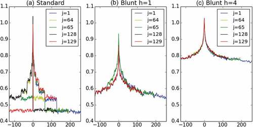
from which it is clear to see that they are not equal in the general case. This simple example illustrates why discrete cascades are not stationary. Such features are also observed on more developed cascades and not considering adjacent time steps. This is studied in Fig. 2. More precisely 10 000 samples of an 8-step discrete cascade with $\alpha =1.6$ and $C_1=0.2$ are generated (hence, time series of length 256 are obtained) and the quantities $⟨B_{8,j}^q{B}_{8,j+t}^q⟩$ are studied for various j and t. Figure 2 displays, for $q=0.5$, $⟨B_{8,j}^q{B}_{8,j+t}^q⟩$ as a function of t for $j=1$, $j=64$ (just before one-quarter of the series, $j=65$ (just after one-quarter of the series), $j=128$ (just before the middle of the series), and $j=129$ (just after the middle of the series). The range of possible values for t will not be the same, which is why the curves are all shifted on Fig. 2. For example, for $j=1$ we have $t\subset \left[0,\dots ,255\right]$, while for $j=128$ we have $t\subset \left[-127,\dots ,128\right]$. The strongly asymmetric behaviour with a transition for $t=0$ is visible for $j=128$ and $j=129$ with standard discrete cascade simulations (Fig. 2(a)). It is also the case, to a smaller extent, for $j=64$ and $j=65$, which was expected since these two time steps share one more increment together ($b_{1,1}$). Such asymmetry illustrates well the strong limitations of discrete cascades due to their non-stationarity. Similar features are obtained with 2D fields, and it is actually the phenomenon that causes the sharp unrealistic square structures obtained in such fields (see Fig. 10 for an illustration).

Figure 2. $⟨B_{8,j}^q{B}_{8,j+t}^q⟩$ as a function of t for $q=0.5$ and various j on 256 time step series simulated with $\alpha =1.6$ and $C_1=0.2$. (a) Standard cascade, (b) blunt cascade with $h=1$, and (c) blunt cascade with $h=4$.

3 Presentation of blunt discrete UM cascades

The aim in this section is to introduce a new model for multiplicative cascades based on a modification of standard UM discrete cascades and characterize its mathematical behaviour. As a consequence, it will be introduced starting from the standard well-known process. The underlying concept is actually rather straightforward and easy.

It can be summarized in three successive steps: (a) present increments at the final resolution; (b) perform a geometrical average with a moving window to replace the increments at each cascade steps with interpolated ones; and (c) add an additional renormalization to preserve the ensemble average mean. The process is summarized in the figure at the end of Section 3.4.

3.1 Changing the presentation of discrete cascades

To help the reader understand the approach introduced in this paper, the process of standard discrete cascades is presented in a slightly different way (Fig. 1). It is only a question of presentation, i.e. the process and its mathematical properties remain the same. Let us consider a cascade process with N steps containing hence $l_0=2^N$ time steps.

The first step consists in introducing the final resolution of the field at all levels of the cascade process. After n steps, we have a series of $2^n$ increments ($=l_0/l_n$) affected to time steps of length $l_n$ (first row in Fig. 3). This time series can be replaced by an equivalent one with time steps of size $l_N$. This is done by simply concatenating $2^n$ successive ‘blocks’ made of $l_n$ repetition of $b_{n,i}$ (second row in Fig. 3). Hence, for cascade step n, the increments will now be seen as a time series with $l_0$ elements, keeping in mind that each value is repeated $l_n$ times. For standard discrete cascades, the final value of the field will then simply be expressed as the product of all the increments of the corresponding time step. In terms of notation, in the following we use index i to refer to the index in the usual presentation, meaning it is in the range $\left[1,\dots ,2^n\right]$, and j to refer to the index at the maximum resolution in the new presentation, meaning it is in the range $\left[1,\dots ,2^N\mathrm{o}\mathrm{r}{2}^{N+2}\right]$. For pedagogical purposes, the process is fully described for a three-step cascade in Fig. 4.

Figure 3. Explanation on how the increments $a{ }_{n,j}^{\prime }$ of the blunt cascade process A’ are obtained with the help of a geometric interpolation from the $b_{n,i}$ of the standard cascade process B.

Figure 4. Illustration of a three-step standard discrete cascade process B with the change of representation.

The second step consists in representing the increments with the help of their corresponding singularity ${\gamma }_{b_i}$ ($b_i={\lambda }_1^{{\gamma }_{b_i}}$). Re-writing Equation (6) yields for a value of the field $B_{n,i}$:

$\begin{array}{ccc}{B}_{n,i}& =& B_0{\lambda }_1^{{\sum }_{s=1}^n{\gamma }_{b_s}}\\ \text{boxempty}& =& B_0{\lambda }_n^{\left({\sum }_{s=1}^n{\gamma }_{b_s}\right)/n}\\ \text{boxempty}& =& B_0{\lambda }_n^{{\gamma }_{n,i}}\end{array}$

The singularity ${\gamma }_{n,i}$ affected by $B_{n,i}$ simply appears as the average of the singularities ${\gamma }_{b_s}$ associated with the successive cascade steps.

3.2 A linear interpolation of the singularities

As previously pointed out, the ‘odd’ behaviour of standard discrete cascades comes from the sharp transitions between the increments at each cascade level. To remove them, we suggest to introduce the final resolution at cascade level n and to replace the increments $b_{n,j}$ by increments $a{\prime }_{n,j}$ consisting of a weighted geometric interpolation of the adjacent $b_{n,j}$ over a moving window of size $s_n$ (discussed below) and centred on it (see illustration in Fig. 3). The moving window moves time steps by overlapping with itself. The weights affected by each element of the moving window are denoted $c_k$ with$k\subset \left[1,\dots ,s_n\right]$. Obviously, we have ${\sum }_{k=1}^{s_n}{c}_k=1$. Hence, $a{\prime }_{n,j}$ is defined as with the help of the following equation:

(14) $a{\prime }_{n,j}={\prod }_{k=1}^{s_n}{b}_{n,j-\frac{s_n-1}{2}+k}^{c_k}$(14)

The operation is equivalent to performing a linear interpolation on the singularities:

(15) ${\gamma }_{a{\prime }_{n,j}}={\sum }_{k=1}^{s_n}{c}_k{\gamma }_{b_{n,j-\frac{s_n-1}{2}+k}}$(15)

It means that the process introduced here simply consists in densifying the singularities at a given cascade level in order to blunt this field and hence remove the sharp transitions between them.

The length $s_n$ at a given cascade level n of the moving window should be defined carefully in order to remain in a scale-invariant framework. Let us introduce an additional parameter h, which corresponds to the number of adjacent ‘true increments’ (i.e. in the process B) that will influence the new ones. This h is scale invariant and equal for each cascade level. Hence, to account for the fact that small scales are introduced in the new process, the length of the moving window will double each time a ‘parent’ cascade step is considered to maintain the same h. In practice, this yields $s_n=1+\mathrm{f}\mathrm{l}\mathrm{o}\mathrm{o}\mathrm{r}\left(h{2}^{N-1-n}\right)$; $h=0$ corresponds to the sharp case of standard cascades; $h=1$ is the more natural scale of influence of adjacent increments, and yields a window length basically equal to $l_n$. Greater values of $h$ will increase the correlations within the cascade process. As a consequence, this will increase the value of the $H$ parameter for the simulated field. This strong relation is the reason why a lowercase letter $h$ was used.

Obviously, the moving window as discussed cannot be implemented on the edges of the series since the adjacent increment(s) is (are) unknown. It means that to be fully consistent one should simulate a longer series and only use a portion in the middle (the size of this portion depends on the choice of $h$). For example, with $h=1$, if one wants to generate a time series with this process, one will have to generate a series of twice the size and consider only the middle portion. In practice, on the edge, a smaller window with again uniform weights is used.

This new process is denoted A’ in the following. Note that A’ is a temporary notation for the complete blunt process A that is introduced in this paper in which a renormalization will be added.

In this paper, the weights $c_k$ affected to each element of the moving window are uniform, leading to $c_k=1/s_n$. Other more complex choices could be tested in the future and the formalism will anyway be written in a general way not assuming specific values. An interesting property of the uniform case is explained below.

For pedagogical purpose, a blunt cascade process A’ with three steps and $h=1$ is fully described in Fig. 5. The position of the moving window over which the increments are interpolated is represented at each cascade level for the first element where it has its full length. This means that, for the previous elements, it is not possible to compute the geometric interpolation, which is why they are not represented. For the other elements, this moving window is simply shifted to be centred on it. Let us study again the three values $A{ }_{3,3}^{\prime }$, $A{ }_{3,4}^{\prime }$ and $A{ }_{3,5}^{\prime }$ for the process $A^{\prime }$, as was done for the process B. We have:

(16) $\begin{array}{ccc}A{ }_{3,3}^{\prime }& =& A{ }_{0,0}^{\prime }{b_{1,1}}^{4/5}{b_{1,2}}^{1/5}{b_{2,1}}^{1/3}{b_{2,2}}^{2/3}{b}_{3,3}\\ A{ }_{3,4}^{\prime }& =& A{ }_{0,0}^{\prime }{b_{1,1}}^{3/5}{b_{1,2}}^{2/5}{b_{2,2}}^{2/3}{b_{2,3}}^{1/3}{b}_{3,4}\\ A{ }_{3,5}^{\prime }& =& A{ }_{0,0}^{\prime }{b_{1,1}}^{2/5}{b_{1,2}}^{3/5}{b_{2,2}}^{1/3}{b_{2,3}}^{2/3}{b}_{3,5}\end{array}$(16)

Figure 5. Illustration of a three-step blunt discrete cascade process A’ with $h=1$.

Following a similar reasoning as for B, it appears that $A{ }_{3,3}^{\prime }$ and $A{ }_{3,4}^{\prime }$ ‘share’ a power 22/15 of increments (4/5 at cascade level $n=1$ with 3/5 of $b_{1,1}$ and 1/5 of $b_{1,2}$; 2/3 at cascade level $n=1$ with 2/3 of $b_{1,2}$; and 0 at cascade level $n=3$). $A{ }_{3,4}^{\prime }$ and $A{ }_{3,5}^{\prime }$ ‘share’ the same 22/15 power of increments but with a different distribution within each cascade level (4/5 at cascade level $n=1$ with 2/5 of $b_{1,1}$ and 2/5 of $b_{1,2}$; 2/3 at cascade level $n=2$ with 1/3 of $b_{2,2}$ and 1/3 of $b_{2,3}$; and 0 at cascade level $n=3$). Actually, the power of ‘shared’ increments between two consecutive time steps at a given level cascade is constant and equal to $\frac{l_n}{l_n+1}$. Since two consecutive time steps ‘share’ the same powers of increments at each cascade level, it is also true for the final value of the field made of the products of these increments.

3.3 Scaling behaviour of the process A’

The first step is to compute $⟨{a^{\prime }}_{n,j}^q⟩$. This is a little tricky because, at a given level, the moving window over which the geometrical average is performed covers the portions of successive elements corresponding to various actual increments i of the standard process B (for example, 3 in Fig. 3). Hence, let us introduce the quantity $S_{n,k}\left(\alpha ,h\right)={\sum }_{\mathrm{i}\mathrm{n}\mathrm{c}\mathrm{r}\mathrm{e}\mathrm{m}\mathrm{e}\mathrm{n}\mathrm{t}\mathrm{s}i}{\left({\sum }_{l\mathrm{i}\mathrm{n}\mathrm{p}\mathrm{o}\mathrm{r}\mathrm{t}\mathrm{i}\mathrm{o}\mathrm{n}\mathrm{o}\mathrm{f}\mathrm{i}\mathrm{n}\mathrm{c}\mathrm{r}\mathrm{e}\mathrm{m}\mathrm{e}\mathrm{n}\mathrm{t}}{c}_l\right)}^{\alpha }$. n refers to the cascade level, while k refers to the fact that the moving window does not start always on the same position within a portion of an increment. In general, k actually changes for each element ${a_{n,j}^{\prime }}^{\text{boxempty}}$, and has values ranging from 1 to $s_n$.

Following the definition given in Equation (14), it is then possible to obtain:

(17) $a_{\text{n},\text{j}}^{\text{q}}\text{=}\prod _{\text{increments}\text{i}}\frac{〈\text{exp}\left[\text{q}{\left(\frac{C_{\text{1}}\text{ln}{\lambda }_{\text{1}}}{\left|\alpha \text{-1}\right|}\right)}^{\text{1/}\alpha }\text{L}\left(\alpha \right){\displaystyle {\sum }_{l\text{in}\text{portion}\text{of}\text{increment}}{c}_l}\right]〉}{{\lambda }_{\text{1}}^{\text{q}\frac{C_1}{\alpha \text{-1}}{\displaystyle {\sum }_{l\text{in}\text{portion}\text{of}\text{increment}}{c}_l}}}\text{=}{\lambda }_{\text{1}}^{\frac{C_{\text{1}}}{\alpha \text{-1}}\left({\text{S}}_{\text{n},\text{k}}\left(\alpha ,\text{h}\right){\text{q}}^{\alpha }\text{-q}\right)}\text{=}{\lambda }_{\text{1}}^{\frac{C_1{S}_{\text{n},\text{k}}\left(\alpha ,\text{h}\right)}{\alpha \text{-1}}\left({\text{q}}^{\alpha }\text{-q}\right)\text{+}\left(\frac{C_{\text{1}}{\text{S}}_{\text{n},\text{k}}\left(\alpha ,\text{h}\right)}{\alpha \text{-1}}\text{-1}\right)\text{q}}$(17)

In Equation (17), $S_{n,k}\left(\alpha ,h\right)$ depends on both the cascade level n and k. At a given cascade level, all the possible values of k are represented and the quantity of interest when studying the average behaviour will actually be the average over all the possible values, i.e. $S_n^1\left(\alpha ,h\right)=\left(\sum _{k=1}^{s_n}{S}_{n,k}\left(\alpha ,h\right)\right)/s_n$. The exponent 1 refers to the dimension of the embedding space which is equal to one for the time series studied here. This is plotted in Fig. 6(a) for $\alpha =1.6$ and $h=1$. It appears that when the number of cascade steps n increases, $S_n^1\left(\alpha ,h\right)$ tends to converge toward an asymptotic limit, denoted $S^1\left(\alpha ,h\right)$ hereafter. This is reached after few (typically 3–4) cascade steps. Similar rapid convergence is noticed with other values of $\alpha$ and h. Figure 6(b) displays $S^1\left(\alpha ,h\right)$ versus $\alpha$ for $h=1$. It is a decreasing function with values greater than 1 for $\alpha <1$ and smaller than one for $\alpha >1$. Similar results are found for other values of h. Figure 6(c) displays $S^1\left(\alpha ,h\right)$ versus h for $\alpha =1.6$. Note that it is a decreasing function for $\alpha >1$ while it is an increasing one for $\alpha <1$.

Figure 6. (a) $S_n^d\left(\alpha ,h\right)$ versus $l_n$ for $\alpha =1.6$ and $h=1$ in 1D and 2D. (b) $S^d\left(\alpha ,h\right)$ versus $\alpha$ for $h=1$ in 1D and 2D. (c) $S^d\left(\alpha ,h\right)$ versus $h$ for $\alpha =1.6$ in 1D and 2D.

By considering an average over the different values of k and this asymptotic limit, it is possible to re-write Equation (9) as:

(18) $⟨a{\prime }_{n,j}^q⟩={\lambda }_1^{\frac{C_1{S}^1\left(\alpha ,h\right)}{\alpha -1}\left(q^{\alpha }-q\right)+\left(\frac{C_1{S}^1\left(\alpha ,h\right)}{\alpha -1}-1\right)q}$(18)

3.4 Final version and theoretical expectations

As it can be seen in Equation (18), with the current definition, the mean of the field with the process A’ is not conserved through scales. Hence, in the final process A, we suggest to use increments $a_{n,j}$ which are simply the increments $a{ }_{n,j}^{\prime }$ renormalized with ${\lambda }_1^{\frac{C_1{S}^1\left(\alpha ,h\right)}{\alpha -1}-1}$ to ensure this conservation on average. This enables us to preserve the conservation on average despite the smoothing effect of the ‘blunting’. Taking into account this re-normalization which removes the last term in Equation (18), it is possible to write the scaling moment function $K_{\mathrm{b}\mathrm{l}\mathrm{u}\mathrm{n}\mathrm{t}}(q)$ of the process A as:

(19) $K_{\mathrm{b}\mathrm{l}\mathrm{u}\mathrm{n}\mathrm{t}}(q)=\frac{C_1{S}^1\left(\alpha ,h\right)}{\alpha -1}\left(q^{\alpha }-q\right)=S^1\left(\alpha ,h\right)K\left(q\right)$(19)

which yields simple relations between the UM parameters of the blunt process and the ones from the standard process:

(20) $\begin{array}{ccc}{\alpha }_{\mathrm{b}\mathrm{l}\mathrm{u}\mathrm{n}\mathrm{t}}& =& \alpha \\ C_{1,\mathrm{b}\mathrm{l}\mathrm{u}\mathrm{n}\mathrm{t}}& =& S^1\left(\alpha ,h\right)C_1\end{array}$(20)

Finally, one can notice in Fig. 6(a) that, although the convergence of $S_n^1\left(\alpha ,h\right)$ toward $S^1\left(\alpha ,h\right)$ for increasing values of n is rapid, it is not immediate for small values of n (and correspondingly $l_n$). This means that for high resolution, i.e. the last cascade steps, the scaling behaviour will be altered. In order to study and limit this unwanted bias, we tested three approaches: (a) doing nothing, i.e. developing the full process up to the final resolution; (b) simulating the field with two more cascade steps than needed and then averaging over sequences of four consecutive time steps to recover the desired resolution; and (c) stopping the process two cascade steps before but still performing the geometric interpolation of the increments at the final resolution.

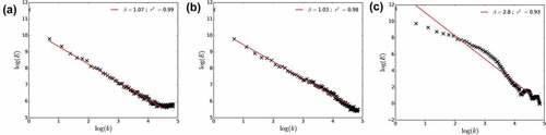
The spectra (Equation 4) obtained with the three approaches are displayed in Fig. 7. One thousand samples of size 256 simulated with $\alpha =1.6$, $C_1=0.2$ and $h=1$ are used as input into the analysis. With the first approach, there is a flattening of the spectra for small scales (Fig. 7(a)). The scaling behaviour is strongly altered with the third approach (Fig. 7(c)), while it is very good with the second one (Fig. 7(b)). Hence, it was decided to keep this second approach in the following. One could argue that since $S_n^1\left(\alpha ,h\right)$ does not reach its final value $S^1\left(\alpha ,h\right)$ before 4–5 steps, we should perform 4 or 5 additional cascade steps and then average back to the desired resolution. This would result in too great a computation time, especially in 2D. Since the scaling behaviour was found to be very good with only two additional steps, it was chosen not to perform more. Similar results are found with other values of $\alpha$, $C_1$ and h.

Figure 7. Spectral analysis of the field generated with the three approaches tested to finish the blunt discrete cascade process. Simulations with $\alpha =1.6$, $C_1=0.2$ and $h=1$ are used.

Finally, the whole process of blunt discrete UM cascades is summarized in Fig. 8.

Figure 8. Schematic description of the generation of a blunt multiplicative cascade process A from a standard one B.

3.5 Extension to 2D fields

The blunt cascade process was introduced in 1D (for time series) and its extension is rather straightforward in 2D (for maps). The process in 2D is obtained by simply implementing the moving window successively on each line and then rows of the 2D field. In a similar way as in 1D, we find a $S^2\left(\alpha ,h\right)$ which is the equivalent of $S^1\left(\alpha ,h\right)$ and it also corresponds to an asymptotic limit reached after a few cascade steps as displayed in Fig. 6(a). This value should be used in the renormalization of the a’. $S^2\left(\alpha ,h\right)$ is simply $S^1\left(\alpha ,h\right)$ raised to the power 2, which is why this notation was chosen:

(21) $S^2\left(\alpha ,h\right)={\left[S^1\left(\alpha ,h\right)\right]}^2$(21)

Same patterns as in 1D for the dependence of $S^2\left(\alpha ,h\right)$ with regards to $\alpha$ and h are found and shown in Fig. 6(b) and (c).

4 Results

4.1 Examples of simulations

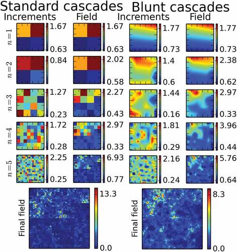
Figures 9 and 10 display the generation process in 1D and 2D, respectively, for simulations with $\alpha =1.6$, $C_1=0.2$ and $h=1$. The final length of the time series in 1D is 256 time steps and the final size of the map in 2D is 64 × 64. Note that in 1D the full increment fields are shown and not only the middle portion as in 2D, which is actually the one used in the field generation because of the side effects previously mentioned. The progressive, cascade step by cascade step, addition of variability to the field is visible and highlights the whole interest of cascade processes. The effect of the blunting is also visible, notably in 2D. Indeed, the sharp unrealistic structures of the standard field are replaced by blunted ones. With greater values of h, the smoothing of the increment fields would even be more pronounced.

Figure 9. Illustration in 1D of the simulation of a field with the help of a standard cascade process B and the corresponding blunt one A. The first five cascade steps are shown, as well as the final fields of length 256 time steps. Values of $\alpha =1.6$, $C_1=0.2$ and $h=1$ are used.

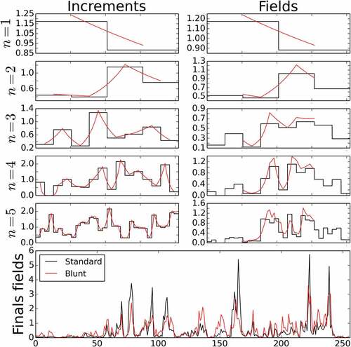
Figure 10. Illustration in 2D of the simulation of a field with the help of a standard cascade process B and the corresponding blunt one A. The first five cascade steps are shown, as well as the final fields of size 64 × 64 pixels. Values of $\alpha =1.6$, $C_1=0.2$ and $h=1$ are used.

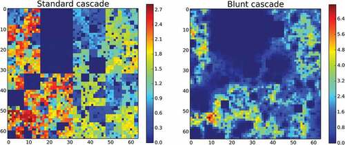
Finally, let us mention an issue that is found with small values of $\alpha$. Figure 11 shows the fields obtained with the standard process and the corresponding blunt one with $h=1$. With such parameters, some extremely small values of increments are generated (in dark blue on the right panel). They are so small that when used in a geometric average, they make the outcome close to zero as well. This results in increasing the size their influence. Such effect explains the dark blue boxes on the field obtained with the blunt cascades (left panel). This is actually a visual characterization of the fact that for $\alpha <1$ the $C_1$ is increased by the blunting ($S^d\left(\alpha ,h\right)$>1). This effect is more pronounced with increasing values of h. Such square structures found for small values of $\alpha$ are a limitation of the innovative blunt process, which means it should preferably be used for field with $\alpha >1$ as is the case for rainfall.

Figure 11. Example of output in 2D of simulations with $\alpha =1.6$, $C_1=0.1$ and $h=1$.

4.2 Back to the stationarity

One of the goals of the singularities’ blunting introduced in this paper was to address the fact that the stationarity features are poorly represented in fields simulated with the standard cascade process B. Hence, as it was done for this process, the quantity $⟨A_j^q{A}_{j+t}^q⟩$ obtained with series of size 256 was studied for various t and j. The same curves as the ones that were studied for B in Fig. 2(a) are plotted in Fig. 2(b) for a blunt process A with $h=1$. The asymmetry was removed as required. The curves for various j are not exactly equal. The reason behind the small remaining differences can be understood from Equation (16). Indeed, despite the fact that the ‘powers of increment shared’ between two time steps do not depend on their position within the series but only on the lag between them (discussion in Section 3.2), their precise distribution according to increments within each cascade level differs. As a consequence, when correlations are studied, the averages will be slightly different. Nevertheless, the stationarity of the blunt cascade process has been strongly improved with regards to the standard process. As it was expected, similar results are obtained when increasing the values of h with stronger correlations. This is illustrated in Fig. 2(c), which displays the same curves but for $h=4$.

4.3 Multifractal analysis of simulated fields

In this section, we test the validity of Equation (20), which relates UM parameters input in the simulations to the expected ones in the blunt cascade process. The results are first discussed for $h=1$. Other values of $h$ are addressed at the end of this section. The 1D case, i.e. time series, is discussed first. All the possible combinations of UM parameters for $\alpha \subset \left[0.2,0.4,0.6,1,1.2,1.4,1.6,1.8\right]$ and $C_1\subset \left[0.1,0.2,0.3,0.4,0.5\right]$ are tested. For each of the 40 sets of UM parameters, a full UM analysis is carried out on 1000 realizations of length 256. Figure 12 displays the outcome of such an analysis for $\alpha =1.6$, $C_1=0.2$ and $h=1$. It appears that the scaling behaviour is excellent, with coefficients of determination $r^2$ of the linear regression in the trace moment analysis all greater than 0.99 (Fig. 12(a)). This confirms the outcome of the spectral analysis, which was already displayed in Fig. 7(b). The DTM curves used for the determination of $\alpha$ and $C_1$ (Fig. 12(b)) also exhibit the expected shape, enabling a robust estimation of the parameters. For this example, we find $\alpha =1.62$ and $C_1=0.14$. Such consistent scaling behaviour is retrieved for all other sets of UM parameters with $r^2$ always greater than 0.99. It should be mentioned the same excellent scaling behaviour was also found in the simulations with the standard cascade process.

Figure 12. Multifractal analysis of 1000 realizations of the blunt cascade process A for $\alpha =1.6$, $C_1=0.2$ and $h=1$. (a) Trace moment analysis (Equation (1)) and (b) double trace moment analysis.

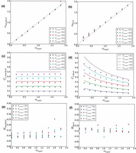
The UM parameters estimated on numerical simulations are compared with the ones input in the simulations in Fig. 13 for both a standard UM discrete cascade process (left column) and a blunt UM discrete cascade process (right column). In the first row, $\alpha$ for the simulations vs. ${\alpha }_{\mathrm{i}\mathrm{n}\mathrm{p}\mathrm{u}\mathrm{t}}$ is plotted. For the standard cascade process, all the points are along the bisector as expected. For the blunt cascade, the expected behaviour is retrieved for $\alpha >1$ and there is a slight overestimation for smaller values. $C_1$ is plotted against ${\alpha }_{\mathrm{i}\mathrm{n}\mathrm{p}\mathrm{u}\mathrm{t}}$ on the second row with points for the empirical estimations, and a solid line for the expected behaviour according to Equation (20). For great values of $\alpha$ (>1) and small values of $C_1$ (<0.3–0.4), the expected behaviour is observed, which confirms the validity of the calculations that led to Equation (20). For smaller values of $\alpha$ and greater values of $C_1$, some discrepancies appear. The overestimation of $C_1$ is related to the ‘spread’ of the very small values in the geometric interpolation that was previously discussed and generates greater values of $C_1$. It should be noted that a shift is also observed for great values of $C_1$ with the standard cascades (Fig. 13(c)). With regard to H, the re-normalization of the increments $a_{n,j}$ enables us to basically keep the same small values of H, with only a slight increase of roughly 0.05 being noted.

Figure 13. Comparison for time series (1000 1D realizations of length 256) of UM parameters estimated on numerical simulations for both standard UM discrete cascade process (left) and blunt UM discrete cascade process with $h=1$ (right) with regard to parameters input to the simulations.

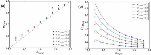
The same analyses were carried out in 2D, except with 100 samples and not 1000 samples to limit computation time. The sample size is 64 × 64. Figure 14 displays the main comparison plots. Only the plots with the UM parameters for the blunt process (again with $h=1$) are shown, the others are similar to the ones obtained in 1D. The relation for $\alpha$ remains true for $\alpha >1$ and $C_1$ <0.3–04. With regard to $C_1$, the same discrepancies as in the 1D case are noted, but in a less pronounced way.

Figure 14. As in Fig. 13, comparison for maps (100 2D realizations of size 64 × 64) of UM parameters estimated on numerical simulations for blunt UM discrete cascade process with regard to parameters input to the simulation. A value of $h=1$ was used.

Finally, the outcome of the analysis when considering h > 1 should be discussed. The main results in 1D are shown in Fig. 15, which displays an indication of the scaling ($r^2$ in the TM analysis for $q=1.5$), and the UM parameters $\alpha$, $C_1$ and H, all as a function of h for simulations with $\alpha =1.6$ and $C_1=0.2$ as inputs. As before, 1000 series of length 256 are used. To limit the influence of the edge effects getting worse with increasing values of h, series of length 1024 were simulated and only a 256 portion in the middle analysed. First, it appears that the quality of the scaling slightly decreases with increasing values of h (Fig. 15(a)). This is actually not surprising since increasing values of h yield also greater values of H (Fig. 15(b)), and that the TM analysis which is used here assumes that the studied field is conservative. This is no longer the case when large values of h are used. With regard to $C_1$ (Fig. 15(d)), the estimated value on the simulations decreases with h and behaves as expected according to Equation (20); $\alpha$ remains constant as expected as well.

Figure 15. Plots of the UM parameters $\alpha$, $C_1$ and H along with an indication of the scaling quality ($r^2$ of the linear regression in the TM analysis for $q=1.5$), as a function of h input in the numerical simulations. Values of $\alpha =1.6$ and $C_1=0.2$ are used as inputs in the simulations. One thousand 1D realizations of size 256 are used.

In summary, the analysis carried out on numerical simulations illustrated by Figs. 13–15 shows that the theoretical expectations of Equation (20) are retrieved over the range of UM parameters $\alpha >1$, $C_1$<0.3–04 for $h<7$, which are the ones most relevant for rainfall.

Before continuing, let us say a few words about the issue of zeros in the simulated fields and their relation to the topic of the intermittency of rainfall process, understood here as the study of the alternation of dry and rainy time steps/areas. Zeros is indeed a key feature of rainfall that is not directly simulated with the model introduced here, which will only be able to simulate (potential extremely) small values. By interpolating the increments at each resolution, it will tend to decrease the intermittency. Nevertheless, since it is a geometric interpolation that is carried out, the near-zero values will have a tendency to spread. In order to check this issue, simulated series have been normalized and ‘thresholded’ (i.e. all values smaller than 0.3 are artificially set to zero) in order to mimic the limit of detection of any measuring device. For simulations with $\alpha =1.6$ and $C_1=0.2$, a fractal dimension of 0.85 is found for $h=0$ and of 0.88 for $h=1$. This suggests that the blunting of the increments tends to reduce the simulated intermittency. Anyway, the issue of the simulation of the zeros in rainfall fields remains an open question (see Gires et al. 2013). Further developments of this model will be needed to properly account for them. As a consequence, only applications focusing on rainfall events will be considered in this paper, since during such a period, the issue of the zeros has much less influence.

5 Application of blunt cascades for downscaling rainfall fields

5.1 Overall concepts

The aim of this section is to present how blunt discrete cascades can easily be used to address downscaling, which is a very common issue encountered with geophysical fields. Downscaling has often been addressed with the help of multifractal cascades (Deidda 2000, Olsson et al. 2001, Biaou et al. 2003, Ferraris 2003, Rebora et al. 2006, Gires et al. 2014b). In this paper, we suggest to use blunt cascades to keep using the convenient discrete cascades while removing the sharp unrealistic transitions in simulated fields.

The basic assumption underlying the presented applications is that the studied fields are generated with the help of blunt discrete cascade process of known UM parameters $\alpha$ and $C_1$. This assumption can actually be checked on the available data through a multifractal analysis, which also enables us to estimate the characteristic parameters. The methodology for downscaling is rather straightforward in the convenient framework of discrete cascades, which are intrinsically a downscaling model, and it simply consists in generating the additional steps to increase the resolution. Basically, all the missing underlying increments of the standard process (the $b_{n,i}$ using the notation of this paper) are stochastically generated. 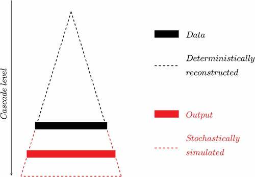From them, the $a_{n,j}$ and ultimately the field is derived. This is summarized in Fig. 16 and consists, more precisely, in four steps:

Figure 16. Schematic presentation in 1D of the downscaling procedure that is implemented in this paper.

Step 1. Estimation of the UM parameters. This is done by performing a multifractal analysis of the available data. Such estimation is done at coarse resolution, and it is assumed that they remain valid for higher resolutions (or smaller scales), i.e. that there is no scaling break. It should be noted that following Equation 20, the parameters actually input in the simulation will be $\alpha$ and $C_1/S^d\left(\alpha ,h\right)$ to retrieve the correct one $\alpha$ and $C_1$ once the blunting has been implemented.

Step 2. Estimating the starting point of the cascade process. The only tricky point in the process is to compute the product of the blunt increments $a_{n,j}$ for the ‘known’ portion of the cascade. This corresponds to the outcome of the cascade process at the initial resolution (the black rectangle in Fig. 16). This corresponds to ‘inserting’ the available data in the cascade process. This is done by performing a linear interpolation of the initial low-resolution field at the maximum resolution used in the cascade process. In practice, it is a ‘blunting’ of the data with $h=1$. By the way, this can be considered as a simplistic way of downscaling a field.

Step 3. Stochastically simulating the missing increments. The missing increments at the higher resolutions (in red on Fig. 16) are stochastically drawn. It should be noted that two steps more than needed with regard to the desired final resolution are implemented.

Step 4. Generating the fields at the desired resolution. The increments at the higher resolutions are then blunt and multiplied to the initial data at low resolution (point (2)). It is the same process as in the simulation of a field (Section 4.1) except that, instead of using the blunt increments for the coarse resolution, the initial data is used.

The fact that the missing unknown increments are stochastically generated in the downscaling process means that not only a single deterministic result but an ensemble of realistic realizations will be obtained. More precisely, the outcome of the process is not a deterministic value but an empirical probability distribution. In order to quantify the variability within the simulated ensemble of high-resolution fields, quantiles (10%, 50% and 90%) are computed.

In Sections 5.2 and 5.3, this methodology is implemented in 1D and 2D, respectively, which enables us to both highlight its advantages and discuss its current limitations to establish a road map for future developments. In 2D, the results are compared with the ones that would be obtained with standard discrete cascades for illustrative purposes. In general, no comparison is carried out with the other techniques available in the literature. This would be beyond the scope of this paper, which is about presenting an innovative blunt discrete cascade process and proof of concepts through downscaling applications. Proper comparison with other methodologies should definitely be carried out in future investigations.

5.2 Implementation in 1D

5.2.1 Data

An OTT Parsivel¹ disdrometer (Battaglia et al. 2010; OTT, 2014) located on the roof of the Carnot building of the Ecole des Ponts ParisTech campus near Paris, was used to collect the rainfall data manipulated in this sub-section. This device is actually part of the TARANIS observatory of the Fresnel Platform of École des Ponts ParisTech.² Interested readers are referred to Gires et al. (2018) for more details on the device functioning and measurement campaigns. The climate of the area is temperate, with a mean annual rainfall of roughly 640 mm² rather homogeneously distributed throughout the year. In this paper, the data collected between 15 January 2018 and 9 December 2018 is used with 1-min time steps. More precisely, 61 rainy periods of duration 256 min are extracted corresponding to a total rainfall amount of 229 mm.

A multifractal analysis was carried out on average on these series and the scaling behaviour is found to be excellent (with TM analysis $r^2>0.99$) with $\alpha =1.92$, $C_1=0.13$ and $H=0.36$. Such values are usual for rainfall fields during a rainfall event. This analysis was carried out on the fluctuations of the field, as recommended in Lavallée et al. (1993).

5.2.2 Results and discussion

The output of the downscaling process in 1D is shown in Fig. 17. First, illustrations with a 256-min rainfall period that occurred on 29 April 2018 are displayed on the upper line for a downscaling from 8 min to 1 min (Fig. 17(a)) and from 64 min to 1 min (Fig.17(b)). The data is first aggregated to 8 min (or 64 min) which corresponds to the step functions in dash blue in the figures. This raw initial data is then interpolated at the highest resolution (using the same process as for the blunting with $h=1$). It is this series (solid blue) that are then used as a starting point in the downscaling process. UM parameters of this specific series ($\alpha =1.77$, $C_1=0.14$) are used and $h=6$.

Figure 17. Downscaling in 1D. (a) Output of the downscaling process from 8-min time steps to 1-min time steps for a 256-min rainfall period that occurred on 29 April 2018. One thousand realizations of the downscaled series are generated and the light red area corresponds to the 5–95% quantile interval. (b) As for (a), but for a downscaling from 64 min to 1 min. (c) Distribution of values according to bins of singularities γ for the downscaling process from 8-min time steps to 1-min steps. (d) As in (c), but for the downscaling process from 8-min time steps to 1-min steps.

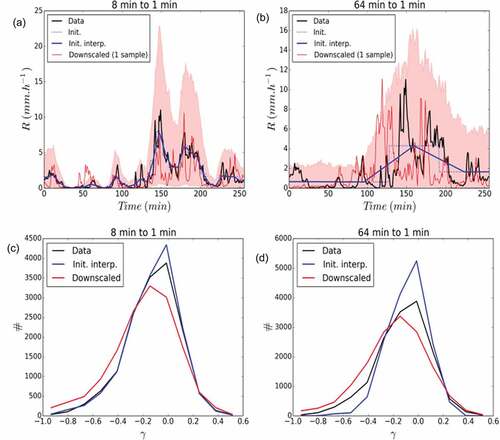
One thousand realizations of the downscaled field are then generated. The light red shadow area corresponds to the 5–95% quantile interval computed for each time step. A single realization of downscaled fields is plotted in solid red. In both cases, the actual data is located within the expectations and each individual realization exhibit visually a behaviour that is similar to the observed series.

Such visual interpretation is confirmed through a more quantitative analysis, in which all the 61 rainfall periods studied in this paper are first up-scaled (to 8 min or 64 min) and then downscaled, using for each of their own UM parameters $\alpha$ and $C_1$ and the same $h=6$.

First, a multifractal analysis of the obtained downscaled series was carried out and showed that the downscaled series exhibited excellent scaling behaviour furthermore very similar to the one of the measured data at the highest resolution, which was a requirement. For instance, for the downscaling from 8 min to 1 min, we find $r^2$ equal to 0.99 (for $q=1.5$ in the TM analysis), $\alpha =1.81$, $C_1=0.17$, and $H=0.32$. For the downscaling from 64 min to 1 min, we find $r^2$ equal to 0.99 as well and $\alpha =1.94$, $C_1=0.16$, and $H=0.32$. Similar values are found for other realizations of the whole downscaling process. Then, the distribution of the observed values is studied by counting the number of value found within singularity bins. The singularity $\gamma$ is obtained from the rain rate by using the relation $R={\lambda }^{\gamma }$. Twenty bins are used, and the obtained distribution is displayed in Fig. 17(c) (downscaling from 8 min to 1 min) and Fig. 17(d) (downscaling from 8 min to 1 min). The downscaling process enables to retrieve properly the observed distribution, notably for the greatest singularities. This means the ‘blunt’ cascade process enables to properly reproduce the extremes. It should nevertheless be mentioned that there is slight over-representation of the small singularities and under-representation of middle singularities in the downscaling process.

The distribution of the initial data (interpolation of the up-scaled observed data at 8 min and 64 min) was plotted for illustrative purposes to highlight the need not to limit the analysis to the distribution of values of the final field. Indeed, despite an obvious large under-representation of the number of great singularities, and over-representation of middle singularities, they overall look correct. But the scaling behaviour for these fields is very poor meaning they are not realistic. For example, for 64 to 1 min case, $r^2$ found is equal to 0.72, and $\alpha =0.45$, $C_1=0.08$, which is very far from the estimates retrieved on the actual data.

As long as there is no scaling break, downscaling between other resolutions, i.e. for example from daily to hourly rainfall, could be implemented with this methodology. If the scaling behaviour exhibits a break, then various sets of UM parameters should be used according to the cascade level.

5.3 Implementation in 2D

5.3.1 Data

Rainfall maps used in this paper were obtained from a X-band radar operated by Ecole des Ponts ParisTech on its campus (see Paz et al. 2018 for more details on the device and hydrological applications). The resolution of the data provided by the radar is 250 m × 250 m. Two time steps (08:32 and 09:06 UTC) corresponding to the accumulation over 3 min and 40 s of an event that occurred on 16 September 2015 are used. They were chosen because they exhibit different visual patterns.

A portion of 128 × 128 pixels is selected for the analysis. This radar data is shown in Fig. 18(a) for the first time step (08:32 UTC) and in Fig. 19(a) for the second one (09:06 UTC). A good scaling behaviour on the range of scales [250 m to 2 km] was found for both time steps. Multifractal analysis yields $\alpha =1.65$, $C_1=0.072$ and $H=0.43$ for the first time step (08:32 UTC). 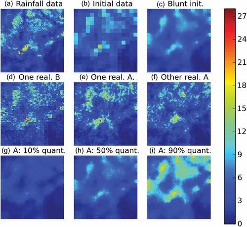$\alpha =2.0$, $C_1=0.033$ and $H=0.34$ are retrieved for the second time step (09:06 UTC).

Figure 18. Illustration of the downscaling process for the time step 2015-09-16 08:32 (UTC). Unit is mm h⁻¹.

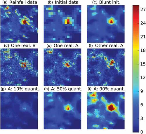
Figure 19. Illustration of the downscaling process for the time step 2015-09-16 09:06 (UTC). Unit is mm h⁻¹.

Before implementing the downscaling process, the data resolution is degraded to pixels of size 2 km × 2 km by simply averaging over adjacent 8 × 8 pixels. This low-resolution field is used as initial data and denoted this way. This is displayed in Figs. 18(b) and 19(b). The downscaling process is used to generate fields at the resolution of 250 m × 250 m; i.e. three disaggregation steps are needed to decrease by a ratio of 8 the pixel size (note that in practice two more steps will be implemented for the practical reasons previously mentioned). The initial data interpolated at the highest resolution is displayed in panel Figs. 18(c) and 19(c) for each time steps.

5.3.2 Results and discussion

Let us first discuss the results obtained on the 08:32 UTC time step (Fig. 18). Figure 18(d) displays a realization of downscaled field obtained with the help of a standard B process. The unrealistic sharp squares are visible and too great values are also obtained with regards to the original radar data. Figure 18(e,f) displays two different realizations for the blunt process A with $h=6$. As expected, the square structures have been removed, and the visual aspects of these simulated downscaled fields are much more satisfactory. In addition, the small-scale values within heavy areas which are visible in the standard case are mostly removed in the blunt case. Quantitatively, as in 1D, the expected multifractal behaviour is retrieved. One can note that, for the realization in Fig. 18(e), the rainy area in the northwest is well represented, while it is not in the realization of Fig. 18(f). Both realizations simulate a ‘potential’ version of heavy rainfall area in the middle.

Figure 18(g), (h) and (i) displays, respectively, the 10%, 50% and 90% quantile obtained for each pixel with the help of 100 realizations of downscaled blunt rainfall fields. As expected, the 50% quantile map yields a map very similar to the initial data put at the maximum resolution (Fig. 18(c)), while the other two maps provide a quantification of the uncertainty associated with the downscaling process. It should be mentioned that, in this case, the heavy spot in the south is underestimated with the blunt process. The small square structures visible on the sides (notably on Fig. 18(i)) are simply due to the fact that the increments that would be needed to implement the blunting of the side increments are not simulated. This could be solved very easily in practice by simulating a larger area and only taking the middle portion. This was not done here for computational time reasons.

Figure 19 shows the same information as Fig. 18, but for the other time step (09:06 UTC). Given that the estimated value of H was lower for this time step, a value of h equal to 4 was used instead of h = 6 in the previous simulations. The outcome basically confirms the comments made on the previous time step. Its addition, Fig. 19(e,f) illustrates that the blunt process is notably able to generate field with a realistic aspect for intermediate intensities.

6 Conclusion

In this paper, we introduced a novel approach to lessen one of the main limitations of the discrete random multiplicative cascades, which is their lack of stationarity. The developed process basically consists in interpolating at each cascade steps the random multiplicative increments at a higher resolution than the desired final one. The interpolation is performed geometrically on the multiplicative increments or equivalently linearly on their corresponding singularity. It is established theoretically, and numerically confirmed, that the simulated fields would also exhibit a multifractal behaviour with an unchanged multifractality index $\alpha$ and with a mean intermittency codimension $C_1$ changed to $C_1{S}^d\left(\alpha ,h\right)$. $S^d\left(\alpha ,h\right)$can easily be computed and depends on $\alpha$, the embedding dimension d of the field, and a parameter h corresponding to the number of multiplicative increments at a given cascade level that are influencing the blunt ones. It is shown that such an approach remains only valid over a limited range of UM parameters due to strong deviations noted for small $\alpha$ (<1) and large $C_1$ (>0.3–0.4). This limits the potential applications.

The methodology to use blunt discrete cascade processes to address downscaling is presented. It is then applied in 1D with disdrometer data and in 2D with radar data coming from the Paris area. This enables to confirm the validity of the suggested process and discuss the current limitations. Given that the model was shown to behave well over a given range of UM parameters, it should be able to adapt to other types of climate. Further investigations with other types of climate would be needed to confirm this.

This newly developed process opens the path for future developments both theoretical and practical:

1. to improve how the zeros of the rainfall fields are added (see Gires et al. 2013, for a complete discussion on the topic);

2. to extend it to the space–time process. Following the approach of Biaou et al. (2003) tested in Gires et al. (2014a; 2014b), who introduced a simple anisotropy exponent between space and time, it seems feasible apart from computational limitations that will have to be addressed;

3. to introduce advection and spatial anisotropy in the simulated fields notably to enable nowcasting applications, for which the approach developed by Seed (2003) and Niemi et al. (2014) could be helpful.

Disclosure statement

No potential conflict of interest was reported by the authors.

Additional information

Funding

The authors gratefully acknowledge partial financial support from the Chair “Hydrology for Resilient Cities” (endowed by Veolia) of Ecole des Ponts ParisTech, and the Île-de-France region RadX@IdF Project.

Notes

¹ Source http://www.meteofrance.com/climat.

² https://hmco.enpc.fr/portfolio-archive/fresnel-platform/.

References

- Battaglia, A., et al., 2010. PARSIVEL snow observations: a critical assessment. Journal of Atmospheric and Oceanic Technology, 27 (2), 333–344. doi:10.1175/2009JTECHA1332.1.
- Biaou, A., et al., 2003. Fractals, multifractals et prévision des précipitations. Sud Sciences Et Technologies, 10, 10–15.
- Chambers, J.M., Mallows, C.L., and Stuck, B.W., 1976. Method for simulating stable random-variables. Journal of the American Statistical Association, 71, 340–344. doi:10.1080/01621459.1976.10480344
- Deidda, R., 2000. Rainfall downscaling in a space-time multifractal framework. Water Resources Research, 36, 1779–1794. doi:10.1029/2000WR900038
- Ferraris, L., 2003. A comparison of stochastic models for spatial rainfall downscaling. Water Resources Research, 39 (12). doi:10.1029/2003WR002504
- Gaume, E., Mouhous, N., and Andrieu, H., 2007. Rainfall stochastic disaggregation models: calibration and validation of a multiplicative cascade model. Advances in Water Resources, 30 (5), 1301–1319. doi:10.1016/j.advwatres.2006.11.007.
- Gires, A., et al., 2013. Development and analysis of a simple model to represent the zero rainfall in a universal multifractal framework. Nonlinear Processes in Geophysics, 20 (3), 343–356. doi:10.5194/npg-20-343-2013.
- Gires, A., et al., 2014a. Impacts of small scale rainfall variability in urban areas: a case study with 1d and 1d/2d hydrological models in a multifractal framework. Urban Water Journal. doi:10.1080/1573062X.2014.923917.
- Gires, A., et al., 2014b. Influence of small scale rainfall variability on standard comparison tools between radar and rain gauge data. Atmospheric Research, 138, 125–138. doi:10.1016/j.atmosres.2013.11.008
- Gires, A., Tchiguirinskaia, I., and Schertzer, D., 2018. Two months of disdrometer data in the Paris area. Earth System Science Data, 10 (2), 941–950. doi:10.5194/essd-10-941-2018.
- Gupta, V.K. and Waymire, E., 1993. A statistical analysis of mesoscale rainfall as a random cascade. Journal of Applied Meteorology, 32, 251–267. doi:10.1175/1520-0450(1993)032<0251:ASAOMR>2.0.CO;2
- Hubert, P., 2001. Multifractals as a tool to overcome scale problems in hydrology. Hydrological Sciences Journal, 46 (6), 897–905. doi:10.1080/02626660109492884
- Kolmogorov, A.N., 1941. Local structure of turbulence in an incompressible liquid for very large Reynolds numbers. Proceedings of the USSR Academy of Sciences, 30, 299.
- Lavallée, D., Lovejoy, S., and Ladoy, P., 1993. Nonlinear variability and landscape topography: analysis and simulation. In: L. de Cola and N. Lam, eds. Fractals in geography. Englewood Cliffs, NJ: Prentice-Hall, 171–205.
- Licznar, P., Lomotowski, J., and Rupp, D.E., 2011. Random cascade driven rainfall disaggregation for urban hydrology: an evaluation of six models and a new generator. Atmospheric Research, 99 (3–4), 563–578. doi:10.1016/j.atmosres.2010.12.014
- Lovejoy, S. and Schertzer, D., 2010a. On the simulation of continuous in scale universal multifractals, part I spatially continuous processes. Computers & Geosciences, 36 (11), 1393–1403. doi:10.1016/j.cageo.2010.04.010
- Lovejoy, S. and Schertzer, D., 2010b. On the simulation of continuous in scale universal multifractals, Part II space-time processes and finite size corrections. Computers & Geosciences, 36 (11), 1404–1413. doi:10.1016/j.cageo.2010.07.001
- Menabde, M. and Sivapalan, M., 2000. Modeling of rainfall time series and extremes using bounded random cascades and Levy-stable distributions. Water Resources Research, 36 (11), 3293–3300. doi:10.1029/2000WR900197
- Müller, H. and Haberlandt, U., 2018. Temporal rainfall disaggregation using a multiplicative cascade model for spatial application in urban hydrology. Journal of Hydrology, 556, 847–864. doi:10.1016/j.jhydrol.2016.01.031
- Niemi, T.J., Kokkonen, T., and Seed, A., 2014. A simple and effective method for quantifying spatial anisotropy of time series of precipitation. Water Resources Research, 50 (7), 5906–5925. doi:10.1002/2013WR015190
- Olsson., J., 1998. Evaluation of a scaling cascade model for temporal rainfall disaggregation. Hydrology and Earth System Sciences, 2 (1), 1930. doi:10.5194/hess-2-19-1998
- Olsson, J., Uvo, C.B., and Jinno, K., 2001. Statistical atmospheric downscaling of short-term extreme rainfall by neural networks. Physics and Chemistry of the Earth Part B-Hydrology Oceans and Atmosphere, 26 (9), 695–700. doi:10.1016/S1464-1909(01)00071-5
- OTT, 2014. Operating instructions, present weather sensor ott parsivel2. Kempten, Germany: OTT.
- Over, T.M. and Gupta, V.K., 1996. A space-time theory of mesoscale rainfall using random cascades. Journal of Geophysical Research-Atmospheres, 101 (D21), 26319–26331. doi:10.1029/96JD02033
- Paz, I., et al., 2018. Multifractal comparison of reflectivity and polarimetric rainfall data from c- and x-band radars and respective hydrological responses of a complex catchment model. Water (Switzerland), 10 (3). doi:10.3390/w10030269.
- Rebora, N., et al., 2006. RainFARM: rainfall downscaling by a ltered autoregressive model. Journal of Hydrometeorology, 7 (4), 724–738. doi:10.1175/JHM517.1
- Rupp, D.E., et al., 2012. Multiplicative cascade models for ne spatial downscaling of rainfall: parameterization with rain gauge data. Hydrology Earth System Sciences, 16 (3), 671–684. doi:10.5194/hess-16-671-2012
- Schertzer, D. and Tchiguirinskaia, I., 2018. Pandora box of multifractals: barely open? In: A. Tsonis, ed. Advances in nonlinear geosciences. Cham: Springer, 543–563.
- Schertzer, D. and Lovejoy, S., 1987. Physical modelling and analysis of rain and clouds by anisotropic scaling and multiplicative processes. Journal of Geophysical Research, 92 (D8), 9693–9714. doi:10.1029/JD092iD08p09693
- Schertzer, D. and Lovejoy, S., 1997. Universal multifractals do exist!: comments. Journal of Applied Meteorology, 36 (9), 1296–1303. doi:10.1175/1520-0450(1997)036<1296:UMDECO>2.0.CO;2
- Seed, A.W., 2003. A dynamic and spatial scaling approach to advection forecasting. Journal of Applied Meteorology, 42 (3), 381–388. doi:10.1175/1520-0450(2003)042<0381:ADASSA>2.0.CO;2