Monthly suspended sediment load prediction using artificial intelligence: testing of a new random subspace method

ABSTRACT

The predictive capability of a new artificial intelligence method, random subspace (RS), for the prediction of suspended sediment load in rivers was compared with commonly used methods: random forest (RF) and two support vector machine (SVM) models using a radial basis function kernel (SVM-RBF) and a normalized polynomial kernel (SVM-NPK). Using river discharge, rainfall and river stage data from the Haraz River, Iran, the results revealed: (a) the RS model provided a superior predictive accuracy (NSE = 0.83) to SVM-RBF (NSE = 0.80), SVM-NPK (NSE = 0.78) and RF (NSE = 0.68), corresponding to very good, good, satisfactory and unsatisfactory accuracies in load prediction; (b) the RBF kernel outperformed the NPK kernel; (c) the predictive capability was most sensitive to gamma and epsilon in SVM models, maximum depth of a tree and the number of features in RF models, classifier type, number of trees and subspace size in RS models; and (d) suspended sediment loads were most closely correlated with river discharge (PCC = 0.76). Overall, the results show that RS models have great potential in data poor watersheds, such as that studied here, to produce strong predictions of suspended load based on monthly records of river discharge, rainfall depth and river stage alone.

KEYWORDS:

• suspended sediment
• rivers
• artificial intelligence
• random forest
• random subspace
• support vector machine

Editor S. Archfield Associate editor P. Srivastava

1 Introduction

The prediction of suspended sediment load in rivers is one of the most important issues in the field of water resources management and river engineering (Melesse et al. 2011, Kisi et al. 2012, Lafdani et al. 2013). Suspended sediment can directly affect the capacity of reservoir storage, operation of hydraulic structures, water quality and dispersion of non-point source pollutants (Melesse et al. 2011, Fan et al. 2012, Tang et al. 2014). The Suspended sediment load is the result of several physical processes including detachment, transportation and deposition of grains, which depends on the magnitude and intensity of precipitation, discharge in the river network, physical characteristics of the soil, topography and land use. In many studies, rainfall and discharge are reported as the most important controlling factors for suspended sediment load (Jie and Yu 2011). However, human activity such as land-use change, and in particular deforestation, can increase fine sediment input to rivers (Ali and Abbas 2013, Heng and Suetsugi 2014, Bathrellos et al. 2017). In this sense, suspended sediment load in rivers can be considered as the cumulative result of watershed management practices (Cigizoglu 2004).

The impact of poor land management practices are clearly seen in rivers in Iran. These rivers carry much higher suspended sediment loads than similar rivers in neighboring countries. For example, Aras, Haraz and Sefid-roud rivers in Iran carry around 8, 7.5 and 8.9 g/l but Euphrates (Al-Furat) in Syria, Tigris in Iraq and Kabul in Afghanistan carry about 0.1, 1.2 and 1.1 g/l, respectively (Ahmadi 2010). Therefore, accurate estimation of the temporal variation in suspended sediment load in Iranian rivers is paramount to assess current watershed management practices and their future optimization.

Like many other processes in rivers, suspended sediment dynamics are complex and non-linear (Nourani 2009, Rajaee 2011) due to hysteresis effects (Mao and Carrillo 2017). As a result, modelling suspended sediment dynamics requires a robust and reliable model with a non-linear structure (Dai and Lu 2010, Kisi et al. 2012, Wenske et al. 2012, Vigiak et al. 2017). Some methods, such as process-based models, empirical relationships and statistically-based models (Melesse et al. 2011) have been developed to predict suspended sediment load and its relationship with driving variables such as rainfall and river hydraulics (e.g. velocity, discharge and shear stress). Process-based models usually require many variables and detailed spatial and temporal environmental data for the model build, calibration and validation (Kisi et al. 2012, Hamel et al. 2017). Such information is rarely available in developing countries, such as Iran, because direct measurement of variables such as river velocity, channel topography, rainfall intensity and suspended sediment is expensive. Furthermore, process-based simulations are complex, time-consuming and require highly-skilled end users that do not always reside in these countries (Jha and Bombardelli 2011).

Recently, development of artificial intelligence has opened up new and exciting ways to predict environmental behavior, including variations in suspended sediment load. Artificial intelligence techniques do not seek to explain the physical processes and mathematical reasoning for changes in environmental behavior but to recognize patterns, both expected and unexpected, within data. These patterns can highlight environmental relationships in space and time that may unveil critical details about behavior, reveal previously unsuspected relationships, or mitigate uncertainty in estimates. Thus these types of techniques are at their most beneficial in situations when process-based models cannot be applied (e.g. lack of understanding of the underlying physics of the process) or that suffer from inadequacies due to the limitation of data. Therefore the key advantage of artificial intelligence methods is that that some parameters which are difficult or expensive to measure, such as suspended sediment load, could be easily predicted using other factors which are more readily available, such as rainfall depth, discharge and river stage. Such attempts have included the use of multi-layer perceptrons (MLPs) (Jain 2001, Cigizoglu 2002, 2004, Kisi 2004, Partal and Cigizoglu 2008), support vector machine (SVM) (Azamathulla and Wu 2011, Lafdani et al. 2013), genetic programing (GP) (Aytek and Kisi 2008, Kisi et al. 2012), and adaptive neuro-fuzzy inference system (ANFIS) (Çimen 2016, Choubin et al. 2018). At present however, there is no consensus over which of these artificial intelligence methods produces the most accurate predictions of suspended sediment load, and more widely, in the prediction of other hydrological parameters.

For example, Melesse et al. (2011) applied four models of MLP – multiple linear regressions (MLR), multiple non-linear regression (MNLR) and autoregressive integrated moving average (ARIMA) – to suspended sediment load prediction in the Mississippi, Missouri and Rio Grande rivers in USA. Their results showed that the MLP models have a higher predictive capability than multiple linear regression, multiple non-linear regression and Autoregressive integrated moving average models. Chiang and Tsai (2011) reported that SVM models outperformed ANN models in estimation of suspended sediment loads in rivers in Taiwan. Zounemat-Kermani et al. (2016) also evaluated the predictive power of SVM and ANN models using different kernel and model algorithms for suspended sediment load estimation in USA and found differing results. They used four different kernels of SVM, namely, linear (SVM-L), polynomial (SVM-P), radial basis function (SVM-RBF) and sigmoid (SVM-S), as well as three ANN model algorithms; the conjugate gradient, gradient descent and Broyden-Fletcher-Goldfarb-Shannon (BFGS) approaches. Their results revealed that the SVM-RBF and ANN-BFGS models outperformed the other models. In a study in China, Li et al. (2016) applied random forest (RF), ANN and SVM methods for prediction of Poyang lake water levels. Their results revealed the RF model produced better predictions of daily water level prediction than the other two approaches. Francke et al. (2008) applied sediment rating curves, ANN, RF, Quantile Regression Forests (QRF) and generalized linear models for estimation of suspended sediment load in Isábena catchment, northeastern Spain. Their results showed that the RF and QRF methods had a better predictive performance than the other methods. In water quality prediction, Shkurin (2015) revealed that the RF model is superior to the SVM and ANN methods. ANN is the most common machine learning method due to computational efficiency but this approach has a black box structure, lower predictive power and higher errors in the modelling phase (Bui et al. 2016). Thus, ANFIS models, which are a combination of ANN and fuzzy logic (FL) models, have been proposed (Khosravi et al. 2018a). ANFIS models generally have a better predictive capability than ANN and FL models, but they are poor at finding the best weight parameters which heavily influences the prediction accuracy (Bui et al. 2016).

In summary, these studies reveal a contrasting set of results over the predictive power of different artificial intelligence methods. Therefore, the main goal of the present study is to explore a range of these methods and to evaluate which provides the most accurate prediction of monthly suspended sediment load, using Haraz River in Iran as a case study. This river is an ideal example to explore because it typically transports a huge volume of suspended load resulting from poor land management practices in the watershed, inappropriate river engineering interventions, and an excess of in-channel sediment mining. We will evaluate three artificial intelligence methods: (1) a new method in the field of hydrology called Random Subspace (RS); (2) SVM with a RBF kernel and a Normalized Polynomial Kernel (NPK); and (3) and RF models that benefit from small error rates and improved noise insensitivity (Mert et al. 2016). The results from the RS model will be compared with those from the SVM and RF techniques whose predictive power has been proven previously (Lafdani et al. 2013, Shkurin 2015). We will also perform a sensitivity analysis for the parameters of the three models. We wish to discover if the new model of RS provides superior predictive power to existing artificial intelligence methods in suspended sediment load prediction, and to evaluate its suitability for use in data scarce regions, such as those of our study watershed.

2 Study area

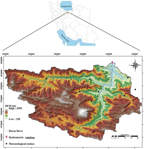
The Haraz watershed is located in the mountainous Mazandaran Province (northern part of Iran) covering an area of about 4014 km², lying between the longitudes of 51°43′ to 52°36′E, and the latitudes of 35°45′ to 36°22′N (Fig. 1). The main causes of flooding, which produces a huge volume of suspended sediment load, are high-intensity, short-duration rainfall events and land-use change (Khosravi et al. 2016). The mean annual rainfall is 723 mm and October is the wettest month of the year with rainfall of 160 mm (Khosravi et al. 2016). The altitude ranges from 300 to 5595 m above sea level and the ground slope varies between 0° and 66°. Geologically, the Haraz watershed is covered by Triassic, Jurassic, Cretaceous, Permian, Tertiary and Quaternary geologic formations. There are four types of soil; in order of prevalence, Inceptisol, Mollisol, Entisol and Alfisol (Choubin et al. 2018). The land use consists of pasture (92%), forest lands (5.9%), barren lands (0.7%), water bodies (0.07%), gardens (0.13%), irrigated land (0.33%) and residential areas (0.24%) (Khosravi et al. 2018c).

Figure 1. Case study location.

3 Data

Monthly river discharge, river suspended sediment discharge, rainfall depth and river stage data from 1972 to 2002 (30 years) from Kareh-Sang Hydrometric Station, which is located at the outlet of the case study, were collected from Mazandaran regional water authority and used in the model building phase, and the data from 2002 to 2010 (8 years) were used for model validation. The rainfall data were collected from various rain-gage stations, from which a spatially-averaged value was derived as model input (Melesse et al. 2011). Table 1 shows the monthly maximum, minimum, mean and standard deviation for stage (S), river discharge (Q), rainfall (R) and suspended sediment discharge (SSL) at Haraz watershed. The mean SSL at the outlet of the Haraz watershed was 2345 ton/day.

Table 1. Statistical summary of the input data. SSD: suspended sediment discharge; SD: standard deviation.

	Stage (m)	Water discharge (m^3/s)	Rainfall (mm)	SSD (t/d)
Maximum	0.225	228.5	176.0	47559
Minimum	0.180	1.3	0.0	44
Mean	0754	30.0	33.1	2345
SD	0.303	22.0	27.5	4799

The distributions of the collected data (Table 2) show that all input variables had positive skewness and positive kurtosis, which shows the possibility of leptokurtic distributions (Melesse et al. 2011). Since the data ($x_i$) do not have a normal distribution, all the input data were normalized ($x_i^{\prime }$) using the following equation to scale the data in the range of 0–1 (Melesse et al. 2011, Lafdani et al. 2013):

(1) $x_i^{\prime }=(x_i-x\mathrm{m}\mathrm{i}\mathrm{n}\mathrm{m}\mathrm{a}{\mathrm{x}}_{\mathrm{m}\mathrm{i}\mathrm{n}.}$(1)

Table 2. Statistical moments of the input data distributions. SSD: suspended sediment discharge.

Moment	Stage	Water discharge	Rainfall	SSD
Skewness	1.4	3.7	1.1	4.9
Kurtosis	3.1	23.5	1.9	32.6

where xmin and xmax refer to the minimum and maximum values of the data, respectively.

4 Machine learning models

4.1 Support vector machine (SVM)

The SVM was first introduced by Vapnik (1995) and Vapnik et al. (1997), and is a supervised learning binary algorithm based on the structural risk minimization and statistical learning method (Bui et al. 2012). The goal of a SVM model is to minimize model complexity and errors. SVM transforms input space into a higher-dimensional feature space to find an optimal separating hyper-plane from a training dataset (Pham et al. 2016). In practice, the SVM can change the nonlinear nature of a variable into a linear one. This technique produces simple and processable classes by construction of a hyper-plane. This mathematical relationship is called a kernel function (Tehrany et al. 2014). An optimal separating hyper-plane is projected in the original space of n coordinates (x_i parameters in vector x) between the points of two distinct classes within a certain error limit (Tehrany et al. 2014). Consider that x and y correspond to input variables and output variables, respectively. If ${\mathrm{x}}_{\mathrm{i}}\in R^n,{\mathrm{y}}_{\mathrm{i}}\in \left\{-1,1\right\}$ and i = 1, …, n, then the optimal separating hyper-plane is calculated using a classification decision function (Tien Bui et al. 2012):

(2) $g\left(x\right)=\mathrm{s}\mathrm{g}\mathrm{n}\left(\sum _{i=1}^n{y}_i{\alpha }_{i}K\left(x_i,x_j\right)+b\right)$(2)

where n is the number of input variables, α_i are Lagrange multipliers, K(x_i, x_j) is the kernel function and b is the offset of the hyper-plane from the origin

The kernel function can be linear, polynomial, RBF or sigmoidal. The two most common kernel functions are the normalized polynomial kernel (NPK) and RBF, although RBF is most often used due to its simple design, good generalization, strong tolerance to input noise, and online learning ability. The NPK and RBF kernel functions are defined, respectively, as follows (Dixon and Candade 2008, Tehrany et al. 2014):

(3) $K\left(x_i,x_j\right)={\left(x_i{x}_j+C\right)}^d$(3)

(4) $K\left(x_i,x_j\right)=\mathrm{e}\mathrm{x}\mathrm{p}{\left(-\gamma x_i-x_j\right)}^2$(4)

where γ controls the degree of nonlinearity of the SVM model and d is the polynomial degree in the kernel function and C is a free parameter trading off the influence of higher-order versus lower-order terms in the polynomial Small and large values of γ cause under- and over-fitting of the training data, respectively. Detailed descriptions of the RF model and their parameters can be found in Lafdani et al. (2013) and Tehrany et al. (2014).

The SVM model was trained using sequential minimal optimization (SMO). SMO is an optimization algorithm used for solving the quadratic programming problem which arises during the training of a SVM model on a dataset. A trial and error method using 10-fold cross-validation techniques was applied to determine the optimal kernel parameters (Pradhan 2013).

4.2 Random forest (RF)

The RF is a flexible, nonparametric, ensemble learning technique first developed by Breiman (2001), and is a hybrid procedure between a decision tree and a regression.RF is composed of multiple trees in which the bootstrap samples are used for constructing each tree (Breiman et al. 1984). The Breiman’s bagging idea and Ho’s (Ho 1995) random selections are the two main processes that constitute the random forest model (Chapi et al. 2017). The RF model assessed the degree to which the estimation error increases when the output of data for certain variables is permuted while all others are left fixed (Pham et al. 2017a). Detailed descriptions of the RF model can be found in Breiman (2001) and Pham et al. (2017a).

During the bootstrap method, the samples which are not included are called out of bag (OOB)These OOB samples from the training set were used to assess the prediction error and thus validate the RF model (i.e. the prediction performance was assessed by evaluating predictions on observations which were not used in the building of the next base learner).

4.3 Random subspace (RS)

The RS model is a classic integrated algorithm that builds a decision tree based on a classifier that supports the highest precision and accuracy for the training data. This method was introduced by Ho (1998) to improve performance of the weak classifiers (Pham et al. 2017b). The RS approach involves randomly drawing samples from the original training set to form a bootstrap sample, which is then used to build the decision tree (Mielniczuk and Teisseyre 2014). For each node of the decision tree, a subset of features are selected randomly, and the best split is chosen. Features in a RS model include attributes, predictors and independent variables. The use of randomly drawn features rather than the entire feature set reduces the correlation between estimators Finally, the tree is built to reach its maximum size. Thus this method profits from utilizing random subspaces in both construction and aggregation, and produces an efficient hybrid model for avoiding over-fitting problems and for handling datasets with many redundant features (Onan 2015). Detailed descriptions of the RS model can be found in Ho (1998) and Pham et al. (2017b).

5 Model evaluation and comparison

In order to evaluate each of the model’s predictive capabilities, six commonly used criteria were applied; the coefficient of determination (R²), root mean square error (RMSE), mean absolute error (MAE), Nash-Sutcliffe efficiency (NSE), bias or percent bias (PBIAS) and the ratio of RMSE to the standard deviation of observation (RSR) (Table 3).

6 Sensitivity analysis and determination of the optimum parameters

A sensitivity analysis was performed using trial and error in Waikato Environment for Knowledge Analysis software (WEKA 3.9, 2018) to determine which parameters had the greatest influence on model results. The range of values for each input variable were run in WEKA. Optimum parameters of each model were determined using RMSE values; the value of each parameter with the lowest RMSE was considered to give the optimum parameter value.

7 Results and discussion

7.1 Selection of data input variables

In order to select the most important driving variable (i.e. conditioning factor) and monthly lag times between input variables, the partial autocorrelation coefficient (PAC) methods were applied (Melesse et al. 2011, Lafdani et al. 2013, Khozani et al. 2019, Sharafati et al. 2019,) (Tables 4 and 5). According to the results of the PAC test (Table 4), the four parameters S, Q, R and SSL had an auto-correlation, with the highest coefficient belonging to a one month lag time.

Table 3. Model evaluation criteria. RMSE: root mean square error; MAE: mean absolute error; NSE: Nash-Sutcliffe efficiency; PBIAS: percent Bias; RSR: ratio of RMSE to the standard deviation.

Objective function	Characteristics	Value range	Performance classification	References
R^2	Emphasizes high sediment loads	0.7 < R^2 < 1 0.6 < R^2 < 0.7 0.5 < R^2 < 0.6 R^2 < 0.5	Very good Good Satisfactory Unsatisfactory	Moriasi et al. (2007), Ayele et al. (2017)
RMSE			The lower the RMSE, the better the model performance	Dawson et al. (2006)
MAE			The lower the MAE, the better the model performance	Dawson et al. (2006)
NSE	Most common; emphasizes high sediment loads; under-represents low sediment loads	0.75 < NSE ≤ 1.00 0.65 < NSE ≤ 0.75 0.50 < NSE ≤ 0.65 0.4 < NSE ≤ 0.50 NSE ≤ 0.4	Very good Good Satisfactory Acceptable Unsatisfactory	Moriasi et al. (2007), Boskidis et al. (2012)
PBIAS	Monotony; cannot be used alone	PBIAS < ± 10 ± 10 ≤ PBIAS < ± 15 ± 15 ≤ PBIAS < ± 25 PBIAS ≥ ± 25	Very good Good Satisfactory Unsatisfactory	Legates and McCabe (1999)
RSR	Monotony; cannot be used alone	0.00 ≤ RSR ≤ 0.50 0.50 < RSR ≤ 0.60 0.60 < RSR ≤ 0.70 RSR > 0.70	Very good Good Satisfactory Unsatisfactory	Moriasi et al. (2007)

Table 4. Partial autocorrelation coefficient values for each input variable. SSD: suspended sediment discharge.

Lag time, in months	Water stage	Flow discharge	Rainfall	SSD
1	1.20	0.91	0.33	0.62
2	−0.24	−0.21	0.10	−0.03
3	−0.02	0.04	0.16	−0.10
4	0.07	−0.01	0.00	0.13
5	0.14	0.18	0.18	0.00

Table 5. Pearson correlation coefficient values and Relief-F weights for each input variable.

Test	Water stage	Discharge	Rainfall	Water discharge with 1 month lag-time	Discharge with 1 month lag-time	Rainfall with 1 month lag-time	Suspended sediment load with 1 month lag-time
PCC	0.50	0.76	0.17	0.34	0.40	0.19	0.49
Relief-F weight	0.03	0.084	0.028	0.024	0.034	0.026	0.058

The Pearson correlation coefficient (PAC) was calculated for the following conditioning factors: Q, S, R, Q-1, S-1, R-1 and SSL-1 (where −1 indicates 1 month lag time). The PAC results showed that all input variables had a reasonable influence on the suspended sediment load (Table 5); the most and least important conditioning factors were river discharge (0.76) and rainfall depth (0.17), respectively. This result is in accordance with the results of Kisi et al. (2012), who showed that when Q was removed from the model inputs, the predictive power reduced sharply. However, the result contradicts other work which has showed that both discharge and rainfall depth are the two most important factors for suspended sediment modelling (Jie and Yu 2011, Kisi et al. 2012). This contradiction is likely because in the present paper the watershed is very large, so the connectivity between rainfall, runoff and suspended sediment loads is low.

Another method called Relief-F feature selection was applied to determine the ranking of the most and least important conditioning factors. This method was introduced by Kira and Rendell (1992) as a simple, fast and effective technique to identify the attribute weighting. The approach was applied to select a subset of relevant features and remove superfluous and noisy data. The relief-F weight varied between −1 and 1; the more positive weights were associated with higher predictive attributes. According to this method, the most and least important conditioning factors were river discharge (0.084) and stage with a one month lag time (0.024), respectively, matching the results derived from the Pearson correlation method. A one month lag time has been found to produce the best prediction in others models of suspended load (Aytek and Kisi 2008, Melesse et al. 2011, Kisi et al. 2012, Choubin et al. 2018). Kisi et al. (2012), for example, showed that SSL-1 increased the accuracy of predictions while SSL-2 decreased the accuracy.

Trial-and-error approaches using default operators, and the RMSE of the predicted suspended sediment load, were used to determine the best combination of input variables (Table 6). In combination 1, only the most important variable (Q) was considered for prediction, then, in combination 2, Q and the next most important variable (S) were considered. This trend was continued until all variables were considered for modelling. Results shows that the best input combination was combination 7, in which all of variables were considered as inputs (Table 5). Therefore combination 7 was used for further modelling and analysis.

Table 6. Root mean square error (RMSE) of predicted suspended loads in the testing phase using different combinations of input variables. SVM: support vector machine; RF: random forest; RS: random subspace.

Input combination	Combination	Model	RMSE
Q	Combination 1	SVM-RBF	0.197
		SVM-NPK	0.201
		RF	0.298
		RS	0.286
Q, S	Combination 2	SVM-RBF	0.161
		SVM-NPK	0.178
		RF	0.278
		RS	0.269
Q, S, SSL-1	Combination 3	SVM-RBF	0.161
		SVM-NPK	0.178
		RF	0.278
		RS	0.269
Q, S, SSL-1, Q-1	Combination 4	SVM-RBF	0.137
		SVM-NPK	0.143
		RF	0.259
		RS	0.249
Q, S, SSL-1, Q-1, S-1	Combination 5	SVM-RBF	0.130
		SVM-NPK	0.135
		RF	0.250
		RS	0.240
Q, S, SSL-1, Q-1, S-1, R-1	Combination 6	SVM-RBF	0.118
		SVM-NPK	0.121
		RF	0.238
		RS	0.219
Q, S, SSL-1, Q-1, S-1, R-1, R	Combination 7	SVM-RBF	0.102
		SVM-NPK	0.104
		RF	0.230
		RS	0.210

Although river discharge was the most important variable, RMSE was the highest for combination 1 because of a hysteresis effect between river discharge and sediment load, and because the sediment load for a given discharge was higher for the rising limb of the hydrograph than the recession limb.

7.2 Modeling process and selection of optimal parameters

7.2.1 SVM model

The optimum parameter of each model was determined based on trial and error and the minimization of RMSE in the testing phase. The results are shown in Table 7. The operators of both RBF and NPK kernel functions were optimized because the only difference between RBF and NPK is that the γ parameter is used in RBF while an exponent operator is used in the structure of NPK. The optimum parameters for C, ε, γ, Exponent, filter type, regression optimized were 1, 0.001, 0.01, 2, normalize train data and regression SMO improved, respectively.

Table 7. RMSE values used in the determination of the optimum parameter values for the SVM model.

C (ε = 0.001, γ = 0.01)	1	2	3	4
Training phase	0.097	0.096	0.097	0.085
Testing phase	0.102	0.102	0.105	0.106
ε (C = 1, γ = 0.01)	0.1	0.01	0.001	0.005
Training phase	0.11	0.097	0.096	0.10
Testing phase	0.12	0.105	0.102	0.106
γ (C = 1, ε = 0.001) for RBF	0.001	0.01	0.08	0.1
Training phase	0.11	0.097	0.076	0.073
Testing phase	0.12	0.102	0.11	0.12
Exponent (C = 1, ε = 0.001) for NPK	1	2	3	4
Training phase	0.11	0.096	0.098	0.11
Testing phase	0.12	0.102	0.13	0.013

Table 7 shows that by increasing the C value, the RMSE reduced for the training phase, but increased for the testing phase. Thus, since C = 1 had the lowest RMSE (0.102) this was selected as the optimal value. By increasing ε, the RMSE values for both the training and testing phases reduced, and then at a value of 0.005, it increased. Thus, ε = 0.001 was chosen as the optimal value for both the training and testing datasets (RMSE was 0.096 and 0.102 for the training and testing phases, respectively). Results showed that the higher the γ value, the lower the RMSE for the training dataset, but for the testing dataset, RMSE first reduced at first and then increased at values higher than 0.01. Thus γ = 0.01 was chosen as the optimum value. After the determination of these optimum values, the suspended sediment load was estimated using both kernels. Results in Table 7 show that the γ, ε and exponent values were more sensitive parameters than C .

7.2.2 Random forest model

In the RF model, maximum depth of tree (MD), number of trees (NT), number of features (NF) and number of execution slots (NES) were optimized. The number of features and execution slots were defined as the number of randomly chosen attributes and the value used to construct the ensemble, respectively. The optimum values MD, NT, NF and NES were 1, 200, 1 and 0, respectively.

Table 8 shows that an increase in the maximum depth of tree value led to the RMSE first increasing for the training phase and then decreasing. The reverse happened in the testing phase. A MD value equal to 1 had the lowest RMSE for the testing phase (0.15) and was selected as the optimal value. RMSE was invariant with the number of execution slots. Increasing the number of features led to RMSE for the training phase increasing and then reducing. In the testing phase the reverse occurred. Thus, an NF equal to 1 was selected as the optimum value because it gave the lowest RMSE (0.11). Four values of 100, 200, 300 and 400 were used to identify the best value for the number of trees. Results showed that increasing the number of trees reduced the RMSE for the training phase initially and then it increased. However, the RMSE remained the same for the testing phase. The MD and NF parameters were more sensitive than NES and NT.

Table 8. RMSE values used in the determination of the optimum parameter values for the RF model. MD: maximum depth; NES: number of execution slots; NF: number of features; NT: number of trees.

MD (NES = 1, NF = 0, NT = 100)	0	1	2	3
Training phase	0.025	0.078	0.063	0.055
Testing phase	0.23	0.15	0.19	0.22
NES (MD = 1, NF = 0, NT = 100)	0	1	2	3
Training phase	0.07	0.07	0.07	0.07
Testing phase	0.15	0.15	0.15	0.15
NF (MD = 1, NES = 0, NT = 100)	0	1	2	3
Training phase	0.07	0.09	0.08	0.07
Testing phase	0.15	0.11	0.13	0.15
NT (MD = 1, NES = 0, NF = 1)	100	200	300	400
Training phase	0.09	0.08	0.09	0.09
Testing phase	0.11	0.11	0.11	0.11

7.2.3 Random subspace model

To produce the best predictions of suspended sediment using a random subspace model, batch size, classifier type, number of decimal places (NDP), number of execution slots, number of iteration (or tree) (NT) and subspace size (SS) were optimized. The subspace size is the percentage of the number of attributes (<1), (Pham et al. 2017b).The optimal numbers were 100, SVM, 2, 1, 50 and 0.8, respectively (Table 9).

Table 9. RMSE values used in the determination of the optimum parameter values for the RS model. BS: batch size; NDP: number of decimal places; NES: number of execution slots; NT: number of trees; SS: subspace size.

BS (classifier = Reptree, NDP = 2, NES = 1, NT = 10, SS = 0.5)	50	100	150	200	250
Training phase	0.05	0.05	0.05	0.05	0.05
Testing phase	0.21	0.21	0.21	0.21	0.21
classifier (BS = 100, NDP = 2, NES = 1, NT = 10, SS = 0.5)	Random Committee	Gaussian processes	Bagging	multi-layer perceptron	Support vector machine
Training phase	0.0013	0.08	0.05	0.06	0.08
Testing phase	0.24	0.13	0.19	0.28	0.11
NDP (BS = 100, classifier = SVM, NES = 1, NT = 10, SS = 0.5)	0	1	2	3	4
Training phase	0.08	0.08	0.08	0.08	0.08
Testing phase	0.11	0.11	0.11	0.11	0.11
NES (BS = 100, classifier = SVM, NDP = 2, NT = 10, SS = 0.5)	0	1	2	3	4
Training phase	0.08	0.08	0.08	0.08	0.08
Testing phase	0.11	0.11	0.11	0.11	0.11
NT (BS = 100, classifier = SVM, NDP = 2, NES = 1, SS = 0.5)	5	10	15	20	50
Training phase	0.07	0.08	0.08	0.08	0.08
Testing phase	0.14	0.11	0.11	0.11	0.10
SS (BS = 100, classifier = SVM, NDP = 2, NES = 1, NT = 50)	0.1	0.3	0.4	0.5	0.8
Training phase	0.11	0.11	0.10	0.10	0.10
Testing phase	0.12	0.11	0.11	0.11	0.10

Table 9 shows that the value of the batch-size, NDP and NES parameters had no effect on the predictive power of the RS model. As a consequence, the default model values were used (100, 2 and 1, respectively). Five classifiers were considered and tested: Random committee, Gaussian Processes, Bagging, MLP and SVM. According to Table 9, Bagging and SVM classifiers had the greatest effect on the predictive capability of the RS model in the training (0.05) and testing (0.11) phases. Thus, the SVM was selected as the most powerful classifier and its parameter was optimized according to Table 7. Values of 5, 10, 15, 20 and 50 were selected for the number of trees, because RMSE deceased with an increase in the number of tress in the testing phase but was constant in the training phase. Higher SS values had lower RMSE in both the training and testing phases. The sensitivity analysis showed that the random subspace model was sensitive to classifier type, number of trees and subspace size.

8 Evaluation and comparison of the applied models

Model performance is compared in Table 10 using various evaluation criteria. The RS model had the best predictive power, indicated by the lowest RMSE (989.6 ton/day), MAE (10.5 ton/day), PBIAS (−5.9) and RSR (0.33) and the highest R² (0.90) and NSE (0.83). The SVM model was the next best performing model, with the RBF kernel performing better than the NPK kernel. This result is in accordance to previous conclusions made by Dibike et al. (2001), Lin et al. (2006) and Lafdani et al. (2013). Results from the PBIAS showed that the random forest, random subspace and SVM-RBF models overestimated the suspended sediment load (indicated by negative values of −51.1, −5.9 and −11.9), while the SVM-NPK underestimated load.

Table 10. Comparison of prediction power of the models.

Models	R^2	RMSE	MAE	NSE	PBIAS	RSR
Random forest	0.71	1553.7	22.0	0.68	−51.1	0.63
Random subspace	0.90	989.6	10.5	0.83	−5.90	0.33
Support vector machine-RBF	0.87	1054.6	14.2	0.80	−11.9	0.38
Support vector machine-NPK	0.84	1196.1	21.8	0.78	15.0	0.44

According to the R² value, all the models had a very good performance. In terms of NSE, however, the RF can only be classified as merely good. Choubin et al. (2018) stated that PBIAS is the most appropriate performance measure. The PBIAS valuesreveal that the RF, RS, SVM-RBF and SVM-NPK had unsatisfactory (−51.1), very good (−5.9), good (−11.9), and satisfactory (15) performances, respectively.

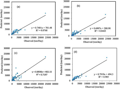
The temporal variation in observed and predicted SSL values are illustrated in Fig. 2(a)–(d). The figure shows that the RS estimates were closer to the corresponding observed values than those of the other models. Among the models, the RF model produced the poorest predictions, confirming. the results in Table 10. This can be further seen in the scatter plots of observed and predicted SSL in Fig. 3(a)–(d) using data from 2002 to 2010.

Figure 2. Temporal variation in observed and predicted suspended sediment load for the testing phase: (a) SVM_RBF, (b) SVM-NPK, (c) RF and (d) RS.

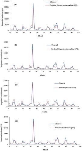
Figure 3. A comparison between observed and predicted suspended sediment load for the testing phase: (a) SVM-RBF, (b) SVM-NPK, (c) RF and (d) RS.

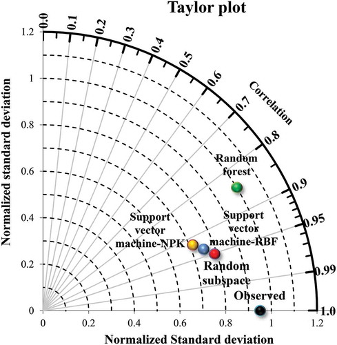
To further analyse the models’ performance, a Taylor plot was constructed (Fig. 4). This plot revealed that the RS model had the highest correlation coefficient followed by the SVM-RBF, SVM-NPK and RF. Also, the normalized standard deviation values show that the RF model had a standard deviation that closely matched that of the observed data.

Figure 4. Taylor plot for comparison of models’ prediction performance.

Although some models such as SVM and RF have performed successfully in SSL prediction in previous studies (Francke et al. 2008, Lafdani et al. 2013), in the present study, the new RS model outperformed the other models including SVM-RBF, SVM-NPK and RF. This occurred for a number of reasons. First, a random subspace model has a hybrid construction of the base learners which led to smaller error rates and enhanced noise insensitivity Second, RF hybrid models, unlike other hybrid models, use modified feature spaces to build hybrids of learners (Panov and Dzeroski 2007). Third, in the model combination phase, the RS model benefits from weighted majority voting (Neo and Ventura 2012). Weighted majority voting is a weighting factor that is used to reduce the error of the random subspace model, thus, the negative impact of poor base-learners on predictive capability can be omitted.

Although SVM is one of the most popular types of AI models because its predictive power has been proven in previous work (Lafdani et al. 2013, Zounemat-Kermani et al. 2016), the model suffers from a number of weaknesses, including: (a) the kernel function can be sensitive to over-fitting the model selection criterion (Cawley and Talbot 2010); (b) the loss function does not have an obvious statistical interpretation; and (c) in many classification problems the probability of class membership is required because a method such as kernel logistic regression, instead of post-processing output of the SVM, should be used. A random forest model also has some disadvantages: (i) the model is prone to errors in classification owing to differences in perceptions and the need to apply statistical tools; (ii) the module has high complexity, particularly if many values are uncertain; and (iii) the model is unwieldy.

The meta-heuristic algorithms overcome the weaknesses of the classic ANFIS model (Khosravi et al. 2018a). Thus, we recommend that new hybrid algorithms of ANFIS with meta-heuristic algorithms such as invasive weed optimization (IWO), differential evolution (DE), firefly algorithm (FA), particle swarm optimization (PSO) and bees algorithm (BA) should be investigated for SSL prediction. Also, we make two further recommendations: (a) that daily, weekly, monthly and seasonal datasets be considered as input variables to determine which period is the best combination for prediction of suspended sediment load; and (b) that rainfall intensity is included as an additional input variable due to its control on hillslope erosion, river discharge and thus suspended sediment loads in catchments.

Overall, our results reveal that RS models have great potential in data poor watersheds, such as the one studied here, to produce strong predictions of suspended load based on monthly records of river discharge, rainfall depth and river stage alone. This type of data driven model could complement existing process-based models in well gauged watersheds to recognize patterns within collected data that could unveil critical details about behavior, reveal previously unsuspected environmental relationships, or mitigate uncertainty in model estimates. In data poor watersheds, especially in developing nations where technical skills and understanding of the processes occurring in the watershed may be lacking, RS models could even be used alone or replace process-based models, because they represent well the highly stochastic behavior of sediment transport and are inexpensive to build and run. Future work should focus on testing artificial intelligence models developed in one watershed on measured suspended loads in others to reveal how widely the approach can be applied and how the performance of different algorithms varies.

9 Conclusion

The accurate prediction of suspended sediment load is important for understanding changes in reservoir storage capacity, river morphology, water quality and in the transport of non-point source pollution. Due to the non-linear nature of suspended sediment load in a river, the application of data mining and machine learning algorithms in its prediction has increased. In the present study, the suspended sediment load of Haraz River in the north of Iran was predicted using a new artificial intelligence model called random subspace (RS) and its predictive capabilities compared with two popular models; random forest (RF) and support vector machine (SVM) using radial bases function (RBF) and normalized polynomial kernels (NPK). The input variables were river discharge (Q), Q with one month lag time (Q-1), water stage (S), water stage with 1 month lag time (S-1), rainfall depth (R), rainfall with 1 month lag time (R-1), suspended sediment load (SSL), and SSL with 1 month lag time (SSL-1).

The results showed that the RS model provided a superior predictive accuracy to SVM-RBF, SVM-NPK and RF, which corresponded to very good, good, satisfactory and unsatisfactory accuracies in SSL prediction. The RBF kernel performed better than the NPK in SVM application. Changes in suspended sediment load were most closely related to changes in Q followed by S, SSL-1, Q-1, S-1, R-1 and R. Predictive capability was most sensitive to the gamma and epsilon in SVM models, maximum depth of tree and number of feature in RF models, classifier type, and number of tree and subspace size in RS models. The results show that RS models have great potential in data poor watersheds, such as the one studied here, to produce strong predictions of suspended load based on river discharge, rainfall depth and river stage data alone.

Acknowledgements

We would like to thank the editor in chief Prof. Attilio Castellarin, co-editor Dr Stacey Archfield, associate editor Dr Prashant Srivastava and three anonymous reviewers for their invaluable comments and suggestions which have improved the quality of the paper.

Disclosure statement

No potential conflict of interest was reported by the authors.

References

- Ahmadi, H., 2010. Applied Geomorphology. Vol. 1. Tehran, Iran: Tehran university press, 688.
- Ali, G. and Abbas, S., 2013. Exploring CO2 sources and sinks nexus through integrated approach: insight from Pakistan. Journal of Environmental Informatics, 22, 112–122. doi:10.3808/jei.201300250
- Ayele, G.T., et al., 2017. Stream flow and sediment yield prediction for watershed prioritization in the Upper Blue Nile River Basin, Ethiopia. Water, 9,782. doi:10.3390/w9100782
- Aytek, A. and Kisi, O., 2008. A genetic programming approach to suspended sediment modeling. Journal of Hydrology, 351 (3–4), 288–298. doi:10.1016/j.jhydrol.2007.12.005
- Azamathulla, H.M. and Wu, F.C., 2011. Support vector machine approach for longitudinal dispersion coefficients in natural streams. Applied Soft Computing, 11 (2), 2902–2905. doi:10.1016/j.asoc.2010.11.026
- Bathrellos, G.D., et al., 2017. Suitability estimation for urban development using multi-hazard assessment map. Science of the Total Environment, 575, 119–134. doi:10.1016/j.scitotenv.2016.10.025
- Boskidis, I., et al., 2012. Hydrologic and water quality modeling of Lower Nestos River Basin. Water Resource Management, 26 (10), 3023–3051. doi:10.1007/s11269-012-0064-7
- Breiman, L., 2001. Random forests. Machine Learning, 45 (1), 5–32. doi:10.1023/A:1010933404324
- Breiman, L., et al., 1984. Classification and regression trees. Belmont, CA: Wadsworth.
- Bui, D.T., Pradhan, B., Lofman, O., and Revhaug. I., 2012. Landslide susceptibility assessment in vietnam using support vector machines, decision tree, and Naive Bayes Models. Mathematical Problems in Engineering. ID 974638. https://ind01.safelinks.protection.outlook.com/?url=https%3A%2F%2Fdoi.org%2F10.1155%2F2012%2F974638&data=02%7C01%7Csathyan.dhanasekaran%40integra.co.in%7C75e2d51dcc1f473f4d9408d819c8ca92%7C70e2bc386b4b43a19821a49c0a744f3d%7C0%7C0%7C637287697474910233&sdata=O0o1Ot73VPFOiIdmBkusL8Bfn8VAePGnivRt%2Fxk%2BBAo%3D&reserved=0.
- Bui, D.T., et al., 2016. Hybrid artificial intelligence approach based on neural fuzzy inference model and metaheuristic optimization for flood susceptibility modeling in a high-frequency tropical cyclone area using GIS. Journal of Hydrology, 540, 317–330. doi:10.1016/j.jhydrol.2016.06.027
- Cawley, G.C. and Talbot, N.L.C., 2010. Over-fitting in model selection and subsequent selection bias in performance evaluation. Journal of Machine Learning Research, 11, 2079−2107.
- Chapi, K., et al., 2017. A novel hybrid artificial intelligence approach for flood susceptibility assessment. Environmental Modeling and Software, 95, 229–245. doi:10.1016/j.envsoft.2017.06.012
- Chiang, J.-L. and Tsai, Y.-S., 2011. Suspended sediment load estimate using support vector ma-chines in Kaoping river basin. Consum. Electron. Commun. Networks (CECNet). In: 2011 Int. Conf, Xianning, China, 1750–1753.
- Choubin, B., et al., 2018. River suspended sediment modelling using the CART model: A comparative study of machine learning techniques. Science of the Total Environment, 615, 272–281. doi:10.1016/j.scitotenv.2017.09.293
- Cigizoglu, H.K., 2002. Suspended sediment estimation and forecasting using artificial neural networks. Turkish Journal of Engineering and Environmental Sciences, 26, 15–25.
- Cigizoglu, H.K., 2004. Estimation and forecasting of daily suspended sediment data by multi-layer perceptrons. Advances in Water Resources, 27 (2), 185–195. doi:10.1016/j.advwatres.2003.10.003
- Çimen, M., 2016. Estimation of daily suspended sediments using support vector machines. Hydrological Science Journal, 53 (3), 656–666. doi:10.1623/hysj.53.3.656
- Dai, S.B. and Lu, X.X., 2010. Sediment deposition and erosion during the extreme flood events in the middle and lower reaches of the Yangtze River. Quaternary International, 226 (1–2), 4–11. doi:10.1016/j.quaint.2010.01.026
- Dawson, C.W., et al., 2006. Flood estimation at ungauged sites using artificial neural networks. Journal of Hydrology, 319 (1–4), 391–409. doi:10.1016/j.jhydrol.2005.07.032
- Dibike, Y.B., et al., 2001. Model induction with support vector machine: introduction and application. Journal of Computing in Civil Engineering, 15 (3), 208–216. doi:10.1061/(ASCE)0887-3801(2001)15:3(208)
- Dixon, B. and Candade, N., 2008. Multispectral landuse classification using neural networks and support vector machines: one or the other, or both? International Journal of Remote Sensing, 29 (4), 1185–1206. doi:10.1080/01431160701294661
- Fan, X., et al., 2012. Sediment rating curves in the Ningxia-Inner Mongolia reaches of the upper Yellow River and their implications. Quaternary International, 282, 152–162. doi:10.1016/j.quaint.2012.04.044
- Francke, T., L´opez-Tarazon, J.A., and Schroder, B., 2008. Estimation of suspended sediment concentration and yield using linear models, random forests and quantile regression forests. Hydrological Process, 22, 4892–4904. doi:10.1002/hyp.7110
- Hamel, P., et al., 2017. Sediment delivery modeling in practice: comparing the effects of watershed characteristics and data resolution across hydroclimatic regions. Science of the Total Environment, 580, 1381–1388. doi:10.1016/j.scitotenv.2016.12.103
- Heng, S. and Suetsugi, T., 2014. Comparison of regionalization approaches in parameterizing sediment rating curve in ungauged catchments for subsequent instantaneous sediment yield prediction. Journal of Hydrology, 512, 240–253. doi:10.1016/j.jhydrol.2014.03.003
- Ho, T.K., 1995. Random Decision Forests (PDF). In: Proceedings of the 3rd International Conference on Document Analysis and Recognition, 14–16 August 1995 Montreal, QC, 278–282.
- Ho, T.K., 1998. The random subspace method for constructing decision forests. IEEE Transactions on Pattern Analysis and Machine Intelligence, 20 (8), 832–844. doi:10.1109/34.709601
- Jain, S.K., 2001. Development of integrated sediment rating curves using ANNs. Journal of Hydraulic Engineering, ASCE, 127 (1), 30–37. doi:10.1061/(ASCE)0733-9429(2001)127:1(30)
- Jha, S.K. and Bombardelli, F.A., 2011. Theoretical/numerical model for the transport of non-uniform suspended sediment in open channels. Advances in Water Resources, 34 (5), 577–591. doi:10.1016/j.advwatres.2011.02.001
- Jie, L.C. and Yu, S.T., 2011. Suspended sediment load estimate using support vector machines in Kaoping River basin. IEEE Xplore Conferences. doi:10.1109/CECNET.2011.5769267
- Khosravi, K., et al., 2016. A GIS-based flood susceptibility assessment and its mapping in Iran: a comparison between frequency ratio and weights-of-evidence bivariate statistical models with multi-criteria decision-making technique. Natural Hazards, 83 (2), 1–41. doi:10.1007/s11069-016-2357-2
- Khosravi, K., Panahi, M., and Tien Bui, D., 2018c. Spatial prediction of groundwater spring potential mapping based on an adaptive neuro-fuzzy inference system and metaheuristic optimization. Hydrology and Earth System Science, 22 (9), 4771–4792. doi:10.5194/hess-22-4771-2018
- Khosravi, K., et al., 2018a. A comparative assessment of decision trees algorithms for flash flood susceptibility modeling at Haraz watershed, northern Iran. Science of the Total Environment, 627, 744–755. doi:10.1016/j.scitotenv.2018.01.266
- Khozani, Z., et al., 2019. Determination of compound channel apparent shear stress: application of novel data mining models. Journal of Hydroinformatics, 21 (5), 798–811. doi:10.2166/hydro.2019.037
- Kira, K. and Rendell, L., 1992. A practical approach to feature selection. In: Proceedings of the Ninth International Workshop on Machine Learning, San Francisco, CA, US, 249–256.
- Kisi, O., 2004. Multi-layer perceptions with Levenberg-Marquardt training algorithm for suspended sediment concentration prediction and estimation. Hydrolological Science Journal, 49 (6), 1025–1040.
- Kisi, O., et al., 2012. Suspended sediment modeling using genetic programming and soft computing techniques. Journal of Hydrology, 450, 48–58. doi:10.1016/j.jhydrol.2012.05.031
- Lafdani, E.K., Nia, A.M., and Ahmadi, A., 2013. Daily suspended sediment load prediction using artificial neural networks and support vector machines. Journal of Hydrology, 478, 50–62. doi:10.1016/j.jhydrol.2012.11.048
- Legates, D.R. and McCabe, G.J., 1999. Evaluating the use of “goodness-of-fit” measures in hydrologic and hydroclimatic model validation. Water Resources Research, 35 (1), 233–241. doi:10.1029/1998WR900018
- Li, B., et al., 2016. Comparison of random forests and other statistical methods for the prediction of Lake water level: a case study of the Poyang Lake in China. Hydrology Research. doi:10.2166/nh.2016.264
- Lin, J.Y., Cheng, C.T., and Chau, K.W., 2006. Using support vector machines for long-term discharge prediction. Hydrological Science Journal, 51 (4), 599–612. doi:10.1623/hysj.51.4.599
- Mao, L. and Carrillo, R., 2017. Temporal dynamics of suspended sediment transport in a glacierized Andean basin. Geomorphology, 287, 116–125. doi:10.1016/j.geomorph.2016.02.003
- Melesse, A.M., et al., 2011. Suspended sediment load prediction of river systems: an artificial neural network approach. Agricultural Water Management, 98 (5), 855–866. doi:10.1016/j.agwat.2010.12.012
- Mert, A., Kılıç, N., and Bilgili, E., 2016. Random subspace method with class separability weighting. Expert Systems, 33 (3), 275–285. doi:10.1111/exsy.12149
- Mielniczuk, J. and Teisseyre, P., 2014. Using random subspace method for prediction and variable importance assessment in linear regression. Computational Statistics & Data Analysis, 71, 725–742. doi:10.1016/j.csda.2012.09.018
- Moriasi, D.N., et al., 2007. Model evaluation guidelines for systematic quantification of accuracy in watershed simulations. Transactions of the ASABE, 50 (3), 885–900. doi:10.13031/2013.23153
- Neo, T.K.C. and Ventura, D., 2012. A direct boosting algorithm for the k-nearest neighbor classifier via local warping of the distance metric. Pattern Recognition Letters, 33 (1), 92–102. doi:10.1016/j.patrec.2011.09.028
- Nourani, V., 2009. Using artificial neural networks (ANNs) for sediment load forecasting of Talkherood River mouth. Journal of Urban and Environmental Engineering, 3 (1), 1–6. doi:10.4090/juee.2009.v3n1.001006
- Onan, A., 2015. Classifier and feature set ensembles for web page classification. Journal of Information Science. doi:10.1177/0165551515591724
- Panov, P. and Dzeroski, S., 2007. Combining bagging and random subspaces to create better ensembles. In: 7th Int Sym on Intell Data Anal Proc, Germany, 118–129.
- Partal, T. and Cigizoglu, H.K., 2008. Estimation and forecasting of daily suspended sediment data using wavelet-neural networks. Journal of Hydrology, 358 (3–4), 317–331. doi:10.1016/j.jhydrol.2008.06.013
- Pham, B.T., et al., 2016. Evaluation of predictive ability of support vector machines and naive Bayes trees methods for spatial prediction of landslides in Uttarakhand state (India) using GIS. Journal of Geomatics, 10 (1), 71–79.
- Pham, B.T., et al., 2017b. Hybrid integration of multilayer perceptron neural networks and machine learning ensembles for landslide susceptibility assessment at Himalayan area (India) using GIS. Catena, 149, 52–63. doi:10.1016/j.catena.2016.09.007
- Pham, B.T., Khosravi, K., and Prakhsh, I., 2017a. Application and comparison of decision tree-based machine learning methods in landside susceptibility assessment at Pauri Garhwal Area, Uttarakhand, India. Environmental Processes, 4 (3), 711–730. doi:10.1007/s40710-017-0248-5
- Pradhan, B., 2013. A comparative study on the predictive ability of the decision tree, support vector machine and neuro-fuzzy models in landslide susceptibility mapping using GIS. Computer and Geoscience, 51, 350–365. doi:10.1016/j.cageo.2012.08.023
- Rajaee, T., 2011. Wavelet and ANN combination model for prediction of daily suspended sediment load in rivers. Science of the Total Environment, 409 (15), 2917–2928. doi:10.1016/j.scitotenv.2010.11.028
- Sharafati, A., et al., 2019. The potential of novel data mining models for global solar radiation prediction. International Journal of Environmental Science and Technology, 1–18. doi:10.1007/s13762-019-02344-0
- Shkurin, A., 2015. Water quality analysis using machine learning algorithms. Bachelor’s Thesis in Environmental Engineering. MAMK University of applied science, 54.
- Tang, X., et al., 2014. Phosphorus storage dynamics and adsorption characteristics for sediment from a drinking water source reservoir and its relation with sediment compositions. Ecological Engineering, 64, 276–284. doi:10.1016/j.ecoleng.2014.01.005
- Tehrany, M.S., Pradhan, B., and Jebur, M.N., 2014. Flood susceptibility mapping using a novel ensemble weights-of-evidence and support vector machine models in GIS. Journal of Hydrology, 512, 332–343. doi:10.1016/j.jhydrol.2014.03.008
- Tien Bui, D., et al., 2012. Landslide susceptibility assessment in Vietnam using support vector machines, decision tree, and Naive Bayes Models. Mathematical Problems in Engineering, 26. doi:10.1155/2012/974638
- Vapnik, V., 1995. The Nature of Statistical Learning Theory. New York: Springer.
- Vapnik, V., Golowich, S.E., and Smola, A.J., 1997. Support vector method for function approximation, regression estimation and signal processing. In: NIPS’96: Proceedings of the 9th international conference on neural information processing systems, December 1996, 281–287.
- Vigiak, O., et al., 2017. Modelling sediment fluxes in the Danube River Basin with SWAT. Science of the Total Environment, 599, 992–1012. doi:10.1016/j.scitotenv.2017.04.236
- Wenske, D., et al., 2012. Assessment of sediment delivery from successive erosion on stream-coupled hillslopes via a time series of topographic surveys in the central high mountain range of Taiwan. Quaternary International, 263, 14–25. doi:10.1016/j.quaint.2011.02.018
- Zounemat-Kermani, M., et al., 2016. Evaluation of data driven models for river suspended sediment concentration modeling. Journal of Hydrology, 535, 457–472. doi:10.1016/j.jhydrol.2016.02.012