Forecasting annual precipitation to improve the operation of dams in the Comahue region, Argentina

ABSTRACT

This paper attempts to design statistical models to forecast annual precipitation in the Neuquen and Limay river basins in the Comahue region of Argentina. These forecasts are especially useful as they are used to better organize the operation of hydro-electric dams, the agriculture in irrigated valleys and the safety of the population. In this work, multiple linear regression statistical models are built to forecast mean annual rainfall over the two river basins. Since the maximum precipitation occurs in the winter (June–August), forecasting models have been developed for the beginning of March and for the beginning of June, just before the rainy season starts. The results show that the sea-surface temperatures of the Indian and Pacific oceans are good predictors for March models and explain 42.8% of the precipitation index variance. The efficiency of the models increases in June, adding more predictors related to the autumn circulation.

KEYWORDS:

• statistical forecast
• annual precipitation
• Argentina
• hydro-electric energy

Editor A. Castellarin Associate editor X. Sun

1 Introduction

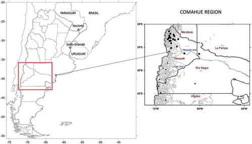
The Comahue region is located in the extreme north of Argentinean Patagonia (Fig. 1). The Andes Mountains lie along the western part of the area. This region is crossed by three important rivers: the Neuquén, Limay and Negro, the first two being tributaries of the third. It drains an area of 140 000 km² and covers almost the entire territory of the Province of Neuquen and part of Rio Negro and Buenos Aires provinces. The Neuquen River, with a mean flow of 280 m³/s, drains an area of 30 000 km², while the Limay River flow is 650 m³/s in an area of 56 000 km². Both make up the Negro River that drains a basin of 116 000 km², with a mean flow of 930 m³/s. The Negro River is the largest water course that is entirely in Argentina, with important potential uses that are planned for the future.

Figure 1. Area of study and stations used (circles: Neuquen River basin; triangles: Limay River Basin).

The prediction of annual precipitation in the Comahue region enables decision-makers to better plan activities that result in economic improvements (production of hydro-electric energy and agriculture) and the safety of the population. However, the importance of energy production lies in the fact that the Argentine Interconnection System (SADI) transports energy from the places of production through the national territory and to bordering countries, such as Paraguay, Brazil and Uruguay.

Although the largest percentage of hydro-electric energy is generated by the Yacireta and Salto Grande bi-national power plants, the hydro-electric production of the Comahue region constitutes about 15–25% of the total of the country and generates approx. USD300 million per year.

Precipitation in the Comahue region has a marked annual cycle, with a maximum in the winter (June–August), and the river flows are highly dependent on winter precipitation. In fact, temporal series derived from principal component analysis that was applied to mean annual precipitation was correlated with the mean annual flow during the hydrological year in each river, showing that positive rainfall anomalies near the Andes Mountains determined positive river flow anomalies (González et al. 2015). A very detailed account of the main features of the climate and precipitation over the Andes Mountains in South America is given by Garreaud (2009).

The rainy season begins in May and ends in October. When the height of the rivers in the autumn is close to the maximum allowed, it is convenient to turbinate part of the water to generate electricity. If this is not done, there is a risk that the dams will be damaged and endangering the populations located downstream. On the other hand, when the water is well below the maximum allowed level in the autumn, there is the possibility of not generating the necessary energy, especially if the winter (rainy season) is drier than normal.

Additionally, a decrease in annual accumulated precipitation has been observed in the west of the region, which clearly provides less flow to the rivers (Vera and Camilloni 2006, Aravena and Luckman 2009, Garreaud et al. 2013). This reduction is mainly observed when considering the stations located in the west in the high mountains, but it is not detected in the region to the east of the Andes. A decrease in annual precipitation of around 38 mm/year was observed in the high mountains of the Limay basin and 40 mm/year in the Neuquen during the period 2001–2016, both with 95% statistical significance (González et al. 2019). However, the precipitation presents a great inter-annual variability, with variations of up to 100% between 1 year and another, superimposed on an important decadal variability (UNCCF, 3CN 2015).

In general, dynamical models fail to predict rainfall in this region because of their low spatial resolution (e.g. Rostkier-Edelstein et al. 2010, Diro et al. 2012, Yuan et al. 2017), so statistical methods enable one to model precipitation using the knowledge of its behaviour in the past. In this work, an annual precipitation forecasting scheme is derived for the Comahue region using statistical methodologies. Therefore, the need to have a statistical forecast of annual rainfall before autumn (March) and when the rainy season has just begun (June), is of great value for the operation of dams, the economy and security. To do this, it is relevant to detect the climate atmospheric and oceanic forcings, which influence the annual precipitation. Some studies have been previously developed in the Comahue area (e.g. González and Vera 2010, González 2013, Scarpati et al. 2014, Garbarini et al. 2016), the inter-annual variability rainfall patterns have been studied and, in some cases, winter rainfall forecasting schemes using statistical methods have been derived. It was detected that most dry and wet periods persist for less than 3 months in the Limay and Neuquen river basins. Furthermore, an increase in rainfall variability over time was observed in the Limay River basin, but it was not detected in the Neuquen River basin, and there was a tendency for wet periods to take place in El Niño years (and dry periods in La Niña years) in both basins (González and Dominguez 2012). A relevant relationship was detected between the inter-annual variability of mean flows and cumulative rainfall during the year in both basins (Romero and González 2016) and positive rainfall anomalies near the Andes Mountains determined positive river flow anomalies (González et al. 2015). General features of the rainy season and precipitation excess or deficit were analysed using the standardized precipitation index for a 6-month period in the Neuquen River basin and a prediction scheme for that index was derived (González 2015). This work addresses the problem of predicting the total volume of rain that contributes to the flow and that can be used as an input in the hydrological models for the estimation of flow and therefore the possible hydro-electric energy associated with it.

The El Niño-Southern Oscillation (ENSO) is one of the main factors that influences precipitation in Comahue (Garbarini et al. 2016) the same as in some other regions of southern South America (e.g. Ropelewski and Halpert 1987, 1989, Karoly 1989, Grimm et al. 2002, Vera et al. 2004, Barreiro 2010, Penalba and Rivera 2016). The linkage mechanism is well explained by Mo (2000) and Nogues Paegle and Mo (2002). However, there are other factors that affect precipitation in South America, such as, for example, the South American Mode (e.g. Silvestri and Vera 2003, Reboita et al. 2009), or the sea-surface temperature anomalies in the Indian Ocean. In this case, the Indian Ocean Dipole (IOD) (Saji et al. 1999) determines a teleconnection pattern that induces an anomalous rainfall dipole, with decreased precipitation in northern South America (and enhanced precipitation in southern parts) (Chan et al. 2008), when the positive phase is present. Another pattern, known as the Indian Ocean basin-wide warming and closely related to ENSO (Klein et al. 1999), also affects rainfall in South America (Taschetto and Ambrizzi 2012). But ENSO and IOD seemed not to be always independent: Wang et al. (2016) studied the forcing mechanisms of IOD in the absence of an ENSO signal and demonstrated that ENSO is not fundamental for the existence of IOD.

All these factors are considered for building a multiple linear regression (MLR) model to predict mean annual precipitation in the Comahue region. Annual precipitation is relevant data for the estimation of river flow and, consequently, for the efficient management of hydro-electric dams, which is why its prognosis is addressed in this study.

2 Data and methodology

The area of study comprises the Limay and Neuquén river basins in the Comahue area of Argentina (Fig. 1). Annual rainfall data for 30 stations from different sources (Argentinian National Weather Service, Ministry of Water Resources of the Nation and the Interjurisdictional Authority of Limay, Neuquen and Negro River basins) for the period 1985–2012 were used as a training sample to build the model. The verification was done using data from the period 2013–2017. Data quality was carefully verified: only stations with less than 10% of missing values were used and, in cases of extreme precipitation, the data were verified by comparing with those of nearby stations.

Meteorological variables used in this study are monthly sea-surface temperature (SST), 500 hPa (G500) geopotential height, zonal (U) and meridional (V) winds at 850 hPa and precipitable water (PW) from the National Center of Environmental Prediction (NCEP) reanalysis (Kalnay et al. 1996).

The prediction models are derived using the MLR technique. In order to measure the predictive accuracy, three statistics are calculated: adjusted R² (AdjR²; Theil 1961), cross-validation index (CVI; Efron and Gong 1983, Michaelson 1987, Efron and Tibshirani 1993, Elsner and Schmertmann 1994) and the Akaike information criterion (AIC; Akaike 1974).

The coefficient of determination, R², is the square of the correlation between the actual and the predicted values and represents the proportion of variance in the forecast variable that is explained by MLR model. It is not a good measure of forecasting skill because adding any variable tends to increase R² even if the variable is irrelevant. Therefore, AdjR² was designed to overcome this problem:

(1) $\mathrm{A}\mathrm{d}\mathrm{j}{\mathrm{R}}^2=1-\left(1-{\mathrm{R}}^2\right)\left(N-1\right)/\left(N-k-1\right)$(1)

where N is the number of observations and k is the number of predictors. Using this statistic, the best model will be the one with the largest AdjR².

The most frequently used cross-validation procedure is known as leave-one-out cross-validation, in which the fitting procedure is repeated n times, each time with a sample of size n–1, where one of the observations is left out in each replication of the fitting process (Wilks 2011). This process was repeated for every year and a cross-validation series was built with all the validated values. The error is the residual from the fitting model, computed as:

(2) $E_i=\mathrm{I}{\mathrm{E}}_i-\mathrm{I}{\mathrm{E}}_{pi}$(2)

where $\mathrm{I}{\mathrm{E}}_i$ is the actual value and $\mathrm{I}{\mathrm{E}}_{pi}$ is the predicted value for each year i. Note that the ith year was not used in estimating the value of $\mathrm{I}{\mathrm{E}}_{pi}.$ The CVI is calculated as the mean square error (MSE) from $E_i$:

(3) $\mathrm{C}\mathrm{V}\mathrm{I}=\mathrm{M}\mathrm{S}\mathrm{E}\left(E_1;E_2;E_3;\dots ;E_n\right)$(3)

(4) $\mathrm{C}\mathrm{V}\mathrm{I}=\sum _{i=1}^N{\left[Ei\right]}^2/N$(4)

This method is generally robust in the presence of long-term climate variability and is used especially when the amount of data is not so large that one can divide the dataset into training and verification subsets. The best model selected will be the one with the smallest CVI. The consideration of the CVI statistic is important in this work because a small CVI guarantees the stability of the model. In this paper, the cross-validation method is applied to IE for the period 1985–2012 in which out of 28 years, 27 are used for calibration and the process is repeated 28 times. Since the lag-1 autocorrelation coefficient is 0.1 (not significant), the cross-validation can be repeated with no longer left out periods. As, when the cross-validation method is applied, the coefficients of all the models remained similar, there is no evidence of numerical instability.

The AIC is defined (in the case of the least-squares estimation with normally distributed errors) as:

(5) $\mathrm{A}\mathrm{I}\mathrm{C}=N\cdot \mathrm{l}\mathrm{o}\mathrm{g}\left(\mathrm{S}\mathrm{S}\mathrm{E}/N\right)+2\left(k+2\right)$(5)

where SSE is the minimum sum of square errors. The reason for the second term is that there are (k + 2) parameters in the model (k predictors, the intercept and the variance of residuals). The model with minimum AIC is often the best model.

The skill of the forecast is also proved using contingency tables, which compare the categorized observed precipitation with the categorized forecasted IE derived from cross-validation. Besides, a chi-square (χ²) test is applied to detect if observed and forecasted IE differ significantly. Some measures, derived from contingency tables (Wilks 2011), are calculated for above-normal and below-normal cases. The hit rate (H) or the right proportion is the fraction of all the cases when the categorical forecast correctly anticipated the subsequent event. The probability of detection (POD) is defined as the fraction of those occasions when the forecasted event occurred where it was also forecasted. The false alarm ratio (FAR) is the proportion of forecasted events that fail to happen.

3 Results and discussion

3.1 Precipitation index definition

For each one of the stations, the 33rd and 66th percentiles of cumulative annual precipitation are used as thresholds to define if the year was dry (annual precipitation lower than 33rd percentile), wet (annual precipitation greater than 66th percentile) or normal (between 33rd and 66th percentiles). Each of the Limay and Neuquen river basins is classified as dry, wet or normal if most of the stations (more than 60%) in the basin are classified as dry, wet or normal, respectively. It was found that in a basin for a given year, some stations are classified as normal and others as wet or dry. In general, most of the stations in a basin are classified as wet and some others as normal, or most of the stations are dry while others are normal; however, stations are not classified as wet and some others as dry in the same year, indicating that the whole basin tends to register the same water condition. Indeed, the annual rainfall in each of the stations located in the Limay River Basin is significantly correlated (95% confidence using Student’s t test) with 90% of the remaining stations, while in the Neuquen River Basin the correlation is 85%.

Wet years derived using this methodology are 1993, 1994, 1997, 2001, 2002, 2004, 2005, 2006 and dry years are 1988, 1989, 1996, 1998, 2003, 2007, 2010, 2011, 2012. The classification method is fully detailed in González et al. (2017).

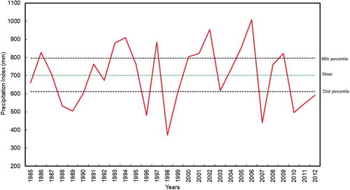
A related precipitation index (IE) is defined as:

(6) $\mathrm{I}\mathrm{E}=\left(\mathrm{P}\mathrm{R}\mathrm{N}+\mathrm{P}\mathrm{R}\mathrm{L}\right)/2$(6)

where PRN and PRL are the areal annual precipitation in the Neuquen and Limay river basins, respectively; this represents the mean annual accumulated precipitation in both basins. Figure 2 shows the inter-annual variability of this index.

Figure 2. Evolution of the precipitation index, IE, used to represent the annual precipitation averaged over the Neuquen and Limay river basins.

3.2 Annual precipitation prediction

Precipitation has a maximum in the winter in both basins (Fig. 3), so it is desirable that its forecast is available before winter. That is the reason why some statistical models are designed to predict IE in March. Then, when the rainy season has just begun, a new forecast in early June probably improves the previous estimate.

Figure 3. Mean monthly precipitation (mm) in the Limay (dashed line) and Neuquen (solid line) river basins.

To design the statistical models, some predictors must be defined. To do so, composite fields are built for wet and dry years (as detailed in the previous section) for several meteorological variables in December–February (DJF) and March–May (MAM) previous to winter. The variables used are SST, G500, U, V and PW, and the anomalies are computed from the series without trend. Subsequently, the difference between the composite fields for wet and dry years is calculated. The predictors are defined taking into account the areas where the difference between wet and dry years is high and significant (95% confidence level) using the Student t test.

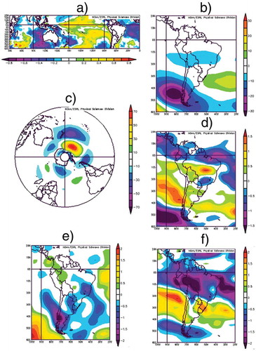
Figure 4(a)–(f) shows the difference composites for SST, G500, U, V and PW in DJF prior to predicted winter precipitation and Fig. 5(a)–(f) shows the same for MAM. The areas with positive (orange) and negative (purple) high values represent the major differences between the wet and dry years. These areas enable the definition of the predictors that will be used. Years with precipitation greater than normal are associated with the negative ENSO phase and negative SST anomalies in the eastern Indian Ocean (Fig. 4(a)), anticyclonic anomalies over the Comahue area extending to the South Pole (Fig. 4(b) and (c)), mean latitude westerlies (40°S) intensified in the Pacific Ocean and weakened in the Atlantic Ocean (Fig. 4(d)), and meridional wind anomalies from the north (Fig. 4(e)), even when precipitable water is normal over the basins (Fig. 4(f)) in the previous summer. Some features in the previous autumn favour precipitation: a positive ENSO phase (Fig. 5(a)), cyclonic anomalies over the study region (Fig. 5(b) and (c)), intensified western zonal wind over the region (Fig. 5(d)) and the Pacific and the Atlantic oceans, and northern meridional wind component (Fig. 5(e)) with positive PW anomalies (Fig. 5(f)) over the basins. Therefore, cyclonic circulation anomalies generate air rise that, together with the availability of water in the atmosphere, produces higher precipitation values. Table 1 summarizes all the predictors defined and the correlation between them and the IE index defined previously. Values greater than or equal to 0.37 are statistically significant at the 95% confidence level.

Table 1. Definition of predictors defined considering the areas with significant (95%) IE difference between wet and dry years (Figs. 4 and 5), averaged in DJF or MAM. The correlation between annual precipitation and the predictor is detailed in the last column. SST: sea-surface temperature; G500: geopotential height at 500 hPa.

Predictor	Variable	Predictor definition	Correlation between predictor and IE	Predictor	Variable	Predictor definition	Correlation between predictor and IE
S1p_djf	SST	(120°,75°W;5°N,5°S)	–0.41*	G4p_djf	G500	(115°,95°W; 44°,50°S)	–0.48 *
S2p_djf	SST	(76,74°W; 5°,10°S)	–0.46*	DIFG3G4	G500	G3p–G4p	0.54 *
S3p_djf	SST	(75°,72°W; 30°,25°S)	0.12	G5p_djf	G500	(90°,115°E; 35°,40°S)	–0.47 *
S4a_djf	SST	(65°,55°W; 45°,50°S)	0.17	G6p_djf	G500	(165°E,170°W;25°,35°S)	–0.47 *
S5a_djf	SST	(25°,10°W; 15°,20°S)	–0.34	DIFG5G6	G500	G5p–G6p	0.03
S6p_djf	SST	(110°,95°W;25°,30°S)	0.43 *	G7p_djf	G500	(20°,30°E; 50°,70°S)	–0.32
S7p_djf	SST	(125°,112°W;40°,45°S)	–0.38 *	G8p_djf	G500	(178°E,175°W;60°,80°S)	–0.08
S8p_djf	SST	(175°,160°W;5°N,0°S)	0.22	G9p_djf	G500	(90°,110°E; 65°,80°S)	0.05
S9p_djf	SST	(170°,160°W;21°,27°S)	0.37 *	DIFG8G9	G500	G8p–G9p	–0.22
S10p_djf	SST	(158°,155°W;28°,32°S)	0.39 *	G1p_mam	G500	(90°,73°W; 40°,51°S)	–0.01
S11i_djf	SST	(115°,106°E;16°,25°S)	–0.36	G1p_mam	G500	(180°,160°W;40°,55°S)	–0.09
S12i_djf	SST	(118°,115°E;30°,38°S)	–0.54 *	G1p_mam	G500	(178°,158°W; 70°,80°S)	0.18
S13i_djf	SST	(100°,85°E; 38°,47°S)	–0.35	U1p_djf	u850	(100°,82°W; 34°,42°S)	0.34
S14i_djf	SST	(70°,55°E; 14°,20°S)	–0.42 *	U2p_djf	u850	(96°,80°W; 52°,62°S)	–0.02
S15i_djf	SST	(50°,40°E; 30°,36°S)	0.22	U3a_djf	u850	(57°,46°W; 38°,42°S)	–0.31
S1a_mam	SST	(25°,5°W; 3°N,5°S)	–0.31	U4a_djf	u850	(43°,32°W; 43°,48°S)	–0.38 *
S2a_mam	SST	(30°,8°W; 15°,23°S)	–0.28	U1p_mam	u850	(85°,80°W; 27°,35°S)	0.45 *
S3p_mam	SST	(98°,88°W; 40°,48°S)	–0.33	U2p_mam	u850	(82°,74°W; 36°,41°S)	0.47 *
S4p_mam	SST	(180°,170°W;32°,40°S)	–0.29	U3p_mam	u850	(100°,78°W; 48°,58°S)	–0.22
S5p_mam	SST	(180°,160°E;3°N,3°S)	–0.16	V1_djf	v850	(65°,58°W; 12°,21°S)	0.54 *

*Correlation is significant at the 95% confidence level.

Figure 4. Difference between wet and dry years for (a) SST, (b and c) G500, (d) U, (e) V and (f) PW composites in DJF prior to predicted winter precipitation.

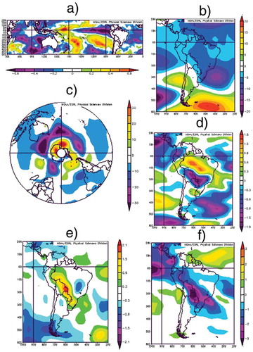
Figure 5. Difference between wet and dry years for (a) SST, (b and c) G500, (d) U, (e) V and (f) PW composites in MAM prior to predicted winter precipitation.

3.3 Statistical prediction models

Some groups of predictors are built following the criteria that they are significantly correlated with IE (p > 0.05) and they are uncorrelated with each other in order to avoid multi-collinearity which occurs when similar information is provided by two or more of the predictor variables in an MLR model. It is important to point out that correlation is not always causation but may be useful for selecting the best predictors. This is the reason why the different predictors used in this work are selected only if there is a physical relationship with precipitation.

Table 2 shows some sets of predictors used in this study. Each set is used to design an MLR using the backward stepwise method. This method starts considering all the predictors in a set and subtracts one predictor at a time. The method keeps the model if it improves the previous one and iterates until no further improvement. This methodology always leads to a good model although it is not certain to lead to the best one. Table 2 shows the model designed with each set of predictors and some statistics used to evaluate the model efficiency. The final model is constructed with 28 values and less than seven predictors in order to avoid overfitting. One of the models (Set 2) retains only DJF predictors while the others use DJF and MAM predictors. Therefore, the first can be used to predict IE in early March and the others in early June.

Table 2. Sets of independent potential predictors that are input into the models, the best model built for each set of predictors and the measure of accuracy given by CVI, AIC and AdjR² coefficients.

	Potential predictors	Best model (IE in mm)	CVI (mm^2)	AIC	AdjR^2
Set 1	S2p_djf	–209.8 S2p_djf – 59.3 S12i_djf + 4.1 G3p_djf – 64.6 V1_mam + 692.1	15649.8	267.5	0.607
	S12i_djf
	G3p_djf
	G4p_djf
	V1_mam
	S12i_djf
Set2	S1p_djf	–83.5 S12i_djf – 165.6 S1p_djf+694.7	16777.8	275.9	0.428
	G3p_djf
	V2p_djf
	U2p_mam
Set3	S6p_djf	56.1 U2p_mam +77.1 S6p_djf – 103 S7i_mam + 5.1 G3p_djf+696.7	17894.3	275.7	0.465
	S7i_mam
	G3p_djf
	PW2p_mam
	S10p_djf
Set 4	S7i_mam	49.8 PW2p_mam +109.3 S10p_djf – 135.9 S7i_mam – 3 G6p_djf + 693.4	13317.9	267.4	0.602
	G6p_djf
	V2p_mam
Set 5	DIFG3G4	1.8 DIFG3G4 – 159.1 S7i_mam + 65.6 U1p_mam + 108.8 S10p_djf + 693.3	11885.2	262.3	0.668
	S7i_mam
	U1p_mam
	S10p_djf

When N is large, the best model has the maximum AdjR² and the minimum CVI and AIC.

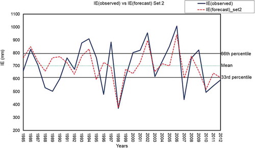
Figure 6 shows the comparison between observed and forecasted IE derived from the model using Set 2 predictors. It is important to point out that the forecasted IE values are the results of the application of the cross-validation method described previously in this section. Both predictors used in the model are defined in DJF and so IE can be forecasted in early March. The model only uses SST predictors (S12i_djf and S1p_djf), they are the mean SST values in the Indian Ocean (west Australia) and the Central Tropical Pacific Ocean. This model explains the 42.8% of the IE variance. The largest discrepancy between forecasted and observed IE is present in the years 1988–1990, 1996, 1997, 2000, 2001, 2005, 2009 and, in general, the model under-estimates the extreme values (Fig. 6). When converting to categorical forecasts 46.4% of the actual IE is well classified and 42.8% fails only in one category; meanwhile, 10.7% is wrongly classified (Table 3).

Table 3. Percentage of cases correctly classified by each set of independent potential predictors that differ in one category and those wrongly classified as above-normal, normal or below-normal using the different models.

	Correctly classified	Differ in one category	Wrongly classified
Set 2	46.4	42.8	10.7
Set 1	64.3	28.6	7.4
Set 3	60.7	35.7	3.6
Set 4	78.6	21.4	0
Set 5	67.8	28.6	3.6

Figure 6. Observed and forecasted IE (mm) using the best model derived from Set 2 (see Table 2). The prediction can be done in early March.

For this model, the values of POD, FAR and H obtained are, respectively, 0.50, 0.50 and 0.64 in the case of above-normal years and 0.56, 0.44 and 0.71 for below-normal years (Table 4). Additionally, forecasted and observed IE probability functions are calculated using cumulative frequency distributions and a χ² test was used to prove that they were significantly similar at the 95% confidence level. The efficiency of the model derived from Set 2 is very low because it detects only 50% of the above-normal cases, while FAR is too high.

Table 4. Probability of detection (POD), false alarm ratio (FAR) and hit rate (H) for above-normal and below-normal cases derived using the different models. Best scores are indicated in bold.

		Above-normal cases			Below-normal cases
Predictor period	Set	POD	FAR	H	POD	FAR	H
DJF	2	0.50	0.50	0.64	0.56	0.44	0.71
DJF-MAM	1	0.70	0.30	0.79	0.67	0.33	0.79
	3	0.70	0.30	0.79	0.67	0.33	0.79
	4	0.90	0.10	0.93	0.78	0.22	0.86
	5	0.80	0.20	0.86	0.67	0.33	0.79

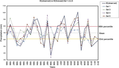
Figure 7 shows the observed and forecasted IE using the cross-validation method applied to the model derived from sets 1, 3, 4 and 5 of predictors. In these cases, the predictors selected by each model are defined in DJF and MAM, so they can be used to forecast IE in early June. These four models (in early June) improve the forecasted precipitation derived from Model 2 in early March. All the models use SST in the Indian and tropical Pacific oceans as predictors (S12i_djf, S7i_mam, S2p_djf, S1p_djf, S6p_djf, S10_djf). Models 3, 4 and 5 use a geopotential height predictor in the Pacific Ocean (G3p_djf, G6p_djf, DIFG3G4). Models 3 and 5 use zonal wind predictors (U2p_mam, U1p_mam). Model 1 includes meridional wind (V1_mam) and Model 4 precipitable water (Pw2p_mam) as predictors.

Figure 7. Observed and forecasted IE (mm) using the best model derived from sets 1, 3 4 and 5 (Table 2). The prediction can be done in early June.

The SST over the tropical Pacific and Indian oceans, geopotential height and zonal wind over the Pacific Ocean are predictors related to the wave train towards the east, associated with rainfall systems in the study area. In fact, a warming or cooling of some regions of the tropical oceans acts as a remote forcing and generates teleconnections. The SST anomalies in the tropical Pacific (ENSO) or Indian oceans generate a Rossby wave trend which propagates easterly and meridionally towards mid-latitudes from the tropical source (Kidson 1999, Mo 2000, Nogues Paegle and Mo 2002). This pattern, called the “Pacific South American Pattern”, is described by Mo (2000) when depicting the Southern Hemisphere climate. Other variables used as predictors are precipitable water and low-level meridional wind near the area of study. They are both related to moist air advection that can influence rainfall amounts through the low-level jet stream, which is a typical feature in warm season in subtropical Argentina, Paraguay and Bolivia (Salio et al. 2002). This pattern is associated with humidity advection from the north towards central Argentina.

The models derived from sets 1, 3, 4 and 5 (Table 2) of predictors explain the 60.7%, 46.5%, 60.2% and 66.8% of the IE variance, respectively. The model derived from Set 5 explains the maximum percentage of IE variance; it is the most stable as it has the minimum CVI and AIC. Tables 3 and 4 show the values of the statistics used to evaluate the accuracy of the predictions. Model 4 provides 78.6% of the cases well classified in above-and below-normal and normal categories and no cases were wrongly classified (Table 3). The number of cases well classified decreases when using models 1, 3 and 5. The forecast derived from Set 4 is the best in the case of years with precipitation above normal (POD: 90%, FAR: 10% and H: 93%), and below normal (POD: 78%, FAR: 22%, H: 86%). Models 1 and 3 have the least accuracy with H = 79% for above- and below-normal precipitation cases. Model 5 has better accuracy (H: 86%) for above-normal cases than for below-normal cases (H: 79%). The χ² test shows that observed and forecasted statistical distributions of IE values for the different models are significantly similar at the 95% confidence level. When the efficiencies of these models (with predictors defined in the summer and autumn before the rainfall season) are compared with the efficiency of Model 2 (with predictors defined only in the previous summer), a relevant improvement is detected. In early June, the rainy season has just begun but decision-makers can still use these forecasts properly.

The period 2013–2017 is used to prove the prognosis derived from each model (Fig. 8). Although the record is too short to compile statistics, the forecasts are shown as an example of application. Figure 8 shows the forecasted IE using the different models (top panel) and the comparison between the forecasted and the observed categories (bottom). The results are similar using the different models; IE in 2017 is wrongly forecasted for all the models except for Model 1. The IE category in years 2013, 2014 and 2015 is well forecasted with four of the five models. The accuracy of the models seems to be similar: in three of the 5 years, and IE is well forecasted. Although the verification period is very short it serves to show the result of the application of the models to real cases. The forecast might be improved in future works using other methodologies such as non-linear regression or neural networks.

Figure 8. Forecast results for the period 2013–2017 (top) and comparison between the forecasted and the observed categories (bottom). Light grey indicates that the model forecasted the correct category and dark grey the incorrect category.

4 Conclusions

In this study, five multiple linear regression models using different sets of predictors were derived to forecast the IE index as an indicator of the annual precipitation in the Comahue region, Argentina. They can be used as an additional decision support tool and show similar accuracy. One of them (Model 2) predicts IE in early March and has a poor efficiency, while the remaining four models (models 1, 3, 4 and 5) do so in early June. The model derived from Set 5 has the best performance as it has a minimum value of AIC and CVI and explains most of the percentage of IE variance. However, the success in classifying the years resulted lower than in the case of Model 4.

In general, the efficiency of the models in June is better than in March. However, Model 2 correctly classified (in March) 46.4% of the years 1985–2012 using the SST in the Indian and Pacific oceans in the previous summer (predictors: S12i_djf and S1p_djf). This value increased in June, when all the models classified correctly more than 60% of the years. All these models incorporate additional predictors representing the circulation in the previous autumn (geopotential height, zonal and meridional wind and precipitable water).

This work is an attempt to forecast an index associated with the annual rainfall before the beginning of the rainy season. Clearly, it could be improved using other techniques and using the prognosis of the variables from dynamic models as possible predictors of the new statistical models. This will be the subject of future work.

Acknowledgements

Rainfall data were provided by the National Meteorological Service, the Secretary Operative and Inspection (SOyF) of the territory Authority of the Limay, Neuquén and Negro river basins of Argentina. Images in Figs. 4 and 5 were provided by the NOAA/ESRL Physical Sciences Division, Boulder Colorado from their website: http://www.cdc.noaa.gov.

Disclosure statement

No potential conflict of interest was reported by the authors.

Additional information

Funding

This research was supported by University of Buenos Aires through UBACYT 2017-2019 20020160100009BA and UBACYT 2018-2020 20620170100012BA grants.

References

- Akaike, H., 1974. A new look at the statistical model identification. IEEE Transactions on Automatic Control, 19 (6), 716–723. doi:10.1109/TAC.1974.1100705
- Aravena, J. and Luckman, B., 2009. Space-temporal rainfall patterns in Southern South America. International Journal of Climatology, 29 (14), 2106–2120. doi:10.1002/joc.1761
- Barreiro, M., 2010. Influence of ENSO and The South Atlantic Ocean on climate predictability over South-eastern South America. Climate Dynamics, 35 (7–8), 1493–1508. doi:10.1007/s00382-009-0666-9
- Chan, S., Behera, S., and Yamagata, T., 2008. Indian Ocean dipole influence on South American rainfall. Geophysical Research Letters, 35 (14), L14S12. doi:10.1029/2008GL034204
- Diro, G.T., Tompkins, A.M., and Bi, X., 2012. Dynamical downscaling of ECMWF Ensemble seasonal forecasts over East Africa with RegCM3. Journal of Geophysical Research: Atmospheres, 117 (D16), D16103. doi:10.1029/2011JD016997
- Efron, B. and Gong, G., 1983. A leisurely look at the bootstrap, the jack-knife, and cross-validation. The American Statistician, 37, 36–48.
- Efron, B. and Tibshirani, R.J., 1993. An introduction to the bootstrap. Florida: Chapman and Hall, 436.
- Elsner, J.B. and Schmertmann, C.P., 1994. Assessing forecast skill through cross validation. Journal of Climate, 9, 619–624.
- Garbarini, E., et al., 2016. ENSO influence over precipitation in Argentina. Advances in Environmental Research, 7, 52. NOVA Publisher, NY, USA.
- Garreaud, R., 2009. The Andes climate and weather. Advances in Geosciences, 22, 3–11. Available from: www.adv-geosci.net/22/3/2009/
- Garreaud, R., et al., 2013. Large-scale control on the Patagonian climate. Journal of Climate, 26 (1), 215–230. doi:10.1175/JCLI-D-12-00001.1
- González, M.H., 2013. Some indicators of interannual rainfall variability in Patagonia (Argentine). In: A. Tarhule, ed. Climate variability ‐ regional and thematic patterns. London, UK: INTECH, 133–161.
- González, M.H., 2015. Statistical seasonal rainfall forecast in Neuquen river basin (Comahue Region, Argentina). Climate, 3 (2), 349–364. doi:10.3390/cli3020349
- González, M.H. and Dominguez, D., 2012. Statistical prediction of wet and dry periods in the Comahue Region (Argentina). Atmospheric and Climate Sciences, 2 (1), 2160–2414. doi:10.4236/acs.2012.21004
- González, M.H., Garbarini, E.M., and Romero, P.E., 2015. Rainfall patterns and the relation to atmospheric circulation in northern Patagonia (Argentina). In: J.A. Daniels, ed. Advances in environmental research. Vol. 6 (41). NY, USA: NOVA Science Publications, 85–100.
- González, M.H., Losano, F., and Eslamian, S., 2019. Rainwater harvesting reduction impact on hydro-electric in Argentina. In: S. Eslamian, ed. Handbook of water harvesting and conservation. New York, USA: John Wiley & Sons, in press.
- González, M.H., Romero, P., and Garbarini, E., 2017. Droughts and floods in northern Argentinean Patagonia. In: C.D. Allen, ed. The Andes: geography, diversity and sociocultural impacts. New York, USA: NOVA Science Publications, 5–28.
- González, M.H. and Vera, C.S., 2010. On the interannual winter rainfall variability in Southern Andes. International Journal of Climatology, 30, 643–657.
- Grimm, A., Barros, V., and Doyle, M., 2002. Climate variability in Southern South America associated with El Niño and La Niña events. Journal of Climate, 13 (1), 35–58. doi:10.1175/1520-0442(2000)013<0035:CVISSA>2.0.CO;2
- Kalnay, E., et al., 1996. The NCEP/NCAR reanalysis 40 years project. Bulletin of the American Meteorological Society, 77 (3), 437–471. doi:10.1175/1520-0477(1996)077<0437:TNYRP>2.0.CO;2
- Karoly, D.J., 1989. Southern Hemisphere circulation features associated with El-Niño Southern Oscillation. Journal of Climate, 2 (11), 1239–1252. doi:10.1175/1520-0442(1989)002<1239:SHCFAW>2.0.CO;2
- Kidson, J., 1999. Principal modes of southern hemisphere low frequency variability obtained from NCEP-NCAR reanalyses. Journal of Climate, 1 (12), 1177–1198. doi:10.1175/1520-0442(1988)001<1177:IVITSH>2.0.CO;2
- Klein, S.A., Soden, B., and Lau, N.-C., 1999. Remote sea surface temperature variations during ENSO: evidence for a tropical atmospheric bridge. Journal of Climate, 12 (4), 917–932. doi:10.1175/1520-0442(1999)012<0917:RSSTVD>2.0.CO;2
- Michaelson, J., 1987. Cross-validation in statistical climate forecast models. Journal of Climate and Applied Meteorology, 26 (11), 1589–1600. doi:10.1175/1520-0450(1987)026<1589:CVISCF>2.0.CO;2
- Mo, K.C., 2000. Relationships between low frequency variability in the Southern Hemisphere and sea surface temperature anomalies. Journal of Climate, 13 (20), 3599–3610. doi:10.1175/1520-0442(2000)013<3599:RBLFVI>2.0.CO;2
- Nogues Paegle, J. and Mo, K.C., 2002. Linkages between summer rainfall variability over South America and Sea surface temperature anomalies. Journal of Climate, 15 (12), 1389–1407. doi:10.1175/1520-0442(2002)015<1389:LBSRVO>2.0.CO;2
- Penalba, O. and Rivera, J., 2016. Precipitation response to El Niño/La Niña events in Southern South America – emphasis on regional drought occurrences. Advances in Geosciences, 42, 1–14. Available from: www.adv-geosci.net/42/1/2016/
- Reboita, M.S., Ambrizzi, T., and Da Rocha, R.P., 2009. Relationship between the Southern Annular mode and the Southern Hemisphere atmospheric systems. Revista Brasileira De Meteorología, 24 (1), 48–55. doi:10.1590/S0102-77862009000100005
- Romero, P. and González, M.H., 2016. Relationship between Flow and precipitation in some basins in northern Patagonia. Revista ASAGAI (Asociación Argentina de Geología aplicada a la Ingeniería), 36, 7–14.
- Ropelewski, C.F. and Halpert, M.S., 1987. Global and regional scale precipitation patterns associated with the El Niño/Southern oscillation. Monthly Weather Review, 115 (8), 1606–1626. doi:10.1175/1520-0493(1987)115<1606:GARSPP>2.0.CO;2
- Ropelewski, C.F. and Halpert, M.S., 1989. Precipitation patterns associated with the high index phase of the Southern Oscillation. Journal of Climate, 2 (3), 268–284. doi:10.1175/1520-0442(1989)002<0268:PPAWTH>2.0.CO;2
- Rostkier-Edelstein, D., et al., 2010. High-resolution forecasts of seasonal precipitation: a combined statistical-dynamical downscaling approach. Vienna, Austria: Annales EGU.
- Saji, N.H., et al., 1999. A dipole mode in the tropical Indian Ocean. Nature, 401 (6751), 360–363. doi:10.1038/43854
- Salio, P., Nicolini, M., and Saulo, A., 2002. Chaco low-level jet events characterization during the austral summer season. Journal of Geophysical Research, 107 (D24), 4816. doi:10.1029/2001jd001315
- Scarpati, O., et al., 2014. Updating the hydrological knowledge: a case of study. In: S. Eslamian, ed. Handbook of engineering hydrology, environmental hydrology and river management. New York, USA: Taylor & Francis Group, 443–457.
- Silvestri, G. and Vera, C., 2003. Antarctic Oscillation signal on precipitation anomalies over southeastern South America. Geophysical Research Letters, 30 (21), 2115. doi:10.1029/2003GL018277
- Taschetto, A.S. and Ambrizzi, T., 2012. Can Indian Ocean SST anomalies influence South American rainfall? Climate Dynamics, 38 (7–8), 1615–1628. doi:10.1007/s00382-011-1165-3
- Theil, H., 1961. Economic forecasts and policy. Amsterdam, The Netherlands: North-Holland, 567.
- UNCCF, 3CN, (Third National Communication of the Argentine Republic to the United Nations Framework Convention on Climate Change), 2015. Argentina climate change report. Available from: http://3cn.cima.fcen.uba.ar/3cn_informe.php [Accessed 17 June 2020].
- Vera, C. and Camilloni, I., 2006. Vulnerability of Patagonia and southern provinces of Buenos Aires and La Pampa. Second National Communication to the UNFCCC. SAyDS, chapter 3.2, 54–88. Buenos Aires, Argentina: SAyDS.
- Vera, C., et al., 2004. Differences in El Niño response in the Southern Hemisphere. Journal of Climate, 17 (9), 1741–1753. doi:10.1175/1520-0442(2004)017<1741:DIENRO>2.0.CO;2
- Wang, H., Murtugudde, R., and Kumar, A., 2016. Evolution of the Indian Ocean dipole and its forcing mechanisms in the absence of ENSO. Climate Dynamics, 47 (7), 2481–2500. doi:10.1007/s00382-016-2977-y
- Wilks, D.S., 2011. Statistical methods in the atmospheric sciences, Vol. 100, 3rd ed. San Diego, California, USA: Academic Press, 704.
- Yuan, L., et al., 2017. High-resolution dynamical downscaling of seasonal precipitation forecasts for the Hanjiang Basin in China using the weather research and forecasting model. Journal of Applied Meteorology and Climatology, 56 (5), 1515–1535. doi:10.1175/JAMC-D-16-0268.1