A minimalistic approach for evapotranspiration estimation using the Prophet model

ABSTRACT

This study aimed to evaluate the potential of the recently introduced Prophet model for estimating reference evapotranspiration (ETo). A comparative study was conducted for benchmarking the model results with support vector regression (SVR) and temperature-based empirical models (Thornthwaite and Hargreaves) in southern Japan. The performance of the Prophet, SVR and temperature-based empirical models was evaluated by Nash–Sutcliffe efficiency (NSE) and coefficient of determination (R²). The results indicate that temperature-based Prophet and SVR models have greater accuracy than the empirical models. The Prophet model with sole input of relative humidity, sunshine hours or windspeed showed acceptable accuracy (NSE > 0.80; R² > 0.80), while SVR models with similar inputs showed greater errors. Accuracy improved with increasing number of input parameters, giving excellent performance (NSE > 0.95; R² > 0.95) with all input parameters. Hence, the Prophet model is a new promising approach for modelling ETo with limited input variables.

KEYWORDS:

• machine learning
• Prophet model
• support vector regression
• evapotranspiration
• minimalistic approach

Editor A. Fiori ; Associate editor N. Malamos

1 Introduction

Evapotranspiration (ET) is an integral part of the climate system (Purdy et al. 2018). It is also a major component of the hydrological cycle (Kisi and Alizamir 2018) and water balance (Rahman et al. 2018, Castelli et al. 2018). ET is the key variable for linking ecosystem functions, water resources, agriculture and environments (Fisher et al. 2017). Therefore, reliable ET data are necessary for preparing improved water resources management plans, quantification of agricultural and ecosystem water demand (Torres et al. 2011, Colaizzi et al. 2012, Kisi and Alizamir 2018). It also plays a critical role in hydro-meteorological model development (Wang et al. 2017, Huang et al. 2019).

There are three evapotranspiration (ET) terms, potential ET (PET), reference ET (ETo) and actual ET (AET) that are generally used in the literature to describe ET (Xu et al. 2006). The PET is defined by Penman in 1948 and 1956 as “the amount of water transpired in a given time by a short green crop, completely shading the ground, of uniform height and with adequate water status in the soil profile.” Since the definition of PET does not specify the crop, to overcome the ambiguities that existed in PET definition (Xu et al. 2006, Almorox et al. 2015), the concept of ETo was introduced by researchers and irrigation engineers (e.g. Allen et al. 1998). ETo is defined (Allen et al. 1998) as the amount of evapotranspiration from a hypothetical reference surface, i.e. reference crop (grass) with height, surface resistance and albedo are of 0.12 m, 70 s m⁻¹ and 0.23, respectively. AET is defined as the combined process of both evaporation from plant and soil surfaces and transpiration via plant canopies (Xu et al. 2006). In practice, the estimation of AET for a specific crop entails first calculating PET or ETo and then applying the appropriate crop coefficients to generate actual crop evapotranspiration (Xu et al. 2006) and AET is generally less than PET (Coats 1999). ET can be measured directly using lysimeter and eddy-covariance-flux approaches (Huntington 2010, Fan et al. 2018). However, these approaches are not practical for long-term measurement over a wide area due to regular maintenance and high cost (Liu et al. 2012, Mehdizadeh 2018, Huang et al. 2019). Hence, several empirical formulas have been developed as alternatives for estimating ET using meteorological variables (Kisi and Alizamir 2018). The Food and Agricultural Organization (FAO) of the United Nations has accepted the Penman-Monteith method (Allen et al. 1998) as a reference method (Penman-Monteith FAO-56 method) due to its robustness, stability and accuracy under different climatic conditions over the globe (Ferreira et al. 2019). However, estimation of ETo is challenging due to the requirement of several climatic variables (Torres et al. 2011, Feng et al. 2016, Almorox and Grieser 2016, Fan et al. 2018, Shiri 2019). To overcome this condition, alternative approaches using limited climatic variables are critically needed for estimating ET (Yassin et al. 2016, Mattar 2018, Shiri 2019).

Trained artificial intelligence (AI) and statistical regression approaches (Tabari et al. 2012, Feng et al. 2016) can be used to estimate ET as well as to predict future (Torres et al. 2011, Gocić et al. 2015, Ferreira et al. 2019) using incomplete sets of climatic variables. Recent studies have applied a variety of methods for ETo modelling including: multiple linear regression (MLR) (Tabari et al. 2012, Nourani et al. 2019); multivariate adaptive regression splines (MARS) (Kisi 2015, 2018, Mehdizadeh 2018); multivariate relevance vector machine (MRVM) (Torres et al. 2011); artificial neural network (ANN) (Kumar et al. 2008, Traore et al. 2010, Malik and Kumar 2015, Malik and Kisi 2017, Seifi and Riahi 2018, Ferreira et al. 2019); genetic programming (GP) (Shiri et al. 2012, Feng et al. 2016); extreme learning machine (ELM) (Abdullah et al. 2015, Feng et al. 2016, Dou and Yang 2018); adaptive neuro-fuzzy inference system (ANFIS) (Cobaner 2011, Malik and Kumar 2015, Wang et al. 2017, Dou and Yang 2018); M5Tree (Kisi 2015, Wang et al. 2017); random forest (RF) (Wang et al. 2017, Huang et al. 2019) and support vector regression (SVR) (Kisi 2015, Wen et al. 2015, Karimi et al. 2017, Dou and Yang 2018, Huang et al. 2019, Ferreira et al. 2019). Evaluation of the accuracy of regression and machine learning approaches suggests that such approaches can estimate better ET than empirical models, such as the Thornthwaite (1948), Hargreaves (Hargreaves and Samani 1982, 1985, Hargreaves 1994), Turc (1961), Ritchie (Jones and Ritchie 1990) and Priestley-Taylor (Priestley and Taylor 1972) models, which use limited meteorological variables (Cobaner 2011, Tabari et al. 2012, Feng et al. 2016).

Almost all relevant studies have performed sensitivity testing of model input variables for estimating ET using combinations of two or more climatic variables, such as mean temperature (Tavg), minimum temperature (Tmin), maximum temperature (Tmax), relative humidity (Rh), wind speed (U₂), sunshine hours (Sh) and solar radiation (Ra). There are a few studies (Cobaner 2011, Kisi and Alizamir 2018) that estimated ET using as input a single climatic variable other than temperature data, despite the importance of this approach, especially in the case of a lack of temperature data for any reason. Studies have also revealed that some parameters are more sensitive for estimating ET. For example, Tmin and Tmax together with U₂ were required for estimating ET using SVR in an arid area of Iran (Seifi and Riahi 2018), whereas at least three input parameters (Tmin, Tmax and Ra or U₂) were required to estimate ET with acceptable accuracy in humid areas of China (Huang et al. 2019). Therefore, it is still challenging to estimate ET using a minimum number of parameters, especially where temperature data are lacking.

Most recently, Taylor and Letham (2017) introduced the Prophet model and the Prophet model with extra regressor (the latter was used for this study and throughout the article it is referred to as the Prophet model). This model has already attracted the attention of the hydro-environmental modelling community for its flexibility, robust performance and interpretable model parameters. The Prophet model has been successfully applied for modelling of streamflow in the USA (Tyralis and Papacharalampous 2018), global precipitation and temperature (Papacharalampous et al. 2018) and particulate matter in the USA (Zhao et al. 2018), and groundwater level in Spain (Aguilera et al. 2019). Previous studies have shown the potential of the new approach for hydro-environmental modelling. The Prophet model might also be useful to estimate ET using incomplete sets of climatic variables. This approach has not been applied yet in ETo modelling, which is the novel aspect of this study. This study aimed to apply the Prophet model for estimating ET using different combinations of climatic variables as input variables. For comparison and benchmarking, we also estimated ET by SVR and the Thornthwaite (Thornthwaite 1948) and Hargreaves (Hargreaves 1994) methods.

2 Methodology

2.1 Study sites and data

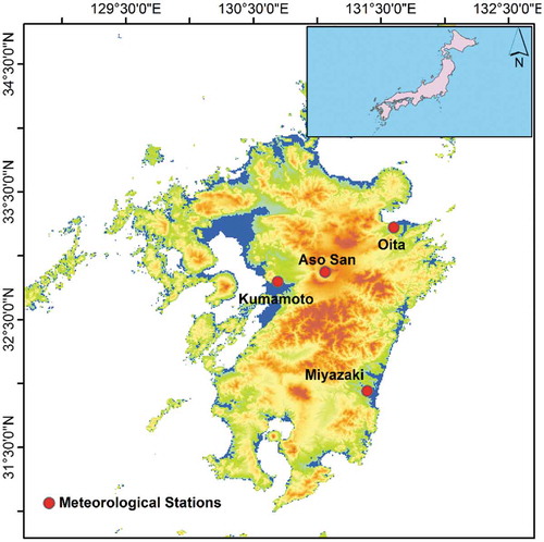
Four meteorological stations (Kumamoto, Aso San, Miyazaki and Oita) located in the southern part of Japan (Fig. 1) were selected as study sites to explore the potential of the proposed model. The study sites enjoy different climate types according to the Köppen-Geiger climate map (Peel et al. 2007). The Kumamoto station falls in humid continental climate (Dfa), Aso san is in humid continental climate (Dfb), whereas Miyazaki and Oita stations are in humid subtropical climate (Cfa). To accomplish this study, monthly meteorological data (Tavg, Tmin, Tmax, Rh, U₂ and Sh) for the period 1980–2017 were collected from the Japan Meteorological Agency (JMA) website.¹ The database contains a few missing values which were filled in with long-term mean values. The general information of all meteorological stations with basic statistical parameters of the climatic variables used for the study period and climate type (Peel et al. 2007) are provided in Table 1.

Table 1. General information of meteorological stations and basic statistical parameters of the meteorological variables for the study period (1980–2017) for four stations located in the southern part of Japan. SD: standard deviation.

Station name	Latitude		Longitude		Altitude (m a.s.l.)	Koppen climate classification
Aso San	32º52.8´N		131º04.4´E		1592	Dfb
Kumamoto	32º 48.8´N		130º 42.4´E		38	Dfa
Miyazaki	31º 52.6´N		131º 26.9´E		6	Cfa
Oita	33º 28.7´N		131º 44.2´E		5	Cfa
	Station: Aso San
	Tavg	Tmin	Tmax	Sh (h)	Wind	Rh	ETo
Statistical parameters	(ºC)	(ºC)	(ºC)	Sh (h)	(km/d)	(%)	(mm/month)
Mean	9.84	6.69	13.5	4.34	397.04	81.59	65.1
SD	7.77	8.09	7.74	1.19	43.32	6.08	27.19
Kurtosis	–1.35	–1.37	–1.26	–0.07	0.39	–0.1	–1.07
Skewness	–0.13	–0.03	–0.21	0.07	0.08	–0.22	0
Minimum	–5.6	–8.6	–2.7	1.2	268	62	18.91
Maximum	22.1	19.3	26.4	8.5	553	96	141.05
	Station: Kumamoto
Mean	16.93	12.48	21.98	5.53	183.55	70.69	93.38
SD	7.87	8.29	7.77	1.25	26.99	5.19	38.95
Kurtosis	–1.36	–1.39	–1.31	–0.31	–0.12	–0.1	–1.11
Skewness	–0.04	0.06	–0.11	0.15	0.33	0.24	0.17
Minimum	2.7	–1.6	7.2	1.8	121	57	35.03
Maximum	29.6	26	35.2	9.3	268	87	181.66
	Station: Miyazaki
Mean	17.62	13.45	22.25	5.85	258.98	73.29	97.07
SD	7.05	7.69	6.53	1.31	36.25	6.47	31.99
Kurtosis	–1.34	–1.37	–1.28	0.16	–0.05	–0.52	–0.55
Skewness	–0.02	0.01	–0.01	–0.22	0.33	–0.29	0.5
Minimum	4.8	–0.2	10.4	1.96	172.8	56	45.36
Maximum	29.8	25.9	34.7	9.73	380.16	90	192.51
	Station: Oita
Mean	16.43	12.48	20.78	5.53	223.03	69.59	93.63
SD	7.4	7.74	7.36	1.23	29.01	6.89	32.56
Kurtosis	–1.34	–1.37	–1.27	0.26	–0.36	–0.69	–0.7
Skewness	0.03	0.09	0.02	0.31	0.04	0.05	0.43
Minimum	3.7	–0.6	7.3	2.43	138.24	53	43.96
Maximum	29.3	25.6	34.6	10.05	293.76	88	185.07

Figure 1. Location of meteorological stations used in this study in Kyushu Islands in the southern part of Japan.

2.2 Empirical estimation of evapotranspiration

The Thornthwaite empirical model (Thornthwaite 1948) was used for estimating ET (ET_T), with monthly Tavg as the main input variable. The Hargreaves method (Hargreaves and Samani 1982, 1985, Hargreaves 1994) was also used for estimating ET (ET_H); this requires monthly Tmin and Tmax data as input variables (Hargreaves 1994). The values of ET_T and ET_H were calculated using the SPEI package (Beguería and Vicente-Serrano 2017) in R programming language.² Reference evapotranspiration (ETo) was calculated by the Penman-Monteith FAO-56 method (Allen et al. 1998) using the CROPWAT 8.0 computer program³ prepared by FAO, with the input variables Tmin, Tmax, Rh, U₂ and Sh. The program estimates extra-terrestrial radiation (Ra) based on the available climatic data and location of the station. A brief discussion of CROPWAT 8.0 is given in Traore et al. (2010). The empirical formulas (Thornthwaite 1948, Hargreaves 1994, Allen et al. 1998) used herein are given in the Supplemental material.

2.3 Support vector regression

Support vector machine (SVM) is a statistical learning theory and the basic algorithm of SVM is put forward by Cortes and Vapnik (1995). SVM is referred to as support vector regression (SVR) when it is applied for solving a regression problem. There are several variations of SVR such as epsilon SVR (ε-SVR), least square SVR (LSSVR) and Nu-SVR (Rahman et al. 2020). In this study, the ε-SVR approach was adopted for modelling since it performs better than the other approaches for ET estimation (Tabari et al. 2012, Raghavendra and Dek 2014, Mehdizadeh et al. 2017, Ferreira et al. 2019). Details regarding ε-SVR are provided in the Supplementary material.

2.4 Prophet model

The Prophet model was introduced by Taylor and Letham (2017). The Prophet model with extra regressor (Taylor and Letham 2017, 2019) has three components: trend, seasonality and regressor with an error term. They can be combined as:

(1)

where the trend function g(t) is used for modelling the non-periodic changes in the time series; s(t) represents the seasonality; and h(t) is an additional regressor. This model is analogous to the generalized additive model (GAM), which has the advantages that it can accommodate new components as required (Taylor and Letham 2017). The trend function g(t) is given as (Taylor and Letham 2017):

(2)

All the parameters related to Equation (2)(2) are discussed below: k denotes the growth rate which is allowed to change by incorporating changepoints over the time period, assuming there are S changepoints at times s_j(j=1,2, …, S). Changes in growth rate that occur at times s_j can be defined by a vector of rate adjustments as . The rate at any time t is equal to the base rate (k) plus all of the adjustments up to that point: This can be presented by a vector as:

(3)

Hence, is the rate at time t.

In Equation (2)(2) , m is an offset parameter which needs adjustment for connecting the endpoints of the segments since k is adjusted. The adjustment at changepoint j can be computed as:

(4)

The seasonality s(t) in Equation (1)(1) is addressed by standard Fourier series (Harvey and Shephard 1993). If P is the regular seasonal period, s(t) can be given as:

(5)

For fittings s(t), it is necessary to estimate 2N parameters . A matrix of seasonality vectors can be generated for estimating parameters at each value of t in the historical time series.

Hence, s(t) can be rewritten as:

(6)

where for seasonality smoothing.

Incorporation of additional regressor h(t) into the model is straightforward by assuming the independent effect of each regressor. This can also be integrated by constructing a matrix of regressors in a similar fashion of seasonality (Taylor and Letham 2017, 2019).

(7)

where z(t) is the matrix of additional regressors and is an extra regressor smoothing parameters.

2.5 Model performance evaluation index

The ETo estimated (for the period 1980–2017) by the Penman-Monteith FAO-56 method was divided into three subsets: training (75%), cross-validation (10%) and test (15%). Previous studies (e.g. Barzegar et al. 2017, Zhang et al. 2018, Mouatadid et al. 2019, Rahman et al. 2020) employed 10–15% data splitting for model validation and testing to avoid over-fitting and generalization ability of the models. The model performance was evaluated by a number of goodness-of-fit (GOF) statistics: coefficient of determination (R²), root mean square error (RMSE), RMSE-observations standard deviation ratio (RSR) (Moriasi et al. 2007), Nash–Sutcliffe efficiency (NSE) (Nash and Sutcliffe 1970) and Kling–Gupta efficiency (KGE) (Gupta et al. 2009).

The coefficient of determination (R²) can be calculated as:

(8)

where y_i, and N indicate observed data, model estimated data and number of data points, respectively.

The NSE can be obtained by (Nash and Sutcliffe 1970):

(9)

The model accuracy can be interpreted based on NSE as very good (0.75 < NSE ≤ 1), good (0.65 < NSE ≤ 0.75), satisfactory (0.50 < NSE ≤ 0.65) and unsatisfactory (NSE ≤ 0.50) (Moriasi et al. 2007).

The root mean square error (RMSE) can be estimated as:

(10)

The RMSE is one of the most useful indexes for performance evaluation (Singh et al. 2004). However, it is difficult to interpret RMSE since there is no recommended value. To overcome the difficulty, Moriasi et al. (2007) developed an RSR index (RMSE-observations standard deviation ratio) which can be used to interpret a model as: very good (0.00 < RSR ≤ 0.50), good (0.50 < RSR ≤ 0.60), satisfactory (0.60 < RSR ≤ 0.70) or (RSR > 0.70) for the monthly time step model (Moriasi et al. 2007).

The RSR is given by:

(11)

where SD_o is the standard deviation of the observed data.

The Kling–Gupta efficiency (KGE) is given by (Gupta et al. 2009):

(12)

where r is the Pearson correlation coefficient; µ_s and µ_o are the mean of observed and model estimated data, respectively; and and are the standard deviation of observed and model estimated data, respectively. The KGE value ranges from – ∞ to 1 and a value closer to 1 indicates accurate model performance. It is more robust than NSE for model performance evaluation since it incorporates several factors such as bias, correlation and a measure of relative variability (Gupta et al. 2009).

3 Model specification

Prophet model with additional regressor (referred to herein as Prophet model) and SVR were used for ETo modelling. In this section, a brief description of the model specification is presented. Focusing first on the Prophet model, it is based on the decomposition of time series data. It allows both additive and multiplicative decomposition approaches. To get the idea about the suitable decomposition approach, we first applied seasonal and trend decomposition using Loess (STL) (Cleveland et al. 1990) to the ETo time series data. We found that additive decomposition is suitable for ETo time series data (see the Supplementary material, Figs. S1 and S2). The Prophet model allows modelling of trend by a piecewise linear model and a saturating growth model (Taylor and Letham 2017). For modelling the trend, we implemented a piecewise linear model since this parsimonious approach is useful for solving regression problems (Taylor and Letham 2017). Several changepoints were placed to accommodate trend changes in the growth of the model and the changepoint range was specified to 0.80 (which means trend changepoints placed within 80% of the training data) to avoid overfitting the model (Taylor and Letham 2017, 2019). Changepoints can be placed manually or automatically; changepoints were selected automatically for this study since it can be done quite naturally using Equation (2)(2) (Taylor and Letham 2017). The other two model parameters, changepoint prior scale and seasonality prior scale, were estimated based on trial and minimization of errors. ET estimation was done when climatic variables (Tavg, Tmin, Tmax, Rh, U₂ and Sh and combinations of these) were used as an additional regressor (Table 2). Regressors were standardized before adding the effect to the trend components (Taylor and Letham 2019). Detailed documentation on model parameter selection and software implementation of the Prophet model is given in Taylor and Letham (2017, 2019).

Table 2. Input variables for Prophet, SVR models and empirical formulas.

Models	Input Variables	Input variables for Empirical formulas
SVR-1 and P-1	Tavg	Thornthwaite method
SVR-2 and P-2	Tmax	-
SVR-3 and P-3	Tmin	-
SVR-4 and P-4	Rh	-
SVR-5 and P-5	U2	-
SVR-6 and P-6	Sh	-
SVR-7 and P-7	Tmin and Tmax	Hargreaves method
SVR-8 and P-8	Tmin, Tmax and Rh	-
SVR-9 and P-9	Tmin, Tmax and Sh	-
SVR-10 and P-10	Tmin, Tmax and U2	-
SVR-11 and P-11	Tmin,Tmax,U2 and Rh	-
SVR-12 and P-12	Tmin,Tmax,U2, Rh and Sh	Penman-Monteith FAO-56 method

With the second model, SVR was also used for estimating ET. The Input combinations of the SVR models were the same as that of Prophet model (Table 2). Data pre-processing using a standardization technique was performed before modelling of ET by SVR to ensure all the variables received enough attention during model training (Sudheer et al. 2003, Wu et al. 2009, Ferreira et al. 2019, Rahman et al. 2020). We executed the SVR modelling in R environment (R Core Development Team 2019) using the “e1071” package (version 1.7–1) (Meyer et al. 2019). There are several kernels for SVR modelling and the most commonly used kernels for hydrological models are linear, radial basis, polynomial and sigmoid (Raghavendra and Dek 2014, Rahman et al. 2020). In this study, the ε-SVR method with a radial basis kernel was adapted for modelling since this combination performs better for ET modelling (Moghaddamnia et al. 2008, Tabari et al. 2012, Mehdizadeh et al. 2017, Ferreira et al. 2019). Beside selection of appropriate kernel function, the performance of SVR models also depends on the values of parameters such as cost (C: regularization parameter), epsilon (ε: width of insensitive tube) and gamma (γ: controls the shape of the hyperplane separation) (Raghavendra and Dek 2014, Suryanarayana et al. 2014, Rahman et al. 2020). However, there is no theory for selecting optimal values for these parameters (Nadiri et al. 2017) and studies generally select these parameters by trial-and-error procedure (Suryanarayana et al. 2014) or based on experience (Zhang et al. 2016). To determine the appropriate parameters for SVR modelling, an efficient automated procedure is required (Zhang et al. 2016, Rahman et al. 2020). In this study, model parameters such as C, ε and γ were determined using the automatic grid search and tune functions of “e1071” R-package. A recent study (Huang et al. 2019) has also successfully obtained model parameters using a grid search function of “e1071” R-package for modelling ET using SVR technique. Details regarding software implementations of the SVR approach are given in Meyer et al. (2019). All the parameters of both models (SVR, Prophet) were finalized using the cross-validation data and no adjustment was made in model parameters during model testing to ensure the generalization capacity of the model.

The input variables for machine learning models (Prophet and SVR) and empirical formulas are provided in Table 2.

4 Results

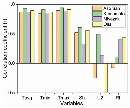
The performance of the models was evaluated by GOF statistics which were calculated by comparing ETo and model estimated ET. The performance statistics of the models with a single input parameter (SVR-1 to SVR-6 and P-1 to P-6) for the test period are given in Table 3. The cross-validation results are given in the Supplementary material (Table S1). The input data of SVR-1 and P-1 models resemble the data required to estimate ET_T. Figure 2 shows the comparisons between ETo and model estimated values in the form of one-to-one plots (left panels) (direct comparisons of GOF are also provided in Table S2). The model (SVR-1 and P-1) estimated values showed closer agreement with those of observed ETo and seasonal patterns were also well captured by both models (Fig. 2, right panels). The temperature-based Thornthwaite method significantly overestimated ETo for summer months and underestimated it for the remaining months (Fig. 2, right panels). Annual variations for the test period (Supplementary material, Fig. S3) showed that annual ET_T was significantly lower than the annual ETo. According to the GOF statistics, the Prophet model (P-1) performed marginally better than the SVR (SVR-1), with average estimated R² values of the four stations being 0.83 (SVR-1) and 0.88 (P-1). Models with Tmax (SVR-2 and P-2) or Tmin (SVR-3 and P-3) as input parameter also showed that the Prophet models gave better accuracy than the SVR models, according to the GOF statistics presented in Table 3. The estimated Pearson correlation coefficient (r) for the test period is shown in Fig. 3 and the correlation coefficient matrix for training, cross-validation and test period are also provided in the Supplementary material (Table S3). It is evident that there is a high correlation (r > 0.80) between ETo and temperature (Tavg, Tmin and Tmax). Furthermore, the SVR models (SVR-4 to SVR-6) with a single input variable of Rh, U₂ or Sh showed unsatisfactory model performance (Moriasi et al. 2007) since the estimated values of NSE and RSR were ≤0.50 and ˃0.70 for all stations, with low values of R² and KGE (Table 3; Supplementary material, Fig. S4). Some studies (Cobaner 2011, Mehdizadeh 2018, Kisi 2018) have also reported unsatisfactory model performance, or higher error for estimating ET using single input variables of Ra, Rh or U₂ by ANN, wavelet ANN, GEP, MARS, ELM and wavelet ELM approaches. On the other hand, Prophet models (P-4 to P-6) with single input of Rh, U₂ or Sh showed very good performance for estimating ET (NSE > 0.75; RSR < 0.50; Supplementary material, Fig. S4) for all four stations. The models incorporating Rh and Sh as an input variable showed almost similar performance compared to the other variables other than temperature data (Table 3). However, the Sh-incorporated model has a good correlation with ETo and showed a low positive correlation (Supplementary material, Table S3). This reveals that there exists a nonlinear relationship between ETo and the mentioned input variables, and machine learning approaches can map the nonlinear relationship between target and input variables and show acceptable performance with limited data (Shiri 2019). The model that incorporated U₂ had the lowest accuracy and showed weak positive or negative correlation with ETo for training, cross-validation and test periods (Supplementary material, Table S3).

Table 3. Comparison between SVR and Prophet model with sole input of climatic variable for the test period.

Station	SVR						Prophet
	Model	RMSE (mm)	RSR	NSE	R^2	KGE	Model	RMSE (mm)	RSR	NSE	R^2	KGE
Aso San	SVR-1	13.26	0.47	0.78	0.79	0.87	P-1	10.83	0.38	0.85	0.88	0.87
	SVR-2	13.51	0.48	0.77	0.78	0.86	P-2	9.09	0.32	0.89	0.91	0.92
	SVR-3	13.92	0.49	0.75	0.76	0.82	P-3	11.66	0.41	0.83	0.87	0.86
	SVR-4	23.98	0.85	0.27	0.29	0.24	P-4	4.9	0.17	0.97	0.97	0.97
	SVR-5	25.77	0.91	0.16	0.20	0.06	P-5	11.67	0.41	0.83	0.88	0.86
	SVR-6	22.56	0.80	0.35	0.38	0.40	P-6	7.22	0.26	0.93	0.97	0.91
Kumamoto	SVR-1	13.86	0.35	0.87	0.88	0.92	P-1	17.62	0.45	0.80	0.92	0.85
	SVR-2	15.96	0.41	0.83	0.85	0.90	P-2	13.93	0.35	0.87	0.94	0.89
	SVR-3	15.96	0.41	0.83	0.85	0.90	P-3	20.17	0.51	0.73	0.91	0.82
	SVR-4	38.70	0.98	0.02	0.03	−0.16	P-4	7.64	0.19	0.96	0.96	0.98
	SVR-5	33.43	0.85	0.27	0.29	0.25	P-5	14.88	0.38	0.85	0.93	0.88
	SVR-6	29.10	0.74	0.45	0.45	0.51	P-6	7.59	0.19	0.96	0.98	0.95
Miyazaki	SVR-1	14.96	0.45	0.79	0.82	0.89	P-1	15.59	0.47	0.78	0.85	0.86
	SVR-2	13.84	0.42	0.82	0.83	0.89	P-2	13.64	0.41	0.83	0.89	0.88
	SVR-3	16.35	0.49	0.75	0.78	0.87	P-3	16.51	0.5	0.75	0.84	0.84
	SVR-4	31.53	0.95	0.08	0.11	0.13	P-4	8.2	0.25	0.94	0.94	0.97
	SVR-5	32.52	0.98	0.02	0.02	−0.19	P-5	12.16	0.37	0.86	0.88	0.87
	SVR-6	28.26	0.85	0.26	0.29	0.24	P-6	8.21	0.25	0.94	0.96	0.92
Oita	SVR-1	14.84	0.43	0.81	0.82	0.89	P-1	14.55	0.42	0.82	0.87	0.85
	SVR-2	13.46	0.39	0.84	0.85	0.90	P-2	12.41	0.36	0.87	0.91	0.89
	SVR-3	17.10	0.50	0.75	0.77	0.87	P-3	16.03	0.47	0.78	0.86	0.83
	SVR-4	32.76	0.95	0.08	0.12	0.20	P-4	8.5	0.25	0.94	0.95	0.95
	SVR-5	30.74	0.89	0.19	0.22	0.24	P-5	15.24	0.44	0.80	0.88	0.86
	SVR-6	25.12	0.73	0.46	0.46	0.52	P-6	7.64	0.22	0.95	0.98	0.91

Figure 2. Comparison of observed and estimated ETo by different models (SVR-1, P-1 and Thornthwaite) with Tavg as input parameters for the test period.

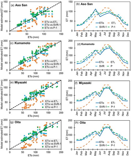
Figure 3. Correlation coefficient between ET_o and climatic variables for the test period.

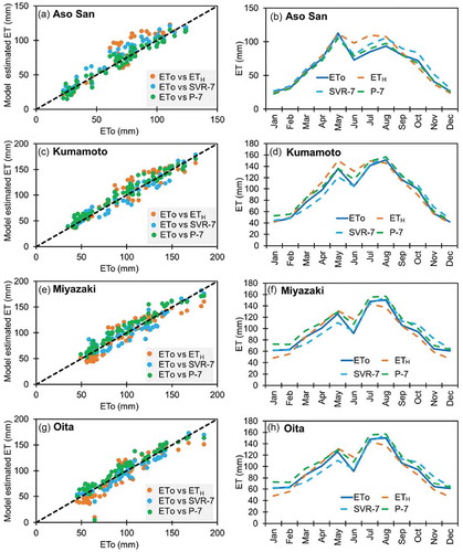
The performance of models with multiple input variables (SVR-7 to SVR-12 and P-7 to P-12) for the test period are given in Table 4. The cross-validation period results are given in the Supplementary material (Table S4). The input data (Tmin and Tmax) of SVR-7 and P-7 models resemble the data required to estimate ET_H. The comparisons between ETo and model-estimated values in the form of one-to-one plot are shown in Fig. 4 (left panels); the seasonal patterns are also shown in Fig. 4 (right panels) and annual comparisons are shown in the Supplementary material (Fig. S5). The model (SVR-7 and P-7) estimated values showed closer agreement with ETo than those estimated by Hargreaves model. The average NSE of the SVR-7 (0.91) and P-7 (0.90) models for the test period were 7% and 6% higher than those (average NSE = 0.84) estimated by Hargreaves model (Supplementary material, Table S5).

Table 4. Comparison between SVR and Prophet model with multiple input of climatic variables for the test period.

Station	SVR						Prophet
	Model	RMSE (mm)	RSR	NSE	R^2	KGE	Model	RMSE (mm)	RSR	NSE	R^2	KGE
Aso San	SVR-7	9.33	0.33	0.89	0.94	0.90	P-7	6.61	0.23	0.94	0.95	0.97
	SVR-8	4.25	0.15	0.98	0.98	0.97	P-8	4.56	0.16	0.97	0.98	0.96
	SVR-9	5.74	0.20	0.96	0.96	0.96	P-9	4.81	0.17	0.97	0.98	0.96
	SVR-10	8.65	0.31	0.90	0.93	0.93	P-10	6.64	0.23	0.94	0.95	0.97
	SVR-11	4.16	0.15	0.98	0.98	0.98	P-11	4.63	0.16	0.97	0.98	0.96
	SVR-12	3.04	0.11	0.99	0.99	0.99	P-12	3.32	0.12	0.99	0.99	0.98
Kumamoto	SVR-7	9.50	0.94	0.94	0.94	0.96	P-7	9.76	0.25	0.94	0.96	0.93
	SVR-8	7.77	0.96	0.96	0.96	0.97	P-8	6.37	0.16	0.97	0.98	0.96
	SVR-9	9.00	0.95	0.95	0.95	0.94	P-9	5.4	0.14	0.98	0.98	0.98
	SVR-10	8.31	0.21	0.95	0.96	0.96	P-10	6.68	0.17	0.97	0.97	0.97
	SVR-11	7.94	0.2	0.96	0.96	0.96	P-11	6.91	0.18	0.97	0.99	0.94
	SVR-12	6.63	0.17	0.97	0.97	0.97	P-12	3.86	0.1	0.99	0.99	0.97
Miyazaki	SVR-7	11.86	0.36	0.87	0.87	0.91	P-7	11.4	0.34	0.88	0.94	0.91
	SVR-8	8.23	0.25	0.94	0.94	0.96	P-8	4.99	0.15	0.98	0.98	0.97
	SVR-9	9.94	0.30	0.91	0.93	0.86	P-9	7.11	0.21	0.95	0.97	0.94
	SVR-10	12.57	0.38	0.85	0.89	0.87	P-10	7.47	0.23	0.95	0.96	0.94
	SVR-11	8.05	0.24	0.94	0.94	0.92	P-11	4.79	0.14	0.98	0.98	0.98
	SVR-12	6.59	0.2	0.96	0.97	0.94	P-12	3.12	0.09	0.99	0.99	0.99
Oita	SVR-7	8.14	0.24	0.94	0.94	0.95	P-7	13.06	0.38	0.85	0.90	0.91
	SVR-8	8.14	0.24	0.94	0.94	0.95	P-8	7.22	0.21	0.96	0.98	0.94
	SVR-9	6.34	0.18	0.97	0.97	0.95	P-9	6.9	0.2	0.96	0.98	0.93
	SVR-10	8.13	0.24	0.94	0.94	0.93	P-10	10.56	0.31	0.90	0.93	0.93
	SVR-11	8.19	0.24	0.94	0.94	0.95	P-11	6.08	0.18	0.97	0.98	0.96
	SVR-12	5.74	0.17	0.97	0.97	0.98	P-12	3.91	0.11	0.99	0.99	0.98

Figure 4. Comparison of observed and estimated ETo by different models (SVR-7, P-7 and Hargreaves) with Tmin and Tmax as input parameters for the test period.

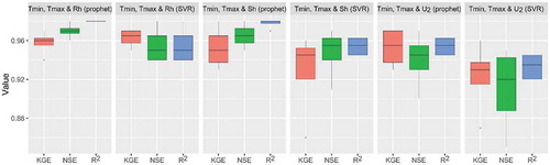
By increasing the input variables (Tmin, Tmax and Rh, U₂ or Sh), the performance of the models was further assessed. Inclusion of Rh or Sh data with Tmin and Tmax was more effective than adding U₂ data (Table 4; Supplementary material, Fig. S6). Figure 5 shows the performance comparison between Prophet (P-8 to P-10) and SVR (SVR-8 to SVR-10) models in terms of NSE, R² and KGE; annual variation is also shown in the Supplementary material (Fig. S6). The expected value of these indicators for the perfect model is unity. The average values of NSE, R² and KGE of the four stations with three models for each station were, respectively, 0.94, 0.95 and 0.94 for SVR models and 0.96, 0.97 and 0.95 for Prophet models.

Figure 5. Comparison of accuracy of models with different input combinations for the test period.

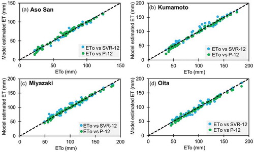
Models with four input variables (SVR-11 and P-11) performed marginally better than models with three input parameters (Table 3, Table 4). ETo estimated by the Prophet model (P-12) with a maximum number of input parameters (Tmin, Tmax, Rh, Sh and U₂) closely followed observed ETo values (Fig. 6) and estimated annual total ETo by the model also showed close agreement with observed (Supplementary material, Fig. S7). The SVR-12 models also showed excellent agreement between model-estimated values and observed ETo. However, comparison of the Prophet models and SVR models in terms of GOF statistics and plots of one-to-one line (Fig. 6) show that the Prophet model-estimated values had closer relationships with the observed ETo. The average values of NSE, RSR, R² and KGE of four stations are, respectively, 0.97, 0.16, 0.98 and 0.97 for the SVR models, and 0.99, 0.11, 0.99 and 0.98 for the Prophet models.

Figure 6. Comparison of observed and estimated ETo by the best models (SVR-12 and P-12) for the test period.

5 Discussion

In this study, the performance of 12 Prophet and SVR models using different combinations of input variables was evaluated and compared, since related literature showed that SVR outperformed the other data-driven approaches (ANN, ANFIS, GEP, MARS and M5 tree) for ETo modelling in different climatic conditions using limited climatic variables (in Iran, USA, Turkey and China) (Tabari et al. 2012, Kisi and Cimen 2009, Kisi 2015, Seifi and Riahi 2018, Huang et al. 2019). ET estimation using limited climatic variables is very important especially for developing countries (e.g., Droogers and Allen 2002, Shiri 2019) where relevant climatic variables such as Rh, Sh and U₂ are not readily available and often unreliable (Droogers and Allen 2002, Almorox et al. 2015). There are a lot of climatic stations that lack a full set of climatic data for ETo estimation even in developed countries (e.g. Japan). On the other hand, good quality temperature data are widely available across the globe (Mendicino and Senatore 2013, Almorox and Grieser 2016). Hence, we investigated the potential of SVR and the Prophet model with limited climatic variables including temperature data as input variables (temperature-based models are P-1, P-2, P-3, P-7 and SVR-1, SVR-2, SVR-3 and SVR-7). As temperature showed higher correlation (r > 0.80) with ETo, the temperature-based model-estimated ET was in close agreement with observed ETo data (Table 3, Table 4). Furthermore, ET estimated with models P-1, P-7, SVR-1 and SVR-7 and those estimated by temperature-based empirical formulas (Thornthwaite and Hargreaves methods) for the test period were also compared with those of observed ETo. The proper local calibration of the Hargreaves method showed improved performance for different climatic regions (Almorox et al. 2015, Feng et al. 2017) except in humid climatic regions (e.g., Nandagiri and Kovoor 2006, Trajkovic 2007, Rahimikhoob 2010, Feng et al. 2017, Chia et al. 2020). Therefore, we did not do any local calibration since the study sites are located in humid climatic regions. Furthermore, a study by Alkaeed et al. (2006) concluded that the Thornthwaite and Hargreaves methods showed good agreement with ETo in the southern part of Japan, while the study compared ETo with ET estimated using several empirical models, such as Thornthwaite (1948), Hargreaves (Hargreaves 1994) and Hamon (Haith and Shoemaker 1987), solar radiation and net radiation-based approaches (Irmak et al. 2003). The findings of this study reveal that the overall accuracy of the machine learning approaches (Prophet and SVR) is generally superior to that of empirical models in estimating ET for the southern part of Japan with limited climatic variables. A number of studies also found that machine learning approaches performed better than standard empirical formulas (e.g., Rahimikhoob 2010, Cobaner 2011, Tabari et al. 2012, Chia et al. 2020) and even locally calibrated formulas (e.g., Rahimikhoob 2010, Shiri 2019, Tikhamarine et al. 2020) for estimating ET with limited climatic variables in different climatic conditions.

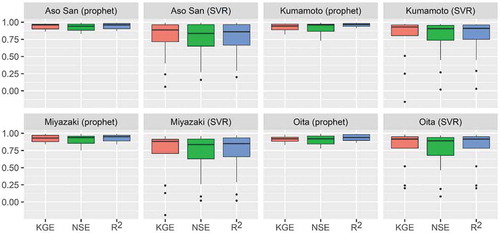
We also compared the accuracy of Prophet (P-1 to P-12) and SVR (SVR-1 to SVR-12) models in terms of NSE, R² and KGE to find out the superior model for the study sites (Fig. 7). The Prophet model is less sensitive to input variables and it can estimate ET with acceptable accuracy using any relevant climatic variables. Hence, the boxplots of the accuracy of the Prophet models (Fig. 7) show that the lower quartile values of these performance indicators are higher than the threshold value (NSE > 0.75) or equivalent to satisfactory model performance value for all stations. However, there are several outliers in the boxplots for SVR models since the model performance was unsatisfactory for several cases (Table 3). In other words, the SVR model is sensitive to temperature data and any relevant variable as input variables other than temperature data cannot estimate ET with acceptable accuracy. The average values of NSE, R² and KGE of four stations with 12 models for each station were, respectively, 0.73, 0.74 and 0.74 for the SVR models and 0.91, 0.94 and 0.92 for the Prophet models. The findings of this study also suggest that model performance generally increased with increasing input variables (Table 3, Table 4). These findings also align with those of a number of other studies (e.g., Seifi and Riahi 2018, Kisi and Alizamir 2018, Huang et al. 2019, Tikhamarine et al. 2020), while these studies also found that machine learning models generally show improved accuracy with increasing number of input variables. The proposed Prophet model with extra regressor tested only in the humid climatic conditions in the southern part of Japan may be applied under other climatic conditions by proper calibration of model parameters. The main advantages of the Prophet model are its simplicity, robustness and speed compared to other machine learning approaches (Aguilera et al. 2019). It is also straightforward to incorporate extra variables/additional regressors even for the non-experts in statistics. The main drawback of this model is the few options for customizing the model parameters (Aguilera et al. 2019, Zhao et al. 2018).

Figure 7. Comparison of accuracy of SVR (SVR-1 to SVR-12) and Prophet (P-1 to P-12) models with 12 different input combinations for the test period.

6 Conclusion

The accuracy of the Prophet model was investigated in modelling monthly reference evapotranspiration using single inputs of the climatic variables temperature, relative humidity, wind speed and sunshine hours and different combinations of these parameters. The obtained results were compared with those of the temperature-based empirical models (Thornthwaite and Hargreaves) and SVR models. The comparative study revealed that temperature-based models (SVR and Prophet) show almost similar accuracy and both performed better than the empirical models for estimating ET. Models with a single input of climatic variables other than temperature data showed that the Prophet model is more flexible than the SVR model in terms of input variables. The accuracy of the models further increased with an increasing number of input parameters and adding Rh or Sh with minimum and maximum temperature can significantly improve the model performance for the southern part of Japan. Models with maximum input parameters also indicated that the Prophet models were superior to the SVR models. Overall, our findings suggest that the Prophet model is generally superior to SVR models with similar data input combinations and less sensitive to input parameters in estimating ET. Further studies in different climatic conditions would help to reveal much about the global implications of the Prophet model for estimating ET using incomplete sets of climatic variables.

Acknowledgements

We sincerely thank the associate editor and anonymous reviewers for their intuitive comments that assisted us to improve the quality of our manuscript significantly. A.T.M.S.R and B.D are grateful to the ministry of culture, sports, science and technology (MEXT) for financial support. A.T.M.S.R is also grateful to all members of hydrology lab, Kumamoto University for their comments and suggestions for improving the quality of this study.

Disclosure statement

Authors have no conflict of interest for publishing this research.

Supplementary material

Supplemental data for this article can be accessed here.

Notes

¹ https://www.data.jma.go.jp/obd/stats/data/en/smp/index.html [Accessed 3 June 2019].

² https://cran.r-project.org/web/packages/SPEI/index.html [Accessed 3 June 2019].

³ http://www.fao.org/land-water/databases-and-software/cropwat/en/ [Accessed 3 June 2019].

References

- Abdullah, S.S., et al., 2015. Extreme learning machines: a new approach for prediction of reference evapotranspiration. Journal of Hydrology, 527, 184–195. doi:10.1016/j.jhydrol.2015.04.073
- Aguilera, H., et al., 2019. Towards flexible groundwater-level prediction for adaptive water management: using Facebook’s Prophet forecasting approach. Hydrological Sciences Journal, 64 (12), 1504–1518. doi:10.1080/02626667.2019.1651933
- Alkaeed, O., et al., 2006. Comparison of several reference evapotranspiration methods for Itoshima Peninsula Area, Fukuoka, Japan. Memoirs of the Faculty of Engineering, Kyushu University, 66 (1), 1–14.
- Allen, R.G., et al. 1998. Crop evapotranspiration guidelines for computing crop water requirements. FAO Irrigation and Drainage, Paper No. 56. Rome: Food and Agriculture Organization of the United Nations.
- Almorox, J. and Grieser, J., 2016. Calibration of the Hargreaves–Samani method for the calculation of reference evapotranspiration in different Koppen climate classes. Hydrology Research, 47 (2), 521–531. doi:10.2166/nh.2015.091
- Almorox, J., Quej, V.H., and Marti, P., 2015. Global performance ranking of temperature-based approaches for evapotranspiration estimation considering Koppen climate classes. Journal of Hydrology, 528, 514–522. doi:10.1016/j.jhydrol.2015.06.057
- Barzegar, R., et al., 2017. Forecasting of groundwater level fluctuations using ensemble hybrid multi-wavelet neural network-based models. Science of Total Environment, 599–600, 20–31. doi:10.1016/j.scitotenv.2017.04.189
- Beguería, S. and Vicente-Serrano, S.M. 2017. Package ‘SPEI’, calculation of the standardised precipitation-evapotranspiration index. [Accessed 1 July 2020]. https://cran.r-project.org/web/packages/SPEI/index.html.
- Castelli, M., et al., 2018. Two-source energy balance modeling of evapotranspiration in Alpine grasslands. Remote Sensing of Environment, 209, 327–342. doi:10.1016/j.rse.2018.02.062
- Chia, M.Y., et al., 2020. Recent advances in evapotranspiration estimation using artificial intelligence approaches with a focus on hybridization techniques—A review. Agronomy, 10, 101. doi:10.3390/agronomy10010101
- Cleveland, R.B., et al., 1990. STL: A seasonal-trend decomposition procedure based on loess. Journal of Official Statistics, 6 (1), 3–73.
- Coats, R.N., 1999. Evaporation, evapotranspiration. In: Environmental geology. Encyclopedia of earth science. Dordrecht: Springer. doi:10.1007/1-4020-4494-1_131
- Cobaner, M., 2011. Evapotranspiration estimation by two different neuro-fuzzy inference systems. Journal of Hydrology, 398 (3–4), 292–302. doi:10.1016/j.jhydrol.2010.12.030
- Colaizzi, P.D., et al., 2012. Two-source energy balance model estimates of evapotranspiration using component and composite surface temperatures. Advances in Water Resources, 50, 134–151. doi:10.1016/j.advwatres.2012.06.004
- Cortes, C. and Vapnik, V., 1995. Support vector networks. Machine Learning, 20, 273–297. doi:10.1007/BF00994018
- Dou, X. and Yang, Y., 2018. Modeling evapotranspiration response to climatic forcings using data-driven techniques in grassland ecosystems. Advances in Meteorology, 1–18. doi:10.1155/2018/1824317
- Droogers, P. and Allen, R.G., 2002. Estimating reference evapotranspiration under inaccurate data conditions. Irrigation and Drainage Systems, 16 (1), 33–45. doi:10.1023/A:1015508322413
- Fan, J., et al., 2018. Evaluation of SVM, ELM and four tree-based ensemble models for predicting daily reference evapotranspiration using limited meteorological data in different climates of China. Agricultural and Forest Meteorology, 263, 225–241. doi:10.1016/j.agrformet.2018.08.019
- Feng, Y., et al., 2016. Comparison of ELM, GANN, WNN and empirical models for estimating reference evapotranspiration in humid region of Southwest China. Journal of Hydrology, 536, 376–383. doi:10.1016/j.jhydrol.2016.02.053
- Feng, Y., et al., 2017. Calibration of Hargreaves model for reference evapotranspiration estimation in Sichuan basin of southwest China. Agricultural Water Management, 181, 1–9. doi:10.1016/j.agwat.2016.11.010
- Ferreira, L.B., et al., 2019. Estimation of reference evapotranspiration in Brazil with limited meteorological data using ANN and SVM–a new approach. Journal of Hydrology, 572, 556–570. doi:10.1016/j.jhydrol.2019.03.028
- Fisher, J.B., et al., 2017. The future of evapotranspiration: global requirements for ecosystem functioning, carbon and climate feedbacks, agricultural management, and water resources. Water Resources Research, 53, 2618–2626. doi:10.1002/2016WR020175
- Gocić, M., et al., 2015. Soft computing approaches for forecasting reference evapotranspiration. Computers and Electronics in Agriculture, 113, 164–173. doi:10.1016/j.compag.2015.02.010
- Gupta, H.V., et al., 2009. Decomposition of the mean squared error and NSE performance criteria: implications for improving hydrological modeling. Journal of Hydrology, 377, 80–91. doi:10.1016/j.jhydrol.2009.08.003
- Haith, D.A. and Shoemaker, L.L., 1987. Generalized watershed loading functions for stream flow nutrients. Water Resources Bulletin, 23, 471–478. doi:10.1111/j.1752-1688.1987.tb00825.x
- Hargreaves, G.H., 1994. Defining and using reference evapotranspiration. Journal of Irrigation and Drainage Engineering, 120 (6), 1132–1139. doi:10.1061/(ASCE)0733-9437(1994)120:6(1132)
- Hargreaves, G.H. and Samani, Z.A., 1982. Estimating potential evapotranspiration. Journal of the Irrigation and Drainage Division, 108 (3), 225–230.
- Hargreaves, G.H. and Samani, Z.A., 1985. Reference crop evapotranspiration from temperature. Applied Engineering in Agriculture, 1, 96–99. doi:10.13031/2013.26773
- Harvey, A.C. and Shephard, N., 1993. Structural time series models. In: G. Maddala, C. Rao, and H. Vinod, eds.. Handbook of statistics. Vol. 11. Amsterdam, Netherlands: Elsevier, 261–302.
- Huang, et al., 2019. Evaluation of CatBoost method for prediction of reference evapotranspiration in humid regions. Journal of Hydrology, 574, 1029–1041. doi:10.1016/j.jhydrol.2019.04.085
- Huntington, T.G., 2010. Climate warming-induced intensification of the hydrological cycle: an assessment of the published record and potential impacts on agriculture. Advances in Agronomy, 109, 1–53.
- Irmak, S., et al., 2003. Solar and net radiation-based equations to estimate reference evapotranspiration in humid climates. Journal of Irrigation and Drainage Engineering, 129 (5), 336–347. doi:10.1061/(ASCE)0733-9437(2003)129:5(336)
- Jones, J.W. and Ritchie, J.T., 1990. Crop growth models. In: G.J. Hoffman, T.A. Howel, and K.H. Solomon, eds. Management of farm irrigation system. ASAE monograph No. 9. St. Joseph, MI: ASAE, 63–89.
- Karimi, S., et al., 2017. Modelling daily reference evapotranspiration in humid locations of South Korea using local and cross-station data management scenarios. International Journal of Climatology, 37, 3238–3246. doi:10.1002/joc.4911
- Kisi, O., 2015. Pan evaporation modeling using least square support vector machine, multivariate adaptive regression splines and M5 model tree. Journal of Hydrology, 528, 312–320. doi:10.1016/j.jhydrol.2015.06.052
- Kisi, O., 2018. Evaporation modelling by heuristic regression approaches using only temperature data. Hydrological Sciences Journal, 64 (4), 653–672. doi:10.1080/02626667.2019.1599487
- Kisi, O. and Alizamir, M., 2018. Modelling reference evapotranspiration using a new wavelet conjunction heuristic method: wavelet extreme learning machine vs wavelet neural networks. Agricultural and Forest Meteorology, 263, 41–48. doi:10.1016/j.agrformet.2018.08.007
- Kisi, O. and Cimen, M., 2009. Evapotranspiration modelling using support vector machines. Hydrological Sciences Journal, 54 (5), 918–928. doi:10.1623/hysj.54.5.918
- Kumar, M., et al., 2008. Comparative study of conventional and artificial neural network based ET0 estimation models. Irrigation Science, 26, 531–545. doi:10.1007/s00271-008-0114-3
- Liu, G., et al., 2012. Comparison of two methods to derive time series of actual evapotranspiration using eddy covariance measurements in the southeastern Australia. Journal of Hydrology, 454–455, 1–6. doi:10.1016/j.jhydrol.2012.05.011
- Malik, A. and Kisi, A., 2017. Monthly pan-evaporation estimation in Indian central Himalayas using different heuristic approaches and climate based models. Computers and Electronics in Agriculture, 143, 302–313. doi:10.1016/j.compag.2017.11.008
- Malik, A. and Kumar, A., 2015. Pan evaporation simulation based on daily meteorological data using soft computing techniques and multiple linear regression. Water Resources Management, 29 (6), 1859–1872. doi:10.1007/s11269-015-0915-0
- Mattar, M.A., 2018. Using gene expression programming in monthly reference evapotranspiration modeling: a case study in Egypt. Agricultural Water Management, 198, 28–38. doi:10.1016/j.agwat.2017.12.017
- Mehdizadeh, S., 2018. Estimation of daily reference evapotranspiration (ETo) using artificial intelligence methods: offering a new approach for lagged ETo data-based modeling. Journal of Hydrology, 559, 794–812. doi:10.1016/j.jhydrol.2018.02.060
- Mehdizadeh, S., Behmanesh, J., and Khalili, K., 2017. Using MARS, SVM, GEP and empirical equations for estimation of monthly mean reference evapotranspiration. Computers and Electronics in Agriculture, 139, 103–114. doi:10.1016/j.compag.2017.05.002
- Mendicino, G. and Senatore, A., 2013. Regionalization of the Hargreaves coefficient for the assessment of distributed reference evapotranspiration in Southern Italy. Journal of Irrigation and Drainage Engineering, 139 (5), 349–362. doi:10.1061/(ASCE)IR.1943-4774.0000547
- Meyer, D., et al., 2019. e1071: misc functions of the department of statistics, probability theory group, TU Wien. Available from https://cran.r-project.org/web/packages/e1071/index.html Accessed 1 Apr 2019.
- Moghaddamnia, A., et al., 2008. Evaporation estimation using sup-port vector machines technique. World Academy of Science, Engineering and Technology, 43, 14–22.
- Moriasi, D.N., et al., 2007. Model evaluation guidelines for systematic quantification of accuracy in watershed simulations. Transactions of the ASABE, 50, 885–900. doi:10.13031/2013.23153
- Mouatadid, S., et al., 2019. Coupling the maximum overlap discrete wavelet transform and long shortterm memory networks for irrigation flow forecasting. Agricultural Water Management, 19, 72–85. doi:10.1016/j.agwat.2019.03.045
- Nadiri, A.A., et al., 2017. Groundwater vulnerability indices conditioned by super-vised intelligence committee machine (SICM). Science of the Total Environment, 574, 691–706. doi:10.1016/j.scitotenv.2016.09.093
- Nandagiri, L. and Kovoor, G.M., 2006. Performance evaluation of reference evapotranspiration equations across a range of Indian climates. Journal of Irrigation and Drainage Engineering, 132 (3), 238–249. doi:10.1061/(ASCE)0733-9437(2006)132:3(238)
- Nash, J.E. and Sutcliffe, J.V., 1970. River flow forecasting through conceptual models part I -a discussion of principles. Journal of Hydrology, 10 (3), 282–290. doi:10.1016/0022-1694(70)90255-6
- Nourani, V., Elkiran, G., and Abdullahi, J., 2019. Multi-station artificial intelligence-based ensemble modeling of reference evapotranspiration using pan evaporation measurements. Journal of Hydrology, 577, 123958. doi:10.1016/j.jhydrol.2019.123958
- Papacharalampous, G., Tyralis, H., and Koutsoyiannis, D., 2018. Predictability of monthly temperature and precipitation using automatic time series forecasting methods. Acta Geophysica, 66, 807–831. doi:10.1007/s11600-018-0120-7
- Peel, M.C., Finlayson, B.L., and McMahon, T.A., 2007. Updated world map of the Köppen-Geiger climate classification. Hydrology and Earth System Sciences, 11, 1633–1644. doi:10.5194/hess-11-1633-2007
- Priestley, C.H.B. and Taylor, R.J., 1972. On the assessment of surface heat flux and evaporation using large scale parameters. Monthly Weather Review, 100, 81–92. doi:10.1175/1520-0493(1972)100<0081:OTAOSH>2.3.CO;2
- Purdy, A.J., et al., 2018. SMAP soil moisture improves global evapotranspiration. Remote Sensing of Environment, 1–14. doi:10.1016/j.rse.2018.09.023
- R Core Development Team, 2019. A language and environment for statistical computing. Vienna, Austria: R Foundation for Statistical Computing.
- Raghavendra, S. and Dek, P.C., 2014. Support vector machine applications in the field of hydrology: a review. Applied Soft Computing, 19, 372–386. doi:10.1016/j.asoc.2014.02.002
- Rahimikhoob, A., 2010. Estimation of evapotranspiration based on only air temperature data using artificial neural networks for a subtropical climate in Iran. Theoretical and Applied Climatology, 101, 83–91. doi:10.1007/s00704-009-0204-z
- Rahman, A.T.M.S., et al., 2018. Modeling the changes in water balance components of the highly irrigated western part of Bangladesh. Hydrology and Earth System Sciences, 22, 4213–4228. doi:10.5194/hess-22-4213-2018
- Rahman, A.T.M.S., et al., 2020. Multiscale groundwater level forecasting: coupling new machine learning approaches with wavelet transforms. Advances in Water Resources, 141, 103595. doi:10.1016/j.advwatres.2020.103595
- Seifi, A. and Riahi, H., 2018. Estimating daily reference evapotranspiration using hybrid gamma test-least square support vector machine, gamma test-ANN, and gamma test-ANFIS models in an arid area of Iran. Journal of Water and Climate Change, jwc2018003. doi:10.2166/wcc.2018.003
- Shiri, J., et al., 2012. Daily reference evapotranspiration modeling by using genetic programming approach in the Basque Country (Northern Spain). Journal of Hydrology, 414–415, 302–316. doi:10.1016/j.jhydrol.2011.11.004
- Shiri, J., 2019. Modeling reference evapotranspiration in island environments: assessing the practical implications. Journal of Hydrology, 570, 265–280. doi:10.1016/j.jhydrol.2018.12.068
- Singh, J., Knapp, H.V., and Demissie, M. 2004. Hydrologic modeling of the Iroquois River watershed using HSPF and SWAT.ISWS CR 2004-08. Champaign, IL: Illinois State Water Survey. Available from https://www.ideals.illinois.edu/handle/2142/94220 Accessed 16 Jun 2019.
- Sudheer, K.P., Nayak, P.C., and Ramasastri, K.S., 2003. Improving peak flow estimates in artificial neural network river flow models. Hydrological Processes, 17, 677–686. doi:10.1002/hyp.5103
- Suryanarayana, C., et al., 2014. An integrated wavelet-support vector machine for groundwater level prediction in Visakhapatnam, India. Neurocomputing, 145, 324–335. doi:10.1016/j.neucom.2014.05.026
- Tabari, H., et al., 2012. SVM, ANFIS, regression and climate-based models for reference evapotranspiration modeling using limited climatic data in a semi-arid highland environment. Journal of Hydrology, 444, 78–89. doi:10.1016/j.jhydrol.2012.04.007
- Taylor, S.J. and Letham, B., 2017. Forecasting at scale. The American Statistician, 72 (1), 37–45. doi:10.1080/00031305.2017.1380080
- Taylor, S.J. and Letham, B. 2019. Prophet: automatic forecasting procedure, R package version 0.5. Available from https://cran.r-project.org/web/packages/Prophet/index.html [Accessed 1 Apr 2019].
- Thornthwaite, C.W., 1948. An approach toward a rational classification of climate. Geographical Review, 38 (1), 55–94. doi:10.2307/210739
- Tikhamarine, Y., et al., 2020. Estimation of monthly reference evapotranspiration using novel hybrid machine learning approaches. Hydrological Sciences Journal. doi:10.1080/02626667.2019.1678750
- Torres, A.F., Walker, W.R., and McKee, M., 2011. Forecasting daily potential evapotranspiration using machine learning and limited climatic data. Agricultural Water Management, 98 (4), 553–562. doi:10.1016/j.agwat.2010.10.012
- Trajkovic, S., 2007. Hargreaves versus Penman-Monteith under humid conditions. Journal of Irrigation and Drainage Engineering, 133 (1), 38–42.
- Traore, S., Wang, Y.M., and Kerh, T., 2010. Artificial neural network for modeling reference evapotranspiration complex process in Sudano-Sahelian zone. Agricultural Water Management, 97, 707–714. doi:10.1016/j.agwat.2010.01.002
- Turc, L., 1961. Evaluation des besoins en eau d’irrigation, evapotranspiration potentielle, formule climatique simplifee et mise a jour. Annales Agronmique, 12 (1), 13–49. ( (in French)).
- Tyralis, H. and Papacharalampous, G.A., 2018. Large-scale assessment of Prophet for multi-step ahead forecasting of monthly streamflow. Advances in Geosciences, 45, 147–153. doi:10.5194/adgeo-45-147-2018
- Wang, L., et al., 2017. Evaporation modelling using different machine learning techniques. International Journal of Climatology, 37, 1076–1092. doi:10.1002/joc.5064
- Wen, X., et al., 2015. Support-vector-machine-based models for modeling daily reference evapotranspiration with limited climatic data in extreme arid regions. Water Resources Management, 29 (9), 3195–3209. doi:10.1007/s11269-015-0990-2
- Wu, C.L., Chau, K.W., and Li, Y.S., 2009. Predicting monthly streamflow using data-driven models coupled with data-preprocessing techniques. Water Resources Research, 45, W08432. doi:10.1029/2007WR006737
- Xu, C.‐.Y., et al., 2006. Analysis of spatial distribution and temporal trend of reference evapotranspiration in Changjiang catchments. Journal of Hydrology, 327, 81–93. doi:10.1016/j.jhydrol.2005.11.029
- Yassin, M.A., Alazba, A.A., and Mattar, M.A., 2016. Artificial neural networks versus gene expression programming for estimating reference evapotranspiration in arid climate. Agricultural Water Management, 163, 110–124. doi:10.1016/j.agwat.2015.09.009
- Zhang, F., et al., 2016. Time series forecasting for building energy consumption using weighted support vector regression with differential evolution, optimization technique. Energy and Buildings, 126, 94–103. doi:10.1016/j.enbuild.2016.05.028
- Zhang, J., et al., 2018. Developing a long short-term memory (LSTM) based model for predicting water table depth in agricultural areas. Journal of Hydrology, 561, 918–929. doi:10.1016/j.jhydrol.2018.04.065
- Zhao, N., et al., 2018. Day-of-week and seasonal patterns of PM2.5 concentrations over the United States: time-series analyses using the Prophet procedure. Atmospheric Environment, 192, 116–127. doi:10.1016/j.atmosenv.2018.08.050