Modification and discussion of the Green-Ampt model for an evolving wetting profile

ABSTRACT

The Green-Ampt (GA) model has been widely used to evaluate soil water infiltration. While a simple piston profile is commonly used, the wetting profile of a soil changes during infiltration and a quarter-ellipse has been found to better describe its evolution. This study aims to improve the GA model and discuss the model parameters when the quarter-ellipse profile is utilized. The soil column is divided into three zones: saturated, transient and dry. The variable γ is introduced to express the ratio of the saturated zone depth to the wetting front depth. A modified GA model is derived via mathematical methods, but an exact solution is difficult to obtain. Therefore, a simplified (SGA) model is developed via a segmented method. Compared with the measured results, the SGA model is more accurate than the traditional model. Finally, the model parameters are discussed and a value of γ = 0.5 is recommended.

KEYWORDS:

• Green-Ampt model
• wetting front depth
• quarter-ellipse profile
• wetting profile

Editor A. Fiori;Associate editor A. Petroselli

1 Introduction

Hydrological models are used to accurately estimate infiltration processes for a wide variety of soil related problems, including the prediction of solute transport, runoff, soil erosion, irrigation, drainage and watershed management (Naderi and Saatsaz 2020). Various infiltration models have been developed for different natural conditions (Al-Janabi et al. 2019). In general, these infiltration models can be classified into semi-empirical, empirical and physically based models (Mishra et al. 2003). The semi-empirical and empirical models use simple expressions but cannot fully describe the infiltration process (Ali et al. 2016). Usually, the parameters in these models are obtained by fitting the infiltration equation to measured data. The physically based models are dependent on the law of conservation of mass and Darcy’s law and their parameters are obtained from the rigorous derivation of equations such as the Richards equation (Richards 1931) and Green-Ampt model (Green and Ampt 1911). The Richards equation simulates infiltration processes more accurately than other methods and is a standard method for the comparison of different models (Hsu et al. 2002). However, an analytical solution is not achievable, except in special cases due to the strong nonlinearity of the equation (Arampatzis et al. 2001). The Green-Ampt (GA) model not only utilizes a simple expression as a semi-empirical and empirical model, but also has the universal applicability of the Richards equation. In addition, the GA model is an attractive alternative when computational time is an issue (Hsu et al. 2002, Liu et al. 2011). Thus, further study of this model is of great significance.

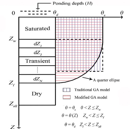
The traditional GA model is based on the assumptions of rectangular saturated piston flow and homogeneous isotropic soil with a uniform initial water content (Barrera and Masuelli 2011, Ali et al. 2016). These assumptions severely limit application of the model; thus, a modified GA model based on them has become a prevalent topic. To date, studies have mainly focused on improving the model for rainfall-runoff simulations and layered soils with nonuniform initial water contents (Corradini et al. 1994, Chu and Mariño 2005, Chen and Young 2006, Rao et al. 2006, Liu et al. 2008, Craig et al. 2010, Ma et al. 2010, Kale and Sahoo 2011, Sajjan et al. 2013, Mohammadzadeh-Habili and Heidarpour 2015, Deng and Zhu 2016, Cui and Zhu 2017). However, a sharp wetting front is always used to describe the infiltration processes, which separates the soil column into wet and dry portions. In this case, the suction head of the dry portion can be considered as a driving force for water infiltration. The driving force is obviously exaggerated compared to the actual situation, where the suction head usually displays a continuous change in the wetting front. To describe the evolving wetting profile better than the simple piston wetting front, Corradini et al. (1997) adopted a similarity curve with a distortable shape that allowed them to analyse infiltration and redistribution during complex rainfall patterns and illustrated that a quarter-ellipse may suitably describe the evolving wetting profile. Wang et al. (2003) tried to improve the GA model using this wetting profile. In their model, the saturated zone depth was always considered to be half of the wetting front depth for loess (i.e. γ = 0.5). The quarter-ellipse, which described the unsaturated zone, was used to calculate the cumulative infiltration (Eq. (20)(20) $I=\left({\theta }_s-{\theta }_d\right)Z_w+0.25\pi \left({\theta }_s-{\theta }_d\right)\left(Z_f-Z_w\right)=\left({\theta }_s-{\theta }_d\right)Z_f\left[\gamma +0.25\pi \left(1-\gamma \right)\right]$(20) ). However, the requirements of the wetting front suction head and hydraulic conductivity were the same as those in the traditional GA model (i.e. the saturated hydraulic conductivity and suction head at the sharp wetting front were adopted). Although Peng et al. (2012) mentioned the variation of γ with the increasing wetting front depth, they did not establish a relationship between the quarter-elliptic wetting profile (transient zone in Fig. 1) and unsaturated hydraulic conductivity. They assumed that the unsaturated hydraulic conductivity had a linear relationship with the depth of the points in the unsaturated region. Furthermore, γ was also considered to change linearly with an increasing wetting front depth. In this work, these assumptions were not adopted. We establish a relationship between the unsaturated hydraulic conductivity and depth of points in the transient zone using the quarter-elliptic equation and extend the relationship between γ and the wetting front depth. These processes are important for the improvement of the GA model.

Figure 1. Schematic diagram of the infiltration model. Z_all is the length of the soil column (cm), and θ(Z) is the water content (cm³/cm³) at depth Z.

There are two main parameters in the GA model, the wetting front suction head and the hydraulic conductivity (Deng and Zhu 2016). Several methods have been suggested for determining the wetting front suction head from the measured soil hydraulic properties (Ma et al. 2010). However, the accuracy of these algorithms must be further verified when considering the evolving wetting profile. The traditional GA model adopted the saturated hydraulic conductivity to simulate the infiltration processes. Bouwer (1966) suggested that the hydraulic conductivity should be half the saturated hydraulic conductivity and Corradini et al. (1997) proposed that the average hydraulic conductivity is more appropriate. The hydraulic conductivity of the infiltration processes is usually regarded as a constant. In other words, the evolving wetting profile has no effect on the hydraulic conductivity. This assumption is clearly different from the actual situation. Therefore, the hydraulic conductivity and wetting front suction head obviously merit further study.

To address the knowledge gap described above, this study aims to: (a) explore the effect of the quarter-elliptic wetting profile on the model parameters (e.g. the hydraulic conductivity and wetting front suction head) and validate the modified GA model presented in this work; and (b) discuss the effect of some parameters, such as the scaling quantity, γ, and the initial water content, θ_d, on the model performance.

2 Materials and methods

2.1 Experimental methods and materials

The experimental results from Ma et al. (2010) and Peng et al. (2012) and the experimental processes are briefly introduced here. The experiments were conducted in a transparent column. The soil materials used in Case 1 were obtained from a soil profile that came from Tuanhe farm in the Daxing District of Beijing, China. Ma et al. (2010) tested a 300-cm-long, five-layered soil column, but only the measured results of the top 100 cm are studied in this work. The subsoil influenced the water infiltration process in the topsoil (Ma et al. 2010, 2011), which led to the recommendation of a factor of 0.8 for the saturated water content by Ma et al. (2010). This factor was adopted in the calculation of the GA model for Case 1. The soil materials used in Case 2 were obtained from Guangyuan, Sichuan Province, China (Peng et al. 2012). These soil samples were air-dried and passed through a sieve before being repacked into a homogeneous soil column. A layer of the soil column was tested by Peng et al. (2012) and their experimental results are discussed in this work.

Determination of the ponding depth was conducted as a constant head by a Mariotte bottle. The cumulative infiltration and infiltration rate were obtained by observing the water table variation of the Mariotte bottle. The wetting front depth was observed to calculate its movement velocity. The physical properties of the soils used are shown in Table 1. For a more detailed experimental setup and instrumentation descriptions, please refer to Ma et al. (2010) and Peng et al. (2012).

Table 1. Physical properties of the soil used in this study according to Ma et al. (2010) and Peng et al. (2012).

Case	Soil depth (cm)	Sand (%)	Silt (%)	Clay (%)	Initial water content, θd (cm^3/cm^3)	Ponding depth, H (cm)
1	100	24.76	59.65	15.59	0.160	7.5
2	85	90.50	8.50	1.00	0.248	15.0

2.2 Traditional GA model

The traditional GA model is a simple description of the infiltration process. According to Darcy’s law, the infiltration rate can be expressed as:

(1) $\frac{\mathrm{d}I}{\mathrm{d}t}=i=k_s\frac{H+S_m+Z_f}{Z_f}$(1)

where I is the cumulative infiltration (cm), i is the infiltration rate (cm/min), k_s is the saturated hydraulic conductivity (cm/min), H is the ponding depth (cm), S_m is the wetting front suction head (cm), Z_f is the wetting front depth (cm) and t is the infiltration time (min).

2.3 Model parameters

The wetting front suction head and hydraulic conductivity are the two main parameters in the GA model (Deng and Zhu 2016). In this study, from top to bottom, soil column is divided into three parts (i.e. the saturated, transient and dry zones, Fig. 1) which more closely aligns with the actual situation (Peng et al. 2012). For the modified GA model, the average hydraulic conductivity is used to replace the saturated hydraulic conductivity of the traditional GA model (Eq. (1)(1) $\frac{\mathrm{d}I}{\mathrm{d}t}=i=k_s\frac{H+S_m+Z_f}{Z_f}$(1) ). The wetting front suction head is achieved by combining the BC model (Brooks and Corey 1966), van Genuchten model (van Genuchten 1980) and Neuman method (Neuman 1976).

2.3.1 Hydraulic conductivity

The evolving wetting profile is described by a rectangle and quarter-ellipse (Fig. 1). The variation in the hydraulic conductivity with the change in unsaturated zone (i.e. transient zone) should be considered. Many models characterize this unsaturated hydraulic conductivity, k_u (Lu and Likos 2004) and the simple and accurate BC model (Brooks and Corey 1966) is adopted in this work. The BC model is expressed as:

(2) $k_u=k_s{S}_e^{\lambda }$(2)

(3) $S_e=\frac{\theta -{\theta }_r}{{\theta }_s-{\theta }_r}$(3)

(4) $\lambda =3+2/\mu$(4)

(5) $\mu =-\frac{\mathrm{d}\left(\mathrm{l}\mathrm{n}{S}_e\right)}{\mathrm{d}\left(\mathrm{l}\mathrm{n}h\right)}$(5)

where S_e is the effective saturation, θ is the water content of the soil (cm³/cm³), θ_r is the residual water content (cm³/cm³), θ_s is the saturated water content (cm³/cm³), μ is the pore-size distribution index, λ is the parameter related to the pore-size distribution index μ, and h is the suction head of the soil (cm).

The relationship between the water content and suction head of the soil is described by the van Genuchten (1980) model, which can be expressed as:

(6) $\begin{array}{cc}\frac{\theta -{\theta }_r}{{\theta }_s-{\theta }_r}={\left(1+{\left|\alpha h\right|}^n\right)}^{-m}& \mathrm{f}\mathrm{o}\mathrm{r}h>0\\ \theta ={\theta }_s& \mathrm{f}\mathrm{o}\mathrm{r}h\le 0\end{array}$(6)

where m, n and α are empirical parameters and m = 1 − 1/n.

Substituting Eq. (6(6) $\begin{array}{cc}\frac{\theta -{\theta }_r}{{\theta }_s-{\theta }_r}={\left(1+{\left|\alpha h\right|}^n\right)}^{-m}& \mathrm{f}\mathrm{o}\mathrm{r}h>0\\ \theta ={\theta }_s& \mathrm{f}\mathrm{o}\mathrm{r}h\le 0\end{array}$(6) ) into Eq. (5(5) $\mu =-\frac{\mathrm{d}\left(\mathrm{l}\mathrm{n}{S}_e\right)}{\mathrm{d}\left(\mathrm{l}\mathrm{n}h\right)}$(5) ), the pore-size distribution index can be written as:

(7) $\mu =\frac{mn{\left(\alpha h\right)}^n}{1+{\left(\alpha h\right)}^n}=mn\left(1-S_e^{1/m}\right)$(7)

To define a single “effective” μ, Lenhard et al. (1989) suggested that the effective saturation, S_e, may be taken as 0.5. Therefore, Eq. (7(7) $\mu =\frac{mn{\left(\alpha h\right)}^n}{1+{\left(\alpha h\right)}^n}=mn\left(1-S_e^{1/m}\right)$(7) ) is written as:

(8) $\mu =mn\left(1-{0.5}_{\hspace{0.17em}}^{1/m}\right)$(8)

The transient zone is divided into numerous segments with the same thickness (i.e. dZ₁ = dZ₂ = … = dZ_N) (Fig. 1). The average hydraulic conductivity of the entire soil layer is obtained and is expressed as:

(9) $\bar{k}=\frac{{\sum }_{j=1}^N\underset{\mathrm{d}{Z}_j\to 0}{lim}{k}_j\mathrm{d}{Z}_j}{Z_f}=\frac{Z_w{k}_s+k_s{\int }_{Z_w}^{Z_f}{\left(\frac{\theta -{\theta }_r}{{\theta }_s-{\theta }_r}\right)}^{\lambda }\mathrm{d}Z}{Z_f}$(9)

(10) $Z_w=\gamma Z_f$(10)

where Z_w is the saturated zone depth (cm), Z is the depth of the points on the wetting profile (cm), k_j is the hydraulic conductivity at the position of the jth segment (cm/min), N is the number of segments and γ is the scaling quantity.

The relationship between the water content, θ, and depth, Z, of the points on the unsaturated wetting profile is described by a quarter-elliptic curve (Corradini et al. 1997, Peng et al. 2012) (Fig. 1), which is expressed as:

(11) ${\left(\frac{\theta -{\theta }_d}{{\theta }_s-{\theta }_d}\right)}^2+{\left(\frac{Z-Z_w}{Z_f-Z_w}\right)}^2=1\left(Z_w\le Z\le Z_f,{\theta }_d\le \theta \le {\theta }_s\right)$(11)

where θ_d is the initial water content (cm³/cm³).

Substituting Eq. (11(11) ${\left(\frac{\theta -{\theta }_d}{{\theta }_s-{\theta }_d}\right)}^2+{\left(\frac{Z-Z_w}{Z_f-Z_w}\right)}^2=1\left(Z_w\le Z\le Z_f,{\theta }_d\le \theta \le {\theta }_s\right)$(11) ) into Eq. (9(9) $\bar{k}=\frac{{\sum }_{j=1}^N\underset{\mathrm{d}{Z}_j\to 0}{lim}{k}_j\mathrm{d}{Z}_j}{Z_f}=\frac{Z_w{k}_s+k_s{\int }_{Z_w}^{Z_f}{\left(\frac{\theta -{\theta }_r}{{\theta }_s-{\theta }_r}\right)}^{\lambda }\mathrm{d}Z}{Z_f}$(9) ), the average hydraulic conductivity can be written as:

(12) $\bar{k}=\gamma k_s+\frac{k_s{\int }_{\gamma Z_f}^{Z_f}{\left(\left({\theta }_s-{\theta }_r\right)\sqrt{1-{\left(\frac{Z-\gamma Z_f}{Z_f-\gamma Z_f}\right)}^2}+{\theta }_d-{\theta }_r\right)}^{\lambda }\mathrm{d}Z}{Z_f{\left({\theta }_s-{\theta }_r\right)}^{\lambda }}$(12)

To simplify Eq. (12(12) $\bar{k}=\gamma k_s+\frac{k_s{\int }_{\gamma Z_f}^{Z_f}{\left(\left({\theta }_s-{\theta }_r\right)\sqrt{1-{\left(\frac{Z-\gamma Z_f}{Z_f-\gamma Z_f}\right)}^2}+{\theta }_d-{\theta }_r\right)}^{\lambda }\mathrm{d}Z}{Z_f{\left({\theta }_s-{\theta }_r\right)}^{\lambda }}$(12) ), the variable X is defined as:

(13) $X=\frac{Z-\gamma Z_f}{Z_f-\gamma Z_f}$(13)

Substituting Eq. (13(13) $X=\frac{Z-\gamma Z_f}{Z_f-\gamma Z_f}$(13) ) into Eq. (12(12) $\bar{k}=\gamma k_s+\frac{k_s{\int }_{\gamma Z_f}^{Z_f}{\left(\left({\theta }_s-{\theta }_r\right)\sqrt{1-{\left(\frac{Z-\gamma Z_f}{Z_f-\gamma Z_f}\right)}^2}+{\theta }_d-{\theta }_r\right)}^{\lambda }\mathrm{d}Z}{Z_f{\left({\theta }_s-{\theta }_r\right)}^{\lambda }}$(12) ), the average hydraulic conductivity can be simplified to:

(14) $\bar{k}=\gamma k_s+\left(1-\gamma \right)k_{s}A$(14)

(15) $A=\frac{{\int }_0^1{\left[\left({\theta }_s-{\theta }_d\right)\sqrt{1-X^2}+{\theta }_d-{\theta }_r\right]}^{\lambda }\mathrm{d}X}{{\left({\theta }_s-{\theta }_r\right)}^{\lambda }}$(15)

In Eq. (14(14) $\bar{k}=\gamma k_s+\left(1-\gamma \right)k_{s}A$(14) ), γk_s represents the effect of the saturated zone’s hydraulic conductivity on the average hydraulic conductivity, whereas (1 − γ)k_sA represents the effect of the transient zone’s hydraulic conductivity on the average hydraulic conductivity.

2.3.2 Wetting front suction head

The effect of the transient zone on the wetting front suction head was considered by Neuman (1976). Hence, this method is used in this study. The wetting front suction head, S_m, is expressed as:

(16) $S_m=\underset{0}{\overset{h_d}{\int }}{k}_r\mathrm{d}h$(16)

(17) $k_r=\frac{k\left(h\right)}{k_s}$(17)

where h is the suction head of the soil (cm), h_d is the initial suction head of the soil (cm), k_r is the relative hydraulic conductivity and k(h) is the unsaturated hydraulic conductivity determined by Eq. (2(2) $k_u=k_s{S}_e^{\lambda }$(2) ).

Combining Eqs. (2(2) $k_u=k_s{S}_e^{\lambda }$(2) )–(8(8) $\mu =mn\left(1-{0.5}_{\hspace{0.17em}}^{1/m}\right)$(8) ) and Eqs. (16)(16) $S_m=\underset{0}{\overset{h_d}{\int }}{k}_r\mathrm{d}h$(16) –(17), S_m can be derived as follows:

(18) $Sm=\underset{0}{\int }{}^{{\frac{\left[{\left(\frac{{\theta }_d-{\theta }_r}{{\theta }_s-{\theta }_r}\right)}^{-1/m}-1\right]}{\alpha }}^{1/n}}{\left(1+{\left|\alpha h\right|}^n\right)}^{-m\lambda }\mathrm{d}h$(18)

2.4 Modified GA model

Through the above analysis, the infiltration rate of the modified GA model can be expressed as:

(19) $i=\bar{k}\frac{H+S_m+Z_f}{Z_f}$(19)

The water balance approach, which is based on the principle of mass conservation, is applied to calculate the cumulative infiltration (i.e. area of the rectangle and quarter-ellipse in Fig. 1):

(20) $I=\left({\theta }_s-{\theta }_d\right)Z_w+0.25\pi \left({\theta }_s-{\theta }_d\right)\left(Z_f-Z_w\right)=\left({\theta }_s-{\theta }_d\right)Z_f\left[\gamma +0.25\pi \left(1-\gamma \right)\right]$(20)

Combining Eqs (14(14) $\bar{k}=\gamma k_s+\left(1-\gamma \right)k_{s}A$(14) ), (19(19) $i=\bar{k}\frac{H+S_m+Z_f}{Z_f}$(19) ) and (20(20) $I=\left({\theta }_s-{\theta }_d\right)Z_w+0.25\pi \left({\theta }_s-{\theta }_d\right)\left(Z_f-Z_w\right)=\left({\theta }_s-{\theta }_d\right)Z_f\left[\gamma +0.25\pi \left(1-\gamma \right)\right]$(20) ), the relationship between the infiltration time and wetting front depth can be expressed as:

(21) $i=\frac{\mathrm{d}I}{\mathrm{d}t}=\left({\theta }_s-{\theta }_d\right)\frac{\mathrm{d}\left\{Z_f\left[\gamma +0.25\pi \left(1-\gamma \right)\right]\right\}}{\mathrm{d}t}=k_s\left[\gamma +\left(1-\gamma \right)A\right]\left(1+\frac{S_m+H}{Z_f}\right)$(21)

(22) $\gamma =g\left(Z_f\right)$(22)

where the relationship between γ and Z_f is expressed by the function g.

Equation (21(21) $i=\frac{\mathrm{d}I}{\mathrm{d}t}=\left({\theta }_s-{\theta }_d\right)\frac{\mathrm{d}\left\{Z_f\left[\gamma +0.25\pi \left(1-\gamma \right)\right]\right\}}{\mathrm{d}t}=k_s\left[\gamma +\left(1-\gamma \right)A\right]\left(1+\frac{S_m+H}{Z_f}\right)$(21) ) seems to be solvable as long as the relationship between γ and Z_f is known and an accurate form of the modified GA model can be obtained (i.e. the AGA model). However, it is often difficult to measure this relationship. In this work, the HYDRUS-1D is adopted as an approximate method to simulate this relationship. The required parameters are shown in Tables 1 and 2.

Table 2. Soil hydraulic parameters according to Ma et al. (2010) and Peng et al. (2012).

Case	θr (cm^3/cm^3)	θs (cm^3/cm^3)	α (1/cm)	n	m	l	ks (cm/min)	λ
1	0.060	0.500	0.0111	1.2968	0.2289	0.5	0.01463	10
2	0.052	0.402	0.012	1.7800	0.428	0.5	0.00780	6

l is the pore-connectivity parameter used in the HYDRUS-1D.

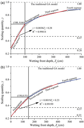
The relationship between γ and Z_f (Eq. (22)(22) $\gamma =g\left(Z_f\right)$(22) ) is shown in Fig. 2. Unfortunately, Eq. (21(21) $i=\frac{\mathrm{d}I}{\mathrm{d}t}=\left({\theta }_s-{\theta }_d\right)\frac{\mathrm{d}\left\{Z_f\left[\gamma +0.25\pi \left(1-\gamma \right)\right]\right\}}{\mathrm{d}t}=k_s\left[\gamma +\left(1-\gamma \right)A\right]\left(1+\frac{S_m+H}{Z_f}\right)$(21) ) remains unsolvable due to the nonlinear relationship between γ and Z_f. Therefore, a segmented method based on calculus is introduced. The curve is divided into finite linear segments and the average γ of each segment is used to calculate the equation (Fig. 2). A simplified form of the modified GA model (i.e. the SGA model) is obtained according to Eq. (21(21) $i=\frac{\mathrm{d}I}{\mathrm{d}t}=\left({\theta }_s-{\theta }_d\right)\frac{\mathrm{d}\left\{Z_f\left[\gamma +0.25\pi \left(1-\gamma \right)\right]\right\}}{\mathrm{d}t}=k_s\left[\gamma +\left(1-\gamma \right)A\right]\left(1+\frac{S_m+H}{Z_f}\right)$(21) ), which can be expressed as:

$t-t_j=\frac{\left({\theta }_s-{\theta }_d\right)\left[{\gamma }_{j+1}+0.25\pi \left(1-{\gamma }_{j+1}\right)\right]}{{\gamma }_{j+1}{k}_s+\left(1-{\gamma }_{j+1}\right)k_{s}A}\times \left[Z_f-Z_{fj}-\left(H+S_m\right)ln\frac{Z_f+H+S_m}{Z_{fj}+H+S_m}\right]$

(23) $Z_{fj}<Z_f\le Z_{f\left(j+1\right)};t_j<t\le t_{j+1};j\in \mathrm{n}\mathrm{a}\mathrm{t}\mathrm{u}\mathrm{r}\mathrm{a}\mathrm{l}\mathrm{n}\mathrm{u}\mathrm{m}\mathrm{b}\mathrm{e}\mathrm{r}$(23)

Figure 2. Relationship between scaling quantity, γ and wetting front depth, Z_f, obtained by HYDRUS-1D: (a) Case 1 and (b) Case 2. R² is the adjusted coefficient of determination.

The initial conditions are:

(24) $Z_{f0}=0;t_0=0$(24)

and the boundary conditions are:

(25) $Z_f=Z_{fj};t=t_j$(25)

where Z_fj and Z_f(j+1) are the minimal and maximal values of the wetting front depth in the (j + 1)th linear segment, respectively (cm); t_j and t_j+1 are the minimal and maximal values of the infiltration time for the (j + 1)th linear segment, respectively (min); and γ_j+1 is the average value of γ in the (j + 1)th linear segment.

The relationship between the wetting front depth and infiltration time is obtained by Eqs. 23(23) $Z_{fj}<Z_f\le Z_{f\left(j+1\right)};t_j<t\le t_{j+1};j\in \mathrm{n}\mathrm{a}\mathrm{t}\mathrm{u}\mathrm{r}\mathrm{a}\mathrm{l}\mathrm{n}\mathrm{u}\mathrm{m}\mathrm{b}\mathrm{e}\mathrm{r}$(23) )–25(25) $Z_f=Z_{fj};t=t_j$(25) ). By substituting the inverse function of Eq. (23(23) $Z_{fj}<Z_f\le Z_{f\left(j+1\right)};t_j<t\le t_{j+1};j\in \mathrm{n}\mathrm{a}\mathrm{t}\mathrm{u}\mathrm{r}\mathrm{a}\mathrm{l}\mathrm{n}\mathrm{u}\mathrm{m}\mathrm{b}\mathrm{e}\mathrm{r}$(23) ) into Eq. (20(20) $I=\left({\theta }_s-{\theta }_d\right)Z_w+0.25\pi \left({\theta }_s-{\theta }_d\right)\left(Z_f-Z_w\right)=\left({\theta }_s-{\theta }_d\right)Z_f\left[\gamma +0.25\pi \left(1-\gamma \right)\right]$(20) ) or Eq. (21(21) $i=\frac{\mathrm{d}I}{\mathrm{d}t}=\left({\theta }_s-{\theta }_d\right)\frac{\mathrm{d}\left\{Z_f\left[\gamma +0.25\pi \left(1-\gamma \right)\right]\right\}}{\mathrm{d}t}=k_s\left[\gamma +\left(1-\gamma \right)A\right]\left(1+\frac{S_m+H}{Z_f}\right)$(21) ), the change in the infiltration rate or cumulative infiltration with an increase in infiltration time can be obtained. Figure 2 shows that calculation of the first segment is generally sufficient to solve most soil–water infiltration problems. Thus, that is the main focus of this work.

2.5 Theoretical basis of HYDRUS-1D

The HYDRUS-1D code is based on the one-dimensional Richards equation to simulate water movement in variably saturated media and uses a finite element numerical approach in space and a finite difference approach in time (Radcliffe and Šimůnek 2010). The water movement equation is given by:

(26) $\frac{\mathrm{\partial }\theta \left(h,t\right)}{\mathrm{\partial }t}=\frac{\mathrm{\partial }}{\mathrm{\partial }{Z}_f}\left[k\left(h\right)\left(\frac{\mathrm{\partial }h}{\mathrm{\partial }{Z}_f}+1\right)\right]$(26)

where θ is the water content of the soil (cm³/cm³), h is the suction head of the soil (cm), t is the infiltration time (min), k(h) is the unsaturated hydraulic conductivity (cm/min) and Z_f is the wetting front depth (cm).

The upper boundary condition assumes constant suction head, which is expressed as:

(27) $h\left(0,t\right)=H$(27)

where H is the ponding depth (cm).

The lower boundary condition assumes the free drainage, which is expressed as:

(28) $\frac{\mathrm{\partial }h}{\mathrm{\partial }{Z}_f}=0$(28)

The initial water content of soil is the same and is expressed as:

(29) $h\left(Z_f,0\right)=h_d$(29)

where h_d is the initial suction head (cm).

2.6 Error estimation and sensitivity analysis

The root mean square error (RMSE) (Zhang et al. 2013), percent bias (PB) (Ali et al. 2016) and Nash-Sutcliffe efficiency coefficient (NSE) (Nash and Sutcliffe 1970) are used to evaluate the error between the traditional GA model, the modified GA model, HYDRUS-1D and the measured results. These metrics are given, respectively, by:

(30) $\mathrm{R}\mathrm{M}\mathrm{S}\mathrm{E}=\sqrt{\frac{{\sum }_{j=1}^N{\left(s_j-o_j\right)}^2}{N}}$(30)

(31) $\mathrm{P}\mathrm{B}=\frac{{\sum }_{j=1}^N\left(s_j-o_j\right)}{{\sum }_{j=1}^N{o}_j}\times 100$(31)

(32) $\mathrm{N}\mathrm{S}\mathrm{E}=1-\frac{{\sum }_{j=1}^N{\left(s_j-o_j\right)}^2}{{\sum }_{j=1}^N{\left(o_j-\bar{o}\right)}^2}=1-{\left(\frac{\mathrm{R}\mathrm{M}\mathrm{S}\mathrm{E}}{\mathrm{S}\mathrm{D}}\right)}^2$(32)

where s_j is the calculated value of the jth sample, o_j is the measured value of the jth sample, ō is the mean of the measured values, N is the number of samples and SD is the standard deviation of the measured values. The RMSE reflects the average absolute error of the calculated and measured values. The PB reflects the relative error of the calculated and measured values. The NSE coefficient reflects the coincidence degree between the calculated and measured values as they vary over time. To quantitatively evaluate the model performance (MP), the criteria presented by Ritter and Muñoz-Carpena (2013) is used: very good (NSE ≥ 0.90, Ⅰ), good (0.80–0.90, Ⅱ), acceptable (0.65–0.80, III) and unsatisfactory (<0.65, Ⅳ).

The sensitivity is expressed by a dimensionless sensitivity index, SI, which is calculated as the ratio between the relative change in the model output and a parameter (Eq. (33)(33) $\mathrm{S}\mathrm{I}=\frac{\frac{y_2-y_1}{y_0}}{\left(\frac{2\mathrm{\Delta }x}{x_0}\right)}$(33) ). A local sensitivity analysis that follows one-at-a-time (OAT) approach is adopted in this work and the procedure is carried out by varying a given parameter according to a given percentage. The base value, x₀, is changed by Δx, which is 20% of x₀ regardless of the potential range of this parameter (i.e. x₀ = x₁ + Δx and x₂ = x₀ + Δx) (Feki et al. 2018). The output results of the corresponding model are y₀, y₁ and y₂, respectively. According to Feki et al. (2018) and Lenhart et al. (2002), the SI was classified as small to negligible (0.00 ≤ |SI| < 0.05), medium (0.05 ≤ |SI| < 0.20), high (0.20 ≤ |SI| < 1.00) and very high (|SI| ≥ 1.00).

The SI is given by:

(33) $\mathrm{S}\mathrm{I}=\frac{\frac{y_2-y_1}{y_0}}{\left(\frac{2\mathrm{\Delta }x}{x_0}\right)}$(33)

3 Results and discussion

3.1 Model validation

3.1.1 Comparison of the SGA and AGA models

The variations in the infiltration characteristics (i.e. the infiltration rate, wetting front depth and cumulative infiltration) with increasing infiltration time are difficult to obtain for the AGA model due to the nonlinear relationship between the scaling quantity, γ and wetting front depth, Z_f (Fig. 2). After simplifying the calculation by using the segmented method, the infiltration characteristics of each segment of the SGA model are shown to have similar expressions to those of the traditional GA model, which are solvable with an increase in the infiltration time, as shown in Eqs. (34)(34) $\frac{\mathrm{d}{Z}_f}{\mathrm{d}t}=\frac{k_s\left[{\gamma }_{j+1}+\left(1-{\gamma }_{j+1}\right)A\right]}{\left({\theta }_s-{\theta }_d\right)\left[{\gamma }_{j+1}+0.25\pi \left(1-{\gamma }_{j+1}\right)\right]}\left(1+\frac{S_m+H}{Z_f}\right)$(34) –(35(35) $\frac{\mathrm{d}{Z}_f}{\mathrm{d}t}=\frac{k_s}{\left({\theta }_s-{\theta }_d\right)}\left(1+\frac{S_m+H}{Z_f}\right)$(35) ). Therefore, the SGA model can be considered in place of the AGA model, but the accuracy of the SGA model must be validated.

The SGA model:

(34) $\frac{\mathrm{d}{Z}_f}{\mathrm{d}t}=\frac{k_s\left[{\gamma }_{j+1}+\left(1-{\gamma }_{j+1}\right)A\right]}{\left({\theta }_s-{\theta }_d\right)\left[{\gamma }_{j+1}+0.25\pi \left(1-{\gamma }_{j+1}\right)\right]}\left(1+\frac{S_m+H}{Z_f}\right)$(34)

The traditional GA model:

(35) $\frac{\mathrm{d}{Z}_f}{\mathrm{d}t}=\frac{k_s}{\left({\theta }_s-{\theta }_d\right)}\left(1+\frac{S_m+H}{Z_f}\right)$(35)

In Case 2, the changes in the wetting front depth and cumulative infiltration with an increase in the infiltration time were obtained by Peng et al. (2012), while the relationship between the infiltration rate and infiltration time was not measured. An approximate method is often used to calculate the measured infiltration rate when the variation in the infiltration time (Δt) is sufficiently small, as shown in Eq. (36)(36) $i=\frac{\mathrm{\Delta }\mathrm{I}}{\mathrm{\Delta }\mathrm{t}}$(36) . Peng et al. (2012) measured the cumulative infiltration about once an hour and this large time interval may have resulted in obvious deviations in the infiltration rate, especially during the early infiltration stage. Consequently, the measured results of the infiltration rate for Case 2 are not given in this work.

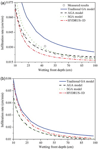
Figure 3 shows a comparison between the infiltration rate according to Eq. (36)(36) $i=\frac{\mathrm{\Delta }\mathrm{I}}{\mathrm{\Delta }\mathrm{t}}$(36) and the wetting front depth for the SGA and AGA models. The infiltration simulated by the AGA model provided the best agreement with the measured results and the calculated results of the SGA model were very close to the AGA model. Therefore, the SGA model may be used to accurately predict infiltration instead of the complex AGA model.

(36) $i=\frac{\mathrm{\Delta }\mathrm{I}}{\mathrm{\Delta }\mathrm{t}}$(36)

Figure 3. Relationship between infiltration rate, i and wetting front depth, Z_f, as simulated by the traditional GA model, the AGA model, the SGA model and HYDRUS-1D: (a) Case 1 and (b) Case 2. Measured results according to Ma et al. (2010) and Peng et al. (2012).

where ΔI denotes the variation in the cumulative infiltration during the variational time, Δt.

3.1.2 Comparison of the SGA model with the traditional GA model, HYDRUS-1D and measured results

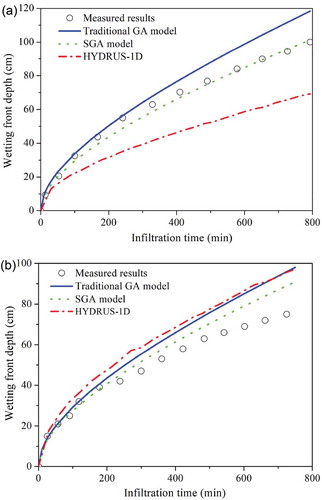
Figure 4 shows a comparison of the wetting front depth predicted by the traditional GA model, SGA model and HYDRUS-1D. The wetting front depth increases with increasing infiltration time. During the early infiltration stage, the increase is rapid and then gradually slows down until the velocity of the infiltration (dZ_f/dt) ultimately approximates a constant. Comparing the results of these three models reveals that the traditional GA model and SGA model both produce results that are close to the measured results during the early stage of infiltration. However, the traditional GA model gradually deviates from the measured results as the infiltration time continues to increase. The results produced by the HYDRUS-1D in Case 2 are slightly higher than those of the other two models but are significantly lower than the measured results in Case 1, as evidenced in Fig. 4 and Table 3.

Table 3. Error estimation showing the model performance (MP). RMSE: root mean square error; PB: percent bias; NSE: Nash-Sutcliffe efficiency coefficient.

Case	Category	Traditional GA model				Modified GA model				HYDRUS-1D
		RMSE	PB (%)	NSE	MP	RMSE	PB (%)	NSE	MP	RMSE	PB (%)	NSE	MP
1	Wetting front depth	9.597	12.8	0.910	Ⅰ	2.765	−2.8	0.993	Ⅰ	20.838	−31.4	0.576	Ⅳ
	Infiltration rate	0.009	33.8	−0.679	Ⅳ	0.002	4.6	0.884	Ⅱ	0.002	1.4	0.952	Ⅰ
	Cumulative infiltration	3.196	25.6	0.728	III	0.673	−5.0	0.988	Ⅰ	0.731	−5.4	0.986	Ⅰ
2	Wetting front depth	10.546	17.6	0.772	III	6.524	9.4	0.913	Ⅰ	10.808	20.5	0.761	III
	Cumulative infiltration	1.166	12.2	0.894	Ⅱ	0.635	−7.4	0.968	Ⅰ	0.635	−7.0	0.969	Ⅰ

Figure 4. Comparison of the wetting front depth calculated by the traditional GA model, the SGA model and HYDRUS-1D: (a) Case 1 and (b) Case 2. Measured results according to Ma et al. (2010) and Peng et al. (2012).

Figure 5 shows that the infiltration rate decreases with an increase in infiltration time and the cumulative infiltration increases with an increase in infiltration time. The infiltration rate and cumulative infiltration simulated by the SGA model and HYDRUS-1D are basically consistent and they approach the measured results. However, the results of the traditional GA model are somewhat larger than the measured results, especially in the later stage of infiltration, as evidenced in Fig. 5 and Table 3.

Figure 5. Comparisons of the infiltration rate and cumulative infiltration simulated by the traditional GA model, the SGA model and HYDRUS-1D: (a) Case 1 and (b) Case 2. Measured results according to Ma et al. (2010) and Peng et al. (2012).

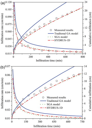
According to Ritter and Muñoz-Carpena (2013), Table 3 shows that the MP of the SGA model is very good or good; the traditional GA model has poor performance in the infiltration rate, while the performance of other infiltration characteristics are satisfactory (including acceptable, good and very good); and the HYDRUS-1D produces unsatisfactory results for the wetting front depth in Case 1, whereas its performances for the infiltration rate and cumulative infiltration are very good. Overall, the SGA model describes the infiltration process better than the other two models in this work.

In Case 1, the experiment on the five-layered soil column was performed by Ma et al. (2010). Although only the measured results from the top 100 cm of the soil column are studied in this work, the influence of the subsoil on the topsoil still needs attention. Ma et al. (2010, 2011) illustrated that the results of the wetting front depth calculated by the HYDRUS-1D were significantly lower than the measured results due to entrapped air bubbles left in the soil pores, which caused the actual hydraulic conductivity of the saturated zone to be lower than the saturated hydraulic conductivity that was predicted by the RETC code. In Case 2 (a layer of the soil column), the results of the wetting front depth calculated by the HYDRUS-1D were more accurate than those of Case 1. As a result of a comprehensive analysis of these two cases, it was determined that layered soil increased the entrapped air bubbles left in the soil pores, which caused significant deviations from the hydraulic conductivity. Therefore, selection of the infiltration parameter should be carefully considered for layered soil.

For the one-dimensional soil column infiltration studied in this work, the wetting front depth, infiltration rate and cumulative infiltration are calculated by the traditional GA model, SGA model and HYDRUS-1D. The infiltration characteristics are exaggerated by the traditional GA model without considering the evolving wetting profile, the HYDRUS-1D, with suitable parameters, is accurate, especially in terms of the infiltration rate and cumulative infiltration and the SGA model describes the infiltration process the best. The wetting front suction head as presented by Neuman is still applicable when considering the evolving wetting profile.

3.2 Influence of the scaling quantity, γ and initial water content, θ_d, on the model

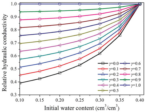
The initial water content, θ_d and scaling quantity, γ, are different from other hydraulic parameters determined by grain composition and soil density. Brakensiek and Onstad (1977) found that the error caused by the hydraulic conductivity, k and (θ_s − θ_d) was greater than the suction head. Equations (14) and (15) show that the average hydraulic conductivity can be affected by the initial water content, θ_d and a scaling quantity, γ. Therefore, the effects of parameters θ_d and γ on the relative hydraulic conductivity, k_r and wetting front depth, Z_f, are further discussed.

Figure 6 shows that the relative hydraulic conductivity increases with an increase in γ for a given initial water content. When the initial water content approaches the saturated water content, the variation in γ has little effect on the relative hydraulic conductivity. For a given γ, the relative hydraulic conductivity increases with increasing initial water content. When γ approaches one, the effect of the initial water content on the relative hydraulic conductivity may be ignored. The traditional GA model is a special case in which γ is equal to one (Fig. 2) and the results it produces may indicate a noticeable deviation from the actual situation when dry soils are studied.

Figure 6. Relationship between the relative hydraulic conductivity and initial water content.

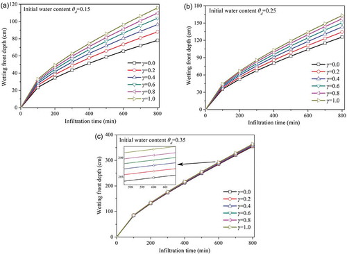
Figure 7 shows that, for a given infiltration time, the wetting front depth increases as γ increases. During the early infiltration stage, γ has little effect on the wetting front depth. Therefore, the wetting front depth determined by the traditional GA model (γ = 1) is close to that from the SGA model for the first 200 min (Fig. 4). However, as the infiltration time continues to increase, the influence of γ gradually becomes significant, which is the reason why these two models differ significantly in the later stage of infiltration. The higher the initial water content, the faster the wetting front depth changes with the increase in infiltration time. When the initial water content is close to the residual water content, γ has a significant effect on the wetting front depth. However, when the soil column approaches the saturated state, the influence of γ on the wetting front depth can be ignored. The traditional GA model should be applied to soils with a high initial water content. When the relationship between γ and Z_f cannot be obtained, a median value of γ = 0.5 is recommended for predicting the infiltration characteristics. This value was shown to be suitable for the prediction of water infiltration in loess by Wang et al. (2003). This study confirms this finding and believes that its scope of application is wider than only loess. Lu and Likos (2004) illustrated that the applicability of the BC model and approximation of the hydraulic conductivity is generally limited to relatively coarse-grained soil. The BC model used in this study limits the application scope of the modified GA model, i.e. the SGA model is also suitable for relatively coarse-grained soil. According to the results of this work, the soils used in Case 1 and Case 2 can be considered as relatively coarse-grained soil in the modified model.

Figure 7. Relationship between the wetting front depth and infiltration time: (a) initial water content θ_d = 0.15, (b) initial water content θ_d = 0.25 and (c) initial water content θ_d = 0.35.

3.3 Influence of the pore-size distribution index, μ and effective saturation, S_e (Eq. (7)(7) $\mu =\frac{mn{\left(\alpha h\right)}^n}{1+{\left(\alpha h\right)}^n}=mn\left(1-S_e^{1/m}\right)$(7) ) on the model

The approximate algorithm for μ is presented in Eq. (8)(8) $\mu =mn\left(1-{0.5}_{\hspace{0.17em}}^{1/m}\right)$(8) . The value of μ in Case 1 is 0.28 and that in Case 2 is 0.61. Thus, μ values of 0.25, 0.35, 0.45, 0.55 and 0.65 are analysed to determine its effect on the infiltration characteristics. The other soil parameters are taken from Case 1. Figure 8 shows that the wetting front depth, cumulative infiltration and infiltration rate increase with increasing μ values. As the infiltration time increases, the influence of μ on the wetting front depth and cumulative infiltration gradually becomes significant, whereas its effect on the infiltration rate becomes weak. When the infiltration time is 800 min, an increase in μ from 0.25 to 0.65 increases the wetting front depth from 97 cm to 137 cm, the infiltration rate from 0.017 cm/min to 0.023 cm/min and the cumulative infiltration from 21 cm to 30 cm. The μ with a wide range of values has a non-negligible impact on the results of the model. In fact, the range of μ values is determined by the effective saturation, S_e (Eq. (7(7) $\mu =\frac{mn{\left(\alpha h\right)}^n}{1+{\left(\alpha h\right)}^n}=mn\left(1-S_e^{1/m}\right)$(7) )(7) $\mu =\frac{mn{\left(\alpha h\right)}^n}{1+{\left(\alpha h\right)}^n}=mn\left(1-S_e^{1/m}\right)$(7) ). In this work, S_e is approximately 0.5, as recommended by Lenhard et al. (1989). The sensitivity of the parameter, S_e, to the model determines whether the approximate algorithm is reasonable. S_e = 0.5 is used in this study as the base value of x₀ and the sensitivity of the infiltration characteristics output to input parameter, S_e (Eq. 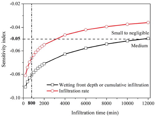(7(7) $\mu =\frac{mn{\left(\alpha h\right)}^n}{1+{\left(\alpha h\right)}^n}=mn\left(1-S_e^{1/m}\right)$(7) )) is shown in Fig. 9. As the infiltration time increases, the SI of the infiltration characteristics decreases. According to Feki et al. (2018) and Lenhart et al. (2002), these sensitivity indexes are classified as medium (0.05 ≤ |SI| < 0.20) at 800 min. The SI of the infiltration rate is classified as small to negligible (0.00 ≤ |SI| < 0.05) when the infiltration time exceeds 3158 min, whereas the small to negligible sensitivity of the wetting front depth and cumulative infiltration occurs at 11472 min. The sensitivity of the infiltration characteristics output to input parameter, S_e (Eq. (7(7) $\mu =\frac{mn{\left(\alpha h\right)}^n}{1+{\left(\alpha h\right)}^n}=mn\left(1-S_e^{1/m}\right)$(7) )) is not high. Specifically, an increase in S_e from 0.4 to 0.6 (0.5 ± 0.1) decreases μ from 0.29 to 0.27 and this variation of μ has little effect on the MP according to Fig. 8. Overall, the approximate algorithm of Eq. (8)(8) $\mu =mn\left(1-{0.5}_{\hspace{0.17em}}^{1/m}\right)$(8) is considered to be suitable for this study.

Figure 8. Impact of μ on the infiltration characteristics: (a) wetting front depth, (b) infiltration rate and (c) cumulative infiltration.

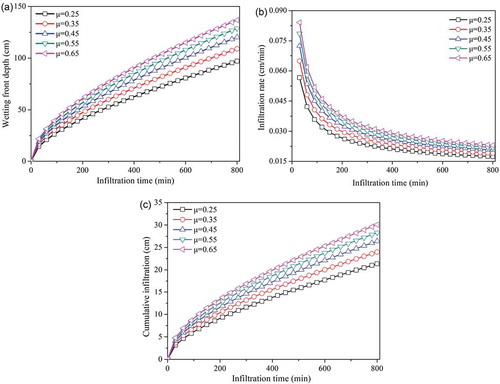
Figure 9. Sensitivity of the infiltration characteristics output to input parameter, S_e (Eq. (7)(7) $\mu =\frac{mn{\left(\alpha h\right)}^n}{1+{\left(\alpha h\right)}^n}=mn\left(1-S_e^{1/m}\right)$(7) ).

3.4 Application of the model to a rainfall–runoff simulation

The traditional GA model was applied to a rainfall-runoff simulation by Mein and Larson (1973) and they illustrated three different cases of infiltration for the rainfall. The model presented in this work has the potential to improve the accuracy of the rainfall-runoff simulation compared to the traditional GA model. It can more accurately describe the water content distribution owing to the quarter-ellipse and the average hydraulic conductivity calculated by this work is significantly better than the saturated hydraulic conductivity when the topsoil is not saturated (i.e. the maximum water content is less than the saturated water content at this time). Furthermore, this model has the potential to describe the redistribution of the water content after a rainfall using the water balance approach, which is similar to the idea proposed by Corradini et al. (1997). This model may also be used for slope stability analyses under rainfall conditions and water infiltration analyses in layered soils. Of course, some assumptions are necessary when this model is applied in these areas and should be further studied in the future.

4 Conclusion

In this study, we develop a modified GA model with a quarter-ellipse wetting front to simulate the infiltration process. The scaling quantity, γ, i.e. the ratio of the saturated zone depth to the wetting front depth, is an important parameter in the model and the variation in the average hydraulic conductivity with the wetting profile is described by this parameter. The results of the traditional GA model, HYDRUS-1D (i.e. the Richards equation) and experiments in the literature are explored to compare and validate the SGA model. The RMSE, PB and NSE are used as indicators to evaluate the MP.

The results showed that the performance of the SGA model is optimal or near-optimal; the HYDRUS-1D produces unsatisfactory results for the wetting front depth in Case 1 due to the neglect of entrapped air bubbles left in the soil pores, whereas the performance for the infiltration rate and cumulative infiltration are very good; and the performance of the traditional GA model is poorer than that of the SGA model owing to the use of a sharpened piston profile (i.e. neglecting the changes in the evolving wetting profile). Therefore, the proposed SGA model reasonably describes the infiltration process.

Some important parameters are also discussed in this work. When the initial water content approaches the residual water content, the influence of γ on the relative hydraulic conductivity is remarkable. However, as the initial water content increases, this influence becomes increasingly small. A value of γ = 0.5 is recommended to predict the infiltration process, instead of the traditional GA model’s recommendation of γ = 1. The sensitivity of the infiltration characteristics output to input parameter, S_e, in Eq. (7)(7) $\mu =\frac{mn{\left(\alpha h\right)}^n}{1+{\left(\alpha h\right)}^n}=mn\left(1-S_e^{1/m}\right)$(7) is medium and small to negligible and the approximate algorithm shown in Eq. (8)(8) $\mu =mn\left(1-{0.5}_{\hspace{0.17em}}^{1/m}\right)$(8) is suitable for this study. The SGA model is more suitable for relatively coarse-grained soils due to the BC model used in this study.

Acknowledgements

The authors are thankful to the editors and anonymous reviewers for their valuable suggestions and comments which helped to improve the manuscript.

Disclosure statement

No potential conflict of interest was reported by the authors.

Additional information

Funding

This work was supported by National Natural Science Foundation of China [no. 51578272].

References

- Ali, S., et al., 2016. Green-Ampt approximations: a comprehensive analysis. Journal of Hydrology, 535, 340–355. doi:10.1016/j.jhydrol.2016.01.065
- Al-Janabi, A.M.S., Ghazali, A.H., and Yusuf, B., 2019. Modified models for better prediction of infiltration rates in trapezoidal permeable stormwater channels. Hydrological Sciences Journal, 64 (15), 1918–1931. doi:10.1080/02626667.2019.1680845
- Arampatzis, G., et al., 2001. Estimation of unsaturated flow in layered soils with the finite control volume method. Irrigation and Drainage, 50 (4), 349–358. doi:10.1002/ird.31
- Barrera, D. and Masuelli, S., 2011. An extension of the Green-Ampt model to decreasing flooding depth conditions, with efficient dimensionless parametric solution. Hydrological Sciences Journal, 56 (5), 824–833. doi:10.1080/02626667.2011.585137
- Bouwer, H., 1966. Rapid field measurement of air entry value and hydraulic conductivity of soil as significant parameters in flow system analysis. Water Resources Research, 2 (4), 729–738. doi:10.1029/WR002i004p00729
- Brakensiek, D.L. and Onstad, C.A., 1977. Parameter estimation of the Green and Ampt infiltration equation. Water Resources Research, 13 (6), 1009–1012. doi:10.1029/WR013i006p01009
- Brooks, R.H. and Corey, A.T., 1966. Properties of porous media affecting fluid flow. Journal of the Irrigation and Drainage Division, 92 (2), 61–88.
- Chen, L. and Young, M.H., 2006. Green-Ampt infiltration model for sloping surfaces. Water Resources Research, 42 (7), W07420. doi:10.1029/2005wr004468
- Chu, X.F. and Mariño, M.A., 2005. Determination of ponding condition and infiltration into layered soils under unsteady rainfall. Journal of Hydrology, 313 (3–4), 195–207. doi:10.1016/j.jhydrol.2005.03.002
- Corradini, C., Melone, F., and Smith, R.E., 1994. Modeling infiltration during complex rainfall sequences. Water Resources Research, 30 (10), 2777–2784. doi:10.1029/94WR00951
- Corradini, C., Melone, F., and Smith, R.E., 1997. A unified model for infiltration and redistribution during complex rainfall patterns. Journal of Hydrology, 192 (1–4), 104–124. doi:10.1016/s0022-1694(96)03110-1
- Craig, J.R., Liu, G., and Soulis, E.D., 2010. Runoff-infiltration partitioning using an upscaled Green-Ampt solution. Hydrological Processes, 24 (16), 2328–2334. doi:10.1002/hyp.7601
- Cui, G.T. and Zhu, J.T., 2017. Infiltration model in sloping layered soils and guidelines for model parameter estimation. Hydrological Sciences Journal, 62 (13), 2222–2237. doi:10.1080/02626667.2017.1371848
- Deng, P. and Zhu, J.T., 2016. Analysis of effective Green-Ampt hydraulic parameters for vertically layered soils. Journal of Hydrology, 538, 705–712. doi:10.1016/j.jhydrol.2016.04.059
- Feki, M., et al., 2018. Impact of infiltration process modeling on soil water content simulations for irrigation management. Water, 10 (7), 850. doi:10.3390/w10070850
- Green, W.H. and Ampt, G.A., 1911. Study on soil physics: I. Flow of air and water through soils. Journal of Agricultural Science, 4, 1–24.
- Hsu, S.M., Ni, C.F., and Hung, P.F., 2002. Assessment of three infiltration formulas based on model fitting on Richards equation. Journal of Hydrologic Engineering, 7 (5), 373–379. doi:10.1061/(ASCE)1084-0699(2002)7:5(373)
- Kale, R.V. and Sahoo, B., 2011. Green-Ampt infiltration models for varied field conditions: a revisit. Water Resources Management, 25 (14), 3505–3536. doi:10.1007/s11269-011-9868-0
- Lenhard, R.J., Parker, J.C., and Mishra, S., 1989. On the correspondence between Brooks-Corey and van Genuchten models. Journal of Irrigation and Drainage Engineering, 115 (4), 744–751. doi:10.1061/(ASCE)0733-9437(1989)115:4(744)
- Lenhart, T., et al., 2002. Comparison of two different approaches of sensitivity analysis. Physics and Chemistry of the Earth, 27 (9–10), 645–654. doi:10.1016/s1474-7065(02)00049-9
- Liu, G., Craig, J.R., and Soulis, E.D., 2011. Applicability of the Green-Ampt infiltration model with shallow boundary conditions. Journal of Hydrologic Engineering, 16 (3), 266–273. doi:10.1061/(ASCE)HE.1943-5584.0000308
- Liu, J.T., Zhang, J.B., and Feng, J., 2008. Green-Ampt model for layered soils with nonuniform initial water content under unsteady infiltration. Soil Science Society of America Journal, 72 (4), 1041–1047. doi:10.2136/sssaj2007.0119
- Lu, N. and Likos, W.J., 2004. Unsaturated soil mechanics. Hoboken: John Wiley & Sons.
- Ma, Y., et al., 2010. Modeling water infiltration in a large layered soil column with a modified Green-Ampt model and HYDRUS-1D. Computers and Electronics in Agriculture, 71 (1), S40–S47. doi:10.1016/j.compag.2009.07.006
- Ma, Y., et al., 2011. Water infiltration in layered soils with air entrapment: modified Green-Ampt model and experimental validation. Journal of Hydrologic Engineering, 16 (8), 628–638. doi:10.1061/(ASCE)HE.1943-5584.0000360
- Mein, R.G. and Larson, C.L., 1973. Modeling infiltration during a steady rain. Water Resources Research, 9 (2), 384–394. doi:10.1029/wr009i002p00384
- Mishra, S.K., Tyagi, J.V., and Singh, V.P., 2003. Comparison of infiltration models. Hydrological Processes, 17 (13), 2629–2652. doi:10.1002/hyp.1257
- Mohammadzadeh-Habili, J. and Heidarpour, M., 2015. Application of the Green-Ampt model for infiltration into layered soils. Journal of Hydrology, 527, 824–832. doi:10.1016/j.jhydrol.2015.05.052
- Naderi, M. and Saatsaz, M., 2020. Impact of climate change on the hydrology and water salinity in the Anzali Wetland, northern Iran. Hydrological Sciences Journal, 65 (4), 552–570. doi:10.1080/02626667.2019.1704761
- Nash, J.E. and Sutcliffe, J.V., 1970. River flow forecasting through conceptual models part I-A discussion of principles. Journal of Hydrology, 10 (3), 282–290. doi:10.1016/0022-1694(70)90255-6
- Neuman, S.P., 1976. Wetting front pressure head in the infiltration model of Green and Ampt. Water Resources Research, 12 (3), 564–566. doi:10.1029/WR012i003p00564
- Peng, Z.Y., et al., 2012. Modification of Green-Ampt model based on the stratification hypothesis. [ In Chinese] Advances in Water Science, 23 (1), 59–66.
- Radcliffe, D.E. and Šimůnek, J., 2010. Soil physics with HYDRUS: modeling and applications. Boca Raton: Taylor & Francis Group.
- Rao, M., Raghuwanshi, N.S., and Singh, R., 2006. Development of a physically based 1D-infiltration model for irrigated soils. Agricultural Water Management, 85 (1–2), 165–174. doi:10.1016/j.agwat.2006.04.009
- Richards, L.A., 1931. Capillary conduction of liquids through porous mediums. Physics, 1 (5), 318–333. doi:10.1063/1.1745010
- Ritter, A. and Muñoz-Carpena, R., 2013. Performance evaluation of hydrological models: statistical significance for reducing subjectivity in goodness-of-fit assessments. Journal of Hydrology, 480, 33–45. doi:10.1016/j.jhydrol.2012.12.004
- Sajjan, A.K., Gyasi-Agyei, Y., and Sharma, R.H., 2013. Rainfall–runoff modelling of railway embankment steep slopes. Hydrological Sciences Journal, 58 (5), 1162–1176. doi:10.1080/02626667.2013.802323
- van Genuchten, M.T., 1980. A closed-form equation for predicting the hydraulic conductivity of unsaturated soils. Soil Science Society of America Journal, 44 (5), 892–898. doi:10.2136/sssaj1980.03615995004400050002x
- Wang, W.Y., et al., 2003. Improvement and evaluation of the Green-Ampt model in loess soil. [ In Chinese] Journal of Hydraulic Engineering, 5, 30–34.
- Zhang, Y.Y., et al., 2013. Simulation of soil water dynamics for uncropped ridges and furrows under irrigation conditions. Canadian Journal of Soil Science, 93 (1), 85–98. doi:10.4141/cjss2011-081