Numerical modelling of the impacts of water abstraction for hydraulic fracturing on groundwater–surface water interaction: a case study from northwestern Alberta, Canada

ABSTRACT

The temporal dynamics of groundwater–surface water interaction under the impacts of various water abstraction scenarios are presented for hydraulic fracturing in a shale gas and oil play area (23 984.9 km²), Alberta, Canada, using the MIKE-SHE and MIKE-11 models. Water-use data for hydraulic fracturing were obtained for 433 wells drilled in the study area in 2013 and 2014. Modelling results indicate that water abstraction for hydraulic fracturing has very small (<0.35%) negative impacts on mean monthly and annual river and groundwater levels and stream and groundwater flows in the study area, and small (1–4.17%) negative impacts on environmental flows near the water abstraction location during low-flow periods. The impacts on environmental flow depend on the amount of water abstraction and the daily flow over time at a specific river cross-section. The results also indicate a very small (<0.35%) positive impact on mean monthly and annual groundwater contributions to streamflow because of the large study area. The results provide useful information for planning long-term seasonal and annual water abstractions from the river and groundwater for hydraulic fracturing in a large study area.

KEYWORDS:

• groundwater–surface water interaction
• temporal dynamics
• hydraulic fracturing
• northwestern Alberta
• water abstraction
• MIKE-SHE
• MIKE-11

Editor A. Castellarin Associate editor C. Abesser

1 Introduction

Groundwater and surface water are closely linked components of the hydrological system. Groundwater feeds surface water with the highest contribution during dry periods and the lowest during wet periods. As a result, groundwater–surface water (GW–SW) interaction plays a significant role in sustainable water resources management and ecosystem protection. Sustainable water resource management is predicated on understanding and quantifying the exchange processes between groundwater and surface water (Sophocleous 2002, Wang et al. 2016, Su et al. 2017).

Hydraulic fracturing is an unconventional extraction method for completion of oil and gas wells. It facilitates oil and gas production from shale and other ‘tight’ formation reserves that were previously considered inaccessible or unprofitable (Entrekin et al. 2011). In North America, the practice of hydraulic fracturing has increased significantly. The number of wells in North America that used hydraulic fracturing as a completion method has changed over time to meet energy demand. For example, approximately 278,000 hydraulically fractured wells were completed from 2000 to 2010 in the USA (Gallegos and Varela 2015).

Hydraulic fracturing requires several thousand cubic meters of fluid (water being the most common) to ‘frack’ the geologic formations (ALL Consulting 2012). The volume of water used as fracturing fluid by the oil and gas industry varies significantly depending on the geological context. For example, in the Western Canadian Sedimentary Basin of northeast British Columbia, water use per well ranges from less than 1,000 m³ to more than 70 000 m³ (Kennedy 2011). There is considerable public concern regarding the use of water for hydraulic fracturing due to the potential for negative impacts on water sources, particularly during periods of low water flow (Entrekin et al. 2011, Canadian Water Network 2015). Recent literature has reported impacts on water resources arising from water abstractions for hydraulic fracturing (Kargbo et al. 2010, Entrekin et al. 2011, Rahm and Riha 2012, Brittingham et al. 2014, Vengosh et al. 2014, Gallegos and Varela 2015). Those potential impacts include: decreased water quantity in rivers, streams, lakes and aquifers; alteration of natural flow regimes; regional water shortages during drought periods; creating conflicts with other water users in water-stressed regions; inadequate downstream water availability due to less water availability for dilution; and degradation of wildlife habitat and aquatic ecosystem function.

To date, the hydrological effects of fracking have been difficult to quantify because of limited information and complexity of the systems involved. For example, Cothren et al. (2013) assessed the impact of hydraulic fracturing on stream discharge during 2007–2008 in the Fayetteville Shale play (127 300 km²), Arkansas, USA, using the SWAT (Soil and Water Assessment Tool) model. They used a number of assumptions, i.e. water was abstracted from the closest stream reach for each well, and 5 million gallons (MG) of water was abstracted for each well, and 1 MG of water was uniformly abstracted during five consecutive months for completing hydraulic fracturing stages of each well. Over a large area, they did not find any difference in annual water balance components between the baseline (without abstracting the water) and generated scenarios (with water abstracted). However, they found significant decrease in stream discharge in some months and at a sub-basin scale. Best and Lowry (2014) assessed how one-year annual groundwater drawdown at several groundwater wells and stream discharge at specific locations changed under various scenarios of water abstraction for hydraulic fracturing in a study area (3390 km²) in the Marcellus Shale Play, New York using the MODFLOW model. They used a steady state modelling assumption to distribute all water abstraction over the entire year. Shank and Stauffer (2015) estimated daily water withdrawals or abstractions for shale gas development ranged from 0.04% to 6.8% of average daily streamflow, with the largest values associated with the headwater streams, in 2011 within the Susquehanna River Basin (71,251 km²) of the United States using withdrawal indices. Barth-Naftilan et al. (2015) found daily permitted withdrawals were less than 5% of median streamflow at 90% of 300 sites in the drainage area of 63,235.5 km² in the Susquehanna River Basin and the Ohio River Basin of Pennsylvania’s Marcellus Shale using the withdrawal indices.

Sharma et al. (2015) assessed the effects of hydraulic fracturing on stream low flows in the Muskingum watershed (20 720 km²) of eastern Ohio during a low-flow period (August to November, 2012) using the SWAT model. Although the authors reported yearly and monthly volume of freshwater abstraction and yearly fraction of recycled water for hydraulic fracturing in 2012, they did not report the monthly fraction of recycled water, the locations of water abstraction, how much water was required for each well, how much water was recycled for each well, how long it took for abstracting that amount water for each well, and whether water was abstracted from either surface water or groundwater or both. They found that fracking practices had small impact on annual streamflow, and modest impact on 7-day low flows, especially at the local scale, and it varied in the range of 5.2% to 10.6% in the 7-day minimum monthly flow between baseline (without abstracting the water) and current scenarios (with water abstracted). Shrestha et al. (2016) reported a measurable impact on low streamflow during low-flow periods due to various scenarios of hydraulic fracturing in the Muskingum watershed, eastern Ohio, USA using the SWAT model. They assumed water was abstracted for each well from the nearest stream and reservoir in the watershed, and that amount of water for each well was equally distributed for seven consecutive days.

The literature reviewed above highlights some negative effects of water abstraction from surface water and groundwater for hydraulic fracturing activities on surface water and groundwater, respectively. However, there is little known about how the mean monthly and annual groundwater contributions to streamflow would change under various water abstraction scenarios for hydraulic fracturing activities. These temporal changes would determine the temporal status of groundwater resources and site conditions for groundwater-dependent terrestrial ecosystems (Naumburg et al. 2005). The current study attempted to fill up this gap. The objective of the study was to quantify the effects of water abstraction from nearby water resources for hydraulic fracturing on the temporal dynamics of GW–SW interactions by using a case study in a shale gas and oil play area of northwestern Alberta, Canada. Quantifying the temporal dynamics of GW–SW interactions arising from water abstraction (i.e. surface water, groundwater) for hydraulic fracturing will provide useful information for water management to meet the temporal volume needs of users and the hydrological system.

This study investigated mean monthly and annual groundwater contributions to streamflow, river water and groundwater levels, stream and groundwater flows, and environmental flow during low-flow periods under the effects of water abstraction from nearby water resources (i.e. surface water, groundwater) for hydraulic fracturing in 2013 and 2014 using the MIKE-SHE and MIKE-11 (Abbott et al. 1986) models. Here, water withdrawal or abstraction means the amount of water extracted in a particular month from the river or both river and groundwater for hydraulic fracturing. In Canada, flowback and produced waters from hydraulic fracturing are either disposed of in approved disposal deep wells or treated in water treatment facilities for reuse/recycling (Rokosh et al. 2012, BC Oil & Gas Commission 2014). Modelling was conducted for a 2-year period (2013–2014). Data were not available to conduct modelling for a longer time period.

2 Materials and methods

2.1 Study area

The study area (23 984.9 km²) is located in a shale gas and oil region of the Upper Peace Region of northwestern Alberta, Canada (Fig. 1). It contains parts of three formations: Montney, Duvernay and Muskwa. Among them, the Montney and the Duvernay are the most productive shale gas and oil reserves in Alberta. The study area was chosen because of data availability for a significant number of hydraulically fractured wells, coupled with a number of active surface water and groundwater monitoring stations (Fig. 2). Land use in the study area is dominated by agriculture and forestry. Land cover consists of forest (34.4%), agriculture (34.1%), and agriculture and pasture (18.2%), water (i.e. river, lake, and wetland) (6.7%), grassland (4.9%), shrub land (1.2%), road (0.4%), and clear cut area (0.1%). Clay loam, loam, silty loam, silty clay, and sand occupy 32%, 29.3%, 24.6%, 14% and 0.1%, respectively, of the study area.

Figure 1. Location of the study area in Alberta, Canada.

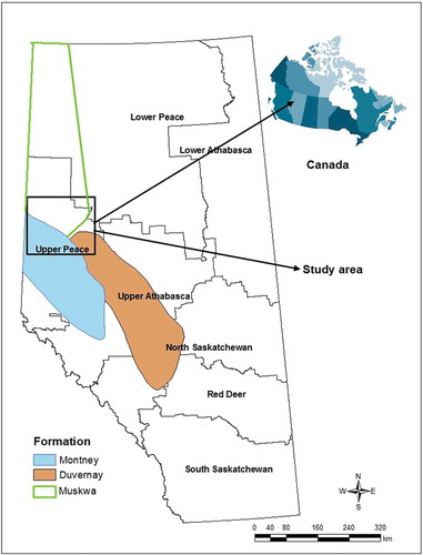
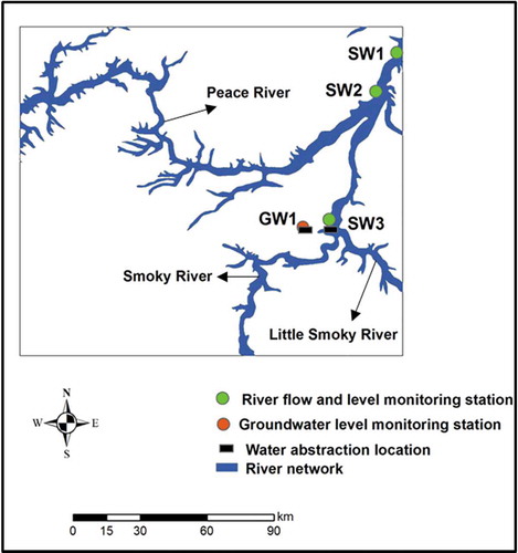
Figure 2. Surface water monitoring stations in the study area. Only one groundwater monitoring well is shown here as a water abstraction location for hydraulic fracturing.

The elevation of the study area is from 302 to 1024 m a.s.l., with an average slope of 2.1% (mean direction is southeast). Based on a 30-year period (1985–2014) of precipitation and temperature data, the mean annual precipitation and temperature in the study area are 423 mm (312 mm of rain and 111 mm of snow) and.1.9°C, respectively.

2.2 Modelling of GW–SW interaction

An integrated model was developed for the study area by using the MIKE-SHE and MIKE-11 models to investigate GW–SW interaction under the effects of water abstraction for hydraulic fracturing. MIKE-SHE is a physically based, distributed and structured grid-based hydrological model that simulates hydrological processes in a watershed under given hydrometeorological inputs. It simulates major components of the hydrological cycle, such as snow accumulation and snowmelt, evapotranspiration, unsaturated flow, saturated groundwater flow, overland flow and infiltration. The MIKE-SHE model domain was discretized into grid cells of 284 m × 284 m. Snowmelt was computed using the modified degree-day method. Overland flow was simulated using the finite difference method by solving the diffusive wave approximation of the St Venant equations. Unsaturated flow was computed using a two-layer water balance method due to the unavailability of detailed soil characteristics and geological layer data. Saturated groundwater flow was simulated using the finite difference method by solving the 3-D saturated groundwater flow equation. The saturated zone was divided into two layers in this study: an unconfined aquifer (situated over bedrock) and bedrock. MIKE-11 is a one-dimensional (1D) hydrodynamic model and it computes channel flow using the 1D St Venant equations. Channel flow was computed using an implicit finite difference scheme to solve the dynamic wave version of the St Venant equations. The MIKE-11 model was coupled with the MIKE-SHE model to simulate streamflow and stream water level along the channels and groundwater level in the aquifer under given hydrometeorological inputs. The exchange flow between the saturated zone and the stream was computed based on Darcy’s law. Details of the MIKE-SHE and MIKE-11 models are given in DHI (2009) and (DHI 2017), respectively.

The coupled MIKE-SHE and MIKE-11 model requires a number of inputs, such as watershed-specific data (elevation, channel geometry, soil type, and land use/land cover), hydrological data (streamflow, stream level and groundwater level), climate data (precipitation, temperature and reference evapotranspiration) and vegetation characteristic data (leaf area index and rooting depth). The details of these data for this study are provided in Table 1.

Table 1. Details of input data for the coupled MIKE-SHE and MIKE-11 model for the study area.

Data type	Data and format	Source
Watershed	Canadian Digital Elevation Data of 17.77 m grid	Natural Resources Canada
	Channel geometry	Digitizing digital elevation data and Google maps
	Land use/land cover of 30 m by 30 m grid for year 2000	Natural Resources Canada
	Soil	Alberta Environment and Parks
Hydrological	Daily streamflow from 2000 to 2012	Water Survey of Canada
	Groundwater level from 2000 to 2012	Alberta provincial groundwater monitoring wells database
Climate	Observed precipitation, temperature and reference evapotranspiration from 1986 to 2014	14 weather stations in the study area from Alberta Agroclimatic Information Service, and Alberta Environment and Sustainable Resource Development
Vegetation characteristics	Leaf area index and rooting depths of each land-use type	Task Committee on Hydrology Handbook (1996), Allen et al. (1998), Zeng (2001), Myneni et al. (2003), Kim et al. (2005), Wijesekara and Marceau (2009)

The initial potential head (groundwater table) maps in the aquifer (unconfined) and bedrock were prepared using observed groundwater table data collected from 1235 active and inactive monitoring wells in the study area from the Alberta provincial groundwater monitoring wells database and using the inverse distance weighted (IDW) interpolation method. In the IDW method, all of the data points are used to compute each interpolated value (Amidror 2002). The basic assumption of IDW is that the interpolated values should be affected more by nearby points and vice versa. Consequently, the interpolated value at each new point is a weighted average of the values of the scattered points, while the weight of the scatter point decreases as the distance from the interpolation point to the scatter point increases (Kurtzman and Kadmon 1999). Aquifer and bedrock lower level maps were prepared using bore log data of those wells in the study area and the IDW interpolation method. Around the perimeter of the study area, a no-flow boundary condition was assumed for the developed MIKE-SHE model for model simplicity and because of lack of information in the study area for setting appropriate boundary conditions (e.g. general head or specified head). For the MIKE-11 model, the no-flow boundary condition was chosen for all unconnected ends of the river branches except the Peace River, Smoky River and Little Smoky River because the upstream parts of these three large rivers (which are outside the study area) contribute, respectively, 88%, 8.1% and 2.3% of the flow at the outlet of the study area based on observed data at the monitoring stations of those areas. The boundary conditions at those upstream parts of three rivers were chosen as the inflow boundary. In addition, the downstream (Peace River) boundary of the model was chosen as the water level boundary based on the relationship between streamflow and water level. Before calibration, a sensitivity analysis of the modelling parameters was performed to determine which parameters are sensitive to the model outputs (streamflow, river water level, groundwater level). Horizontal hydraulic conductivity (loam) was found to be the most sensitive parameter. Horizontal hydraulic conductivity (clay loam), horizontal hydraulic conductivity (silty clay), specific storage (bedrock), specific yield (loam), evapotranspiration surface depth, water content at saturation (loam), degree-day melting coefficient, leakage coefficient of the bed material, channel roughness and overland surface roughness (forest) were placed as second to 11th sensitive parameters, respectively. Full details of the model set-up are provided in the Supplementary material.

The model was calibrated using automated calibration. The coupled model was calibrated and validated using observed climate data (precipitation, temperature and reference evapotranspiration) at monitoring weather stations, streamflow and river water levels at three monitoring stations, and groundwater levels at monitoring wells (only GW1 well is shown here) by changing the sensitive parameters. The coefficient of determination (R²) and coefficient of efficiency (NSE: Nash-Sutcliffe efficiency) were used to evaluate the goodness-of-fit of this hydrological model with the observed streamflow, river water and groundwater levels. The model calibration was performed from 1 January 2000 to 31 December 2006, and validation was performed from 1 January 2007 to 31 December 2012.

The coupled MIKE-SHE and MIKE-11 model estimated monthly total baseflow (groundwater discharge) in mm (area normalized flow) for the study area. The monthly baseflow was multiplied by the study area (km²) to get monthly volume of groundwater discharge. Finally, the monthly volume of groundwater discharge was divided by time to get mean monthly groundwater discharge. The mean monthly groundwater contribution to streamflow was calculated by dividing the mean monthly groundwater discharge by mean monthly streamflow simulated in the study area by the coupled MIKE-SHE and MIKE-11 model. In this study, environmental flow (Instream Flow Needs) during low-flow periods was also calculated using the Alberta Desktop method, which recommends that 80% exceedance of natural flow on the monthly time step is environmental flow (Alberta Environment and Alberta Sustainable Resource Development 2011). Environmental flow is the low-flow condition sustained by the groundwater discharge into the streams that provides ecosystem baseflow.

2.3 Hydraulic fracturing data collection and different water abstraction scenarios generation for hydraulic fracturing activities

Water-use data for hydraulic fracturing in 2013 and 2014 (Table 2) were collected from a publicly available source, Frac Focus Chemical Disclosure Registry (www.fracfocus.ca). Hydraulic fracturing data have been publicly available in Alberta since 19 December 2012 (Rivard et al. 2014). Hydraulic fracturing activities in 2013–2014 were conducted when oil and gas prices were relatively high (e.g. oil at USD$100/barrel in 2013–2014) (Ycharts Inc 2019). The annual water consumption in 2013 and 2014 was 997 291 and 948 931 m³, respectively.

Table 2. Monthly number of hydraulically fractured wells and water use in hydraulic fracturing in 2013 and 2014.

	Number of wells		Water used (m^3)
Month	2013	2014	2013	2014
January	18	20	43,714	66,865
February	29	19	97,466	43,309
March	10	35	15,535	78,858
April	3	9	5249	56,039
May	7	13	67,317	91,354
June	9	25	27,857	109,275
July	20	13	64,243	53,732
August	19	22	94,626	68,282
September	15	25	37,067	102,478
October	22	25	72,300	99,122
November	18	20	408,756	81,356
December	16	21	63,161	98,261

The publicly available data only report when and how much water was used in hydraulic fracturing. It does not include the time of water abstraction, how the water was transported to the site, the location of the source of water, what type of source, or whether any water was recycled. This constitutes a limitation in our study. To reduce these uncertainties the following assumptions were made:

• Consistent with Best and Lowry (2014), monthly water-use data in 2013–2014 were distributed in a temporally equal manner across all days of the particular month for numerical simulations.

• Only surface water (i.e. river), and a combination of surface water and groundwater was chosen as potential sources.

• When surface water was chosen as the sole source, it was assumed that all water was abstracted from one location near to the time of the fracking operations, and the location of water abstraction was chosen close to the monitoring river water level and flow station (SW3 station) so that the maximum impacts on river water level were estimated. The water abstraction location was assumed to be 1 km upstream of the SW3 station in the Smoky River (Fig. 2). This location was chosen because the SW3 station is situated in the Montney and Duvernay formations, and water abstraction from this location would have the maximum impacts on river water level fluctuations at the SW3 station.

• When both surface water and groundwater were chosen as the source, it was assumed all water was abstracted from one location in the river and one monitoring provincial groundwater well near the surface water abstraction location. The surface water abstraction location was assumed to be 1 km upstream of the SW3 station in the Smoky River. GW1 well is the only available active provincial groundwater monitoring well around the SW3 station. Best and Lowry (2014) used a municipal well close to the river network as water source for groundwater abstraction for hydraulic fracturing activities. Although monitoring wells are only pumped for sampling, groundwater monitoring well (GW1) was used here as a hypothetical scenario for pumping water for hydraulic fracturing activities because there is a lack of publicly available temporal groundwater levels data in the study area. The proportion of surface water and groundwater was determined from approved Alberta provincial water licenses for oil and gas activities in the region. Surface water is the most prevalent source (84%) of water used for oil and gas activities in the region (Alberta Environment 2007). Therefore, 84% water was attributed to abstraction from surface water, and the remaining water from groundwater.

• Recycling of flowback portion of either surface water or both surface water and groundwater used in hydraulic fracturing was considered as 15% which reflects best water management practices for the region. In the neighbouring province, British Columbia, Canada, 15% water used for hydraulic fracturing in 2013 was recycled water that came from flowback and produced water recycling (Goss et al. 2015).

Based on those assumptions, four potential scenarios of water abstraction in hydraulic fracturing were generated (Table 3). These scenarios do not provide exact prediction but provide the best estimate using the available data. The results represent the maximum probable effects on stream water and groundwater. These scenarios were used in the developed coupled model to compare the outputs with that of baseline scenario (i.e. no hydraulic fracturing). The effects of water abstraction (either from surface water (i.e. Smoky River) or both surface water and groundwater) for hydraulic fracturing in 2013 and 2014 were quantified using the coupled model by comparing the mean monthly and annual river water and groundwater levels, stream and groundwater flows, groundwater contributions to streamflow, and environmental flow during low-flow periods between the baseline scenario and various types of water abstraction scenarios for hydraulic fracturing activities.

Table 3. Different types of water abstraction scenarios for hydraulic fracturing activities.

Scenario	Water abstracted for hydraulic fracturing	Type of source water	Recycling of water
Baseline scenario	No hydraulic fracturing	-	No
Scenario 1	Water abstracted 1 km away from the SW3 station to the upstream direction from the Smoky River	Surface water (river) (100%)	No
Scenario 2	Water abstracted 1 km away from the SW3 station to the upstream direction from the Smoky River	Surface water (river) (85%)	Yes, 15%
Scenario 3	Water abstracted 1 km away from the SW3 station to the upstream direction from the Smoky River, and the GW1 well	Surface water (84%) and groundwater (16%)	No
Scenario 4	Water abstracted 1 km away from the SW3 station to the upstream direction from the Smoky River, and the GW1 well	Surface water (71.4%) and groundwater (13.6%)	Yes, 15%

3 Results and discussion

3.1 Results of model calibration and validation

Model calibration using monthly data (Fig. 3(a)) resulted in R² of 0.88 and NSE of 0.76 at the outlet (SW1 station) of the study area. Santhi et al. (2001) and Van Liew et al. (2003) suggested values of R² ≥ 0.6 and NSE ≥ 0.5 are acceptable for model evaluation. Moriasi et al. (2007) suggested that hydrological model simulation can be judged as satisfactory if NSE > 0.5 for monthly time step. Based on these evaluation statistics criteria, the developed model calibration was deemed satisfactory. The model validation (Fig. 3(b)) resulted in R² of 0.92 and NSE of 0.89 at the outlet of the study area using monthly data. As a result, satisfactory model validation was achieved. The model calibration and validation considering groundwater levels (at GW1 well here shown) also presented satisfactory results (Fig. 4). In addition, total water balance during the simulation period was also used as an indicator of the model performance. The total water balance error was less than 1% during both calibration and validation periods, which indicates an adequate model performance. The calculated R² and NSE values at other monitoring stations based on monthly streamflow, river water level, and groundwater level data are presented in Table 4.

Table 4. Performance statistics using observed and simulated streamflow, stream (i.e. river) water level and groundwater level data at various monitoring stations and wells during calibration and validation periods. R²: coefficient of determination; NSE: Nash-Sutcliffe efficiency criterion.

	Calibration			Validation
Monitoring station (measuring parameter)	R^2	NSE		R^2	NSE
SW1 (streamflow)	0.88		0.76	0.92	0.89
SW2 (river water level)	0.48		0.56	0.52	0.59
SW3 (streamflow)	0.92		0.63	0.9	0.75
SW3 (river water level)	0.91		0.71	0.86	0.65
GW1 (groundwater level)	0.71		0.69	0.75	0.81

Figure 3. Comparison of observed and simulated streamflow by the developed model at the SW1 station (outlet of the study area), and observed and simulated river water levels at the SW3 station during (a) calibration and (b) validation periods.

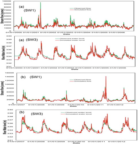
Figure 4. Comparison of observed and simulated groundwater levels by the developed model at the GW1 well during (a) calibration and (b) validation periods.

3.2 GW–SW interaction in response to water abstraction for hydraulic fracturing in 2013 and 2014

Similar to other previous studies, this study also found negative impacts of water abstraction for hydraulic fracturing on mean monthly and annual river water and groundwater levels, stream and groundwater flows, and environmental flow during low-flow periods. However, a positive impact was found on mean monthly and annual groundwater contributions to streamflow. The details of those results are presented and discussed in the following subsections.

3.2.1 Monthly and annual groundwater contributions to streamflow

The results showed that the increase in mean monthly groundwater contributions to streamflow occurred in all water abstraction scenarios for hydraulic fracturing activities in both 2013 and 2014 (Fig. 5) compared to the baseline scenario. The underlying causal mechanism is a change in gradient between the two systems (groundwater and surface water) due to the water abstraction during those scenarios. Saha et al. (2017a) found a change in gradient between surface water and groundwater played a role in changing groundwater contributions to streamflow under climate change scenarios. The major increase in mean monthly groundwater contributions to streamflow occurred when water was only abstracted from the surface water (Smoky River: Scenario 1). The increases are relatively small because of large study area. Surface water abstraction from 1 km away from the SW3 station in the Smoky River resulted in decreased surface water levels in the river reach of the Smoky River between the SW1 and SW3 stations and decreased adjacent groundwater levels (groundwater levels cannot be shown here because of 284 m grid cell). However, the minor decrease occurred in groundwater levels due to low groundwater velocity and low hydraulic conductivity of soils. Therefore, the gradient between the groundwater and surface water increased, and resulted in increased mean monthly groundwater contributions to streamflow.

Figure 5. Increase in mean monthly groundwater contributions to streamflow under various types of water abstraction scenarios for hydraulic fracturing in (a) 2013 and (b) 2014 compared to the baseline scenario.

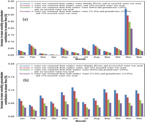
Table 5 presents the mean annual streamflow and groundwater discharge in the study area under the baseline scenario and various scenarios of water abstraction for hydraulic fracturing activities in 2013 and 2014. Under Scenario 1, the gradient was the highest due to more water abstraction from the surface water (Smoky River) compared to other scenarios, and therefore, greater increase in mean monthly groundwater contributions to streamflow occurred. These monthly increases were less than 0.35% (absolute value), which is not significant for this large study area. However, these increasing patterns of groundwater contribution to streamflow could be significant in a small catchment area where a large amount of water is extracted from the nearby river for hydraulic fracturing activities. With respect to the mean annual groundwater contribution to streamflow in 2013 and 2014 under the baseline scenario, the mean annual groundwater contribution to streamflow under all water abstraction scenarios for hydraulic fracturing increased very little (less than 0.1%) (Table 6).

Table 5. Mean annual streamflow, groundwater discharge and surface runoff generated in the study area under the baseline scenario and various scenarios of water abstraction for hydraulic fracturing in 2013 and 2014. Values in parentheses are absolute changes between various scenarios of water abstraction for hydraulic fracturing and the baseline scenario, in which “–” indicates a decrease with respect to the baseline scenario. Note, there is no change in surface runoff.

	2013			2014
Scenario	Mean annual streamflow (m^3/d)	Mean annual groundwater discharge (m^3/d)	Mean annual surface runoff (m^3/d)	Mean annual streamflow (m^3/d)	Mean annual groundwater discharge (m^3/d)	Mean annual surface runoff (m^3/d)
Baseline	2,310,941	1,179,014	1,131,927	2,032,906	1,152,835	880,071
Scenario 1	2,307,744 (–3197)	1,179,006 (–8)	1,131,927	2,029,882 (–3024)	1,152,825 (–10)	880,071
Scenario 2	2,308,224 (–2717)	1,179,009 (–5)	1,131,927	2,030,335 (–2570)	1,152,829 (–6)	880,071
Scenario 3	2,308,255 (–2685)	1,178,826 (–188)	1,131,927	2,030,365 (–2540)	1,152,435 (–400)	880,071
Scenario 4	2,308,658 (–2283)	1,178,838 (–176)	1,131,927	2,030,746 (–2159)	1,152,449 (–386)	880,071

Table 6. Mean annual groundwater contribution to streamflow under the baseline scenario and various scenarios of water abstraction for hydraulic fracturing in 2013 and 2014. Values in parentheses are absolute changes between various scenarios of water abstraction in hydraulic fracturing and the baseline scenario, in which positive values indicate an increase with respect to the baseline scenario.

Year	Baseline scenario	Scenario 1	Scenario 2	Scenario 3	Scenario 4
2013	51.02%	51.09% (0.07%)	51.08% (0.06%)	51.07% (0.05%)	51.06% (0.04%)
2014	56.71%	56.79% (0.08%)	56.78% (0.07%)	56.76% (0.05%)	56.75% (0.04%)

This increased groundwater contribution to streamflow under all water abstraction scenarios may result in some positive effects on stream water quality, such as cooler stream temperatures during warm months (i.e. months in late spring, summer and autumn), and warmer stream temperatures during cold months (i.e. winter and early spring) in the river reach between SW1 and SW3 stations (Price and Leigh 2006, Leigh 2010, The Freshwater Blog 2017). These results demonstrate that under Scenario 1 the above-mentioned effects would be higher as compared to other scenarios due to greater mean monthly and annual groundwater contributions to streamflow. Since the increase in mean monthly groundwater contribution to streamflow was less than 0.35%, the effects on stream temperature would not be significant. However, it could be significant in a small catchment area where large amount of water is extracted from the nearby river for hydraulic fracturing activities. These results also demonstrate that streamflow in the study area is more dependent on groundwater flow under Scenario 1 than under Scenario 4. Therefore, more annual water abstraction from the river for hydraulic fracturing activities could be possible under Scenario 4 than under Scenario 1 without causing a negative impact on regional groundwater level. It was also found that the mean annual groundwater contributions to streamflow under baseline and all water abstraction scenarios for hydraulic fracturing activities in 2013 were lower than those in 2014. This occurred because more precipitation occurred in 2013 (471 mm) than that in 2014 (312 mm). This increased precipitation resulted in increased surface water and groundwater levels in 2013. However, the greater increase occurred in surface water levels due to increased surface runoff because of the steep topography of the study area (elevation range from 302 to 1024 m). Therefore, the gradient between the groundwater and surface water decreased and resulted in lower mean annual groundwater contribution to streamflow in 2013. Similar results were found in Saha et al. (2017a, 2017b).

3.2.2 Monthly and annual river water levels and streamflow

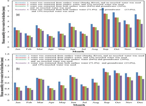
The maximum negative impact on mean monthly river water level occurred at the SW3 station (the width of the Smoky River at that site is approx. 230 m) in both 2013 and 2014 because water was abstracted 1 km away from the SW3 station to the upstream direction from the Smoky River. In 2013, the greatest (24.23 mm) and smallest (0.13 mm) mean monthly river water level declines occurred during November and April, respectively, due to the highest (408 756 m³) and lowest (5249 m³) water abstraction from the Smoky River (Scenario 1) during November and April, respectively (Fig. 6(a)). It was also found that Scenario 1 had the highest impact on river water level decline at the SW2 station (the width of the Peace River at that site is approx. 720 m) and SW3 station due to the highest water abstraction from the Smoky River (Fig. 6(a) and (b)). In contrast, Scenario 4 had the lowest impact on river water level decline at the SW2 and SW3 stations due to the lowest water abstraction from the Smoky River.

Figure 6. Mean monthly river water level declines compared to the baseline scenario at the (a) SW3 and (b) SW2 stations under various types of water abstraction scenarios for hydraulic fracturing in 2013.

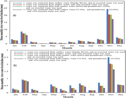
Figure 6 also illustrates that river water level declines varied significantly between the SW2 and SW3 stations. This occurred because the SW2 station is located approx. 54 km away from the SW3 station. Although mean monthly river water level declines were below 1 mm most of the year at the SW2 station, the mean monthly river water level declined 2.5 mm during November in Scenario 1 (Fig. 6(b)). This shows the potential impacts of water abstraction for hydraulic fracturing on river water level. At the annual scale, the mean annual river water level decline at the SW3 station in 2013 under scenarios 1, 2, 3 and 4 was 4.31, 3.63, 3.61 and 3.06 mm, respectively (Table 7). At the SW2 station, the declines were less than 0.64 mm. At the SW1 station (the width of the Peace River at that site is approx. 320 m and deeper than at SW2), which is located approx. 76 km away from the SW3 station, the impact was very low (<0.2 mm). However, in 2014 the highest (7.6 mm) and lowest (2.46 mm) river water level declines occurred during September and April, respectively (Fig. 7). The mean annual river water level decline at the SW3 station in 2014 under scenarios 1, 2, 3 and 4 was 4.57, 3.88, 3.86, and 3.29 mm, respectively (Table 7). At the SW2 and SW1 stations, these values were less than 0.76 and 0.3 mm, respectively.

Table 7. Mean annual river water level declines compared to the baseline scenario at the SW3 station under various types of water abstraction scenarios for hydraulic fracturing in 2013 and 2014.

Year	Mean annual river water level decline (mm)
	Scenario 1	Scenario 2	Scenario 3	Scenario 4
2013	4.31	3.63	3.61	3.06
2014	4.57	3.88	3.86	3.29

Figure 7. Mean monthly river water level declines compared to the baseline scenario at the (a) SW3 and (b) SW2 stations under various types of water abstraction scenarios for hydraulic fracturing in 2014.

The results also indicate that daily water abstraction for hydraulic fracturing activities was less than 1% of median streamflow at the SW1, SW2, and SW3 stations in 2013 and 2014. Barth-Naftilan et al. (2015) also found very low values because of higher watershed area and stream size. Similar to the results of Sharma et al. (2015), very little negative impact (<1%) on mean monthly and annual streamflow due to water abstraction for hydraulic fracturing was found at all stations in both 2013 and 2014.

3.2.3 Environmental flow during low-flow periods

It was found that water abstraction for hydraulic fracturing activities had negative impacts on environmental flow at the SW3 station during low-flow periods in 2013 (Jan.–Mar. and Nov.–Dec.). During low-flow periods, the water abstraction (surface water: Smoky River) was 63% of the total water abstraction in 2013. With respect to environmental flow in the Smoky River reach where the SW3 station is located during February and November under the baseline scenario, environmental flow during those months under all water abstraction scenarios for hydraulic fracturing decreased by 1.19–1.66%, and 3–4.17%, respectively (Table 8). The impacts at this river reach during January, March and December under all water abstraction scenarios were less than 1% compared to those under baseline scenario because of less water abstraction from the Smoky River and high value of environmental flow during those months under the baseline scenario. Although there was relatively high environmental flow in November under the baseline scenario, the highest (i.e. 408 756 m³) water abstraction from the river during this month resulted in highest decline in environmental flow. It was also found that Scenario 1 had the highest impact on environmental flow decline at the river reach where SW3 station is located due to the highest water abstraction from the Smoky River. Scenario 4 had the lowest impact on environmental flow decline at the river reach where SW3 station is located due to the lowest water abstraction from the Smoky River. This decreased environmental flow under all water abstraction scenarios may result in negative effects on aquatic ecosystems at the river reach where SW3 station is located during low-flow periods. When environmental flows at the Peace River reaches (where the SW1 and SW2 stations are located) during low-flow periods under the baseline scenario were compared with those under all water abstraction scenarios for hydraulic fracturing activities, environmental flow under all water abstraction scenarios for hydraulic fracturing decreased less than 0.1% compared to those under the baseline scenario because of very high value of environmental flow at the SW1 and SW2 stations (i.e. downstream reaches carry more flow than upstream reach, SW3) during those months under the baseline scenario. Therefore, the impacts on environmental flow not only depend on the amount of water abstraction for hydraulic fracturing activities from a particular cross-section of the river in a particular month, but also on the daily flow in that cross-section during that month. The results also indicated that water abstraction for hydraulic fracturing activities had negative impacts on environmental flow at the SW3 station during low-flow periods of 2014 (i.e. Jan.–Mar. and Sep.–Dec.). During low-flow periods, the water abstraction (surface water) was about 60% of the total water abstraction in 2014. With respect to environmental flow at the Smoky River reach where SW3 station is located during September and October under the baseline scenario, environmental flow during those months under all water abstraction scenarios for hydraulic fracturing decreased by 1.13–1.58%, and 0.9–1.17%, respectively (Table 8). The impacts at this river reach during January, February, March, November and December under all water abstraction scenarios were less than 1% compared to those under the baseline scenario because of high value of environmental flow during those months under the baseline scenario. Similar to 2013, Scenario 1 and Scenario 4 caused the highest and lowest impacts on environmental flow decline at the Smoky River reach where the SW3 station is located, respectively.

Table 8. Relative declines in environmental flow under various scenarios of water abstraction for hydraulic fracturing during low-flow periods in 2013 and 2014 with respect to the environmental flow under the baseline scenario.

Month	Scenario 1	Scenario 2	Scenario 3	Scenario 4
February 2013	1.66%	1.41%	1.4%	1.19%
November 2013	4.17%	3.54%	3.51%	3.0%
September 2014	1.58%	1.34%	1.32%	1.13%
October 2014	1.17%	1.05%	1%	0.9%

3.2.4 Monthly and annual groundwater levels and groundwater discharges

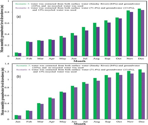
Figure 8 illustrates how mean monthly groundwater level drawdown changed compared to the baseline scenario at the GW1 well under various water abstraction scenarios for hydraulic fracturing in 2013 and 2014. Scenarios 1 and 2 are not shown because these scenarios only decreased adjacent groundwater levels and cannot be shown here because of 284 m grid size and a very small change in groundwater levels. In addition, they did not change groundwater level at the GW1 well because the GW1 well is located about 5.1 km away from the surface water abstraction location (i.e. 1 km away from the SW3 station to the upstream direction in the Smoky River). The drawdown increased in both scenarios 3 and 4 because of continuous groundwater pumping from the GW1 well. Scenario 3 had the highest drawdown (0.86 m) at the end of 2013 (Fig. 8(a)) because of more groundwater abstraction compared to Scenario 4. Best and Lowry (2014) reported similar drawdown at municipal well after one year of continuous pumping. In 2014, Scenario 3 also had the highest drawdown (1.26 m) at the end of 2014 (Fig. 8(b)). The results suggest groundwater abstraction for hydraulic fracturing could have significant effects on local groundwater level decline. Similar to streamflow, very little negative impact (less than 1%) on mean monthly and annual groundwater discharges (flows) due to water abstraction (surface water or both surface water and groundwater) for hydraulic fracturing was found in both 2013 and 2014.

Figure 8. Mean monthly groundwater level drawdown compared to the baseline scenario at the GW1 well under various types of water abstraction scenarios for hydraulic fracturing in (a) 2013 and (b) 2014.

3.3 Comparison of GW–SW interaction between 2013 and 2014

When mean monthly river water level declines at the SW3 station due to water abstraction for hydraulic fracturing, and the corresponding monthly water abstraction from the Smoky River in 2013 were compared with those in 2014 (only Scenario 1 shown), the higher the monthly water abstraction from the river in a particular month of 2013 and 2014, the higher the mean monthly river water level decline in that corresponding month was found in every month, except July and August (Table 9). This happened because lower soil moisture condition occurred due to lower precipitation in the study area during those 2 months in 2014 than that in 2013, which resulted in higher river water level declines in those 2 months of 2014. Although less water was abstracted in 2014, the mean annual river water level decline at the SW3 station in 2014 under scenarios 1, 2, 3 and 4 were more than those in 2013 by 026, 0.25, 0.25, and 0.23 mm, respectively, because of lower soil moisture conditions in 2014 resulting from lower precipitation in 2014 than that in 2013. Similar to 2013, the highest and lowest mean monthly river water level declines did not occur in 2014 during the highest and lowest water abstraction months from the river, respectively. These results demonstrate the significant effects of soil moisture for increasing river water level declines during lower soil moisture conditions, resulting in higher changes in gradient between the two systems (i.e. groundwater and surface water).

Table 9. Comparison of mean monthly river water level decline at the SW3 station and monthly water abstraction under Scenario 1 between 2013 and 2014.

Month	Mean monthly river water level decline under Scenario 1 (mm)		Difference in mean monthly river water level decline (mm) ^a	Monthly water abstraction from the Smoky River under Scenario 1 (m^3)		Difference in monthly water abstraction (m^3) ^b
	2013	2014		2013	2014
January	3.0	3.8	–0.8	43,714	66,865	–23,151
February	8.6	2.5	6.0	97,466	43,309	54,157
March	1.2	4.3	–3.0	15,535	78,858	–63,323
April	0.1	2.5	–2.3	5,249	56,039	–50,790
May	0.8	3.1	–2.3	67,317	91,354	–24,037
June	0.3	4.9	–4.5	27,857	109,275	–81,418
July	1.4	3.2	–1.8	64,243	53,732	10,511
August	2.3	4.4	–2.1	94,626	68,282	26,344
September	1.5	7.7	–6.2	37,067	102,478	–65,411
October	3.3	6.6	–3.4	72,300	99,122	–26,822
November	24.2	5.1	19.1	408,756	81,356	327,400
December	4.5	6.4	–1.9	63,161	98,261	–35,100

^amean monthly river water level decline in 2013 minus mean monthly river water level decline in 2014.

^bmonthly water abstraction from the Smoky River in 2013 minus monthly water abstraction from the Smoky River in 2014.

Groundwater level drawdown at the GW1 well at the end of 2014 was greater than that in 2013 (Fig. 8) even though there was less water pumped in 2014 than that in 2013. This occurred because precipitation was lower in 8 months of 2014 than that in 2013, and resulted in lower soil moisture in those months of 2014, which caused increased groundwater level drawdown in 2014. For example, in early July 2013 soil moisture content around the GW1 well was in between 0.4 and 0.44, whereas in 2014 that range was in between 0.36 and 0.4. Similar increased declines in groundwater levels due to groundwater pumping were reported by Cooper et al. (2015). The increased drawdown of groundwater level in lower soil moisture conditions also supported the importance of soil moisture condition for greater river water level declines. This shows the complexity nature of GW–SW interaction in the watershed. The change in mean annual groundwater contribution to streamflow, compared to the baseline scenario, under all water abstraction scenarios for hydraulic fracturing in 2014 was equal to or more than those in 2013 (Table 6) because of lower soil moisture conditions in 2014. Therefore, river water and groundwater levels decline as well as GW–SW interaction due to water abstraction for hydraulic fracturing would depend not only on the amount of water abstraction from the river or groundwater or both but also on future climate change induced variable precipitations, which would result in variable soil moisture conditions.

3.4 Potential and uncertainties regarding the results

The results of this modelling study present a comprehensive picture of regional GW–SW interaction under the impacts of water abstraction for hydraulic fracturing in a large study area. Based on having very small (<0.35%) negative impacts on temporal (i.e. monthly and annual) streamflow, groundwater discharges, river water and groundwater levels, a watershed manager can develop long-term seasonal and annual water abstraction plans for the river and groundwater for hydraulic fracturing in the study area. These very little negative impacts would provide useful information to other sectors (e.g. agricultural, forestry, fisheries, municipal) to expand their businesses in the study area because of having available water abundance in the study area. However, Cothren et al. (2013) found significant (67%) negative effects on streamflow due to water abstraction for hydraulic fracturing in one of the sub-basin of the Fayetteville Shale play in January 2008. Therefore, significant negative effects might occur in small catchment areas, and could create conflicts among water users especially in dry periods. Besides those negative impacts, a very small (<0.35%) positive impact of water abstraction for hydraulic fracturing on mean monthly and annual groundwater contributions to streamflow was found in our study, which would not result in significant impact on river water quality (i.e. stream temperature). However, significant positive impact could be possible in a small catchment area where large amount of water is abstracted from the nearby river for hydraulic fracturing activities. Therefore, further research should be done at a small scale (e.g. small catchment) to better understand and quantify the impacts of water abstraction from surface water (i.e. stream) and groundwater for hydraulic fracturing on groundwater contributions to streamflow in shale gas and oil play area. This small-scale research would identify how catchment area affect GW–SW interaction under the effects of water abstraction for hydraulic fracturing. In addition, various climatic regions should be considered for further case studies, especially in dry and arid climatic region, such as Texas, USA, where the impacts would be significant. In our study, the very little decrease of adjacent groundwater levels near to the surface water abstraction location in the Smoky River was not shown because of coarse grid size (284 m × 284 m). Therefore, finer grid resolution (e.g. 10 m × 10 m) of model domain should be used in a small catchment area to understand and visualize the impacts on groundwater level changes near to the surface water abstraction locations in streams for hydraulic fracturing activities.

Although the negative impacts on mean monthly and annual river water and groundwater levels, and stream and groundwater flows were very small (<0.35%), small (1–4.17%) negative impacts on environmental flow near the water abstraction location were found during low-flow periods (Table 8). This may result in negative effects on aquatic ecosystems in the river reach from where water was abstracted. However, very small (<0.1%) negative impacts were found in the downstream end of the water abstraction location. Since most water (i.e. approx. 63% and 60% water in 2013 and 2014, respectively) was abstracted during low-flow periods, water abstraction for hydraulic fracturing during low-flow periods should be done in the downstream of the study area, where very high value of environmental flows exist, in order to protect aquatic ecosystem from harmful impacts. The decreases in river water levels from near the water abstraction location to the downstream end of water abstraction location (Figs. 6 and 7) also support the necessity of water abstraction from the downstream of the study area during low-flow periods.

The water use in hydraulic fracturing is small compared to other water uses, such as irrigation, mining, manufacturing industries, municipal water supply (Kondash and Vengosh 2015). Therefore, the coupled modelling approach used in this study could be used to assess GW–SW interaction under the effects of water abstraction for those all water uses.

The results of this study have a number of limitations and uncertainties. First, due to lack of available data, a no-flow boundary condition was used for the MIKE-SHE model domain, which is the worst case scenario in comparison to use of general head or specified head boundaries. Based on the small impacts of water abstraction for hydraulic fracturing on groundwater and surface water, those impacts would be even smaller if a general or specified head boundary was used. Second, water abstraction scenarios for hydraulic fracturing were based on many assumptions. Although the assumptions were reasonable for the study area, more and better data would result in more accurate model results.

4 Conclusions

The modelling results demonstrate the effects of various water abstraction scenarios for hydraulic fracturing on temporal dynamics of GW–SW interaction by using a coupled MIKE-SHE and MIKE-11 model in a shale gas and oil play area of northwestern Alberta, Canada. The simulation results demonstrate that water abstraction for hydraulic fracturing has some negative impacts on mean monthly river water level and groundwater level declines depending on the amount of water abstraction from the river and groundwater well, respectively, and soil moisture conditions close to the water extracting sources. Although daily water abstraction for hydraulic fracturing activities was less than 1% of median streamflow at neighbouring monitoring sites, environmental flow during low-flow periods is negatively affected by water abstraction for hydraulic fracturing. The magnitude of the effects depends on the amount of water abstraction for hydraulic fracturing activities from a particular cross-section of the river in a particular month and the daily flow in that cross-section during that month. Although there were very small (<0.35%) negative impacts on mean monthly and annual river water and groundwater levels, and stream and groundwater flows, and small (1–4.17%) negative impacts on environmental flow near the water abstraction location during low-flow periods arising from water abstraction for hydraulic fracturing; there is a very small (<0.35%) positive impact of water abstraction for hydraulic fracturing on mean monthly and annual groundwater contributions to streamflow, which may result in positive effects on stream water quality. The results obtained from this study provide useful information for planning and regulating long-term seasonal and annual water abstractions from the river and groundwater for hydraulic fracturing activities in this large study area. Careful water management is required to maintain ecological conditions of the surface water and groundwater-dependent ecosystems.

Acknowledgements

The authors would like to thank the Associate Editor, Dr Corinna Abesser and an anonymous reviewer for providing their valuable comments and suggestions, which contributed a lot to improve this paper. The authors would like to thank Connie Van der Byl, Greg Chernoff, Linda Smith, Sonia Portillo, and Qiao Ying for their help. This study was funded by Institute for Environmental Sustainability, Mount Royal University.

Disclosure statement

No potential conflict of interest was reported by the authors.

Supplementary material

Supplemental data for this article can be accessed here.

Additional information

Funding

This work was supported by the Institute for Environmental Sustainability.

References

- Abbott, M.B., et al., 1986. An introduction to the European hydrological system – systeme hydrologique “SHE”, 1: history and philosophy of a physically based distributed modelling system. Journal of Hydrology, 87 (1–2), 45–59. doi:10.1016/0022-1694(86)90114-9
- Alberta Environment, 2007. Current and future water use in Alberta. Available from: http://www.assembly.ab.ca/lao/library/egovdocs/2007/alen/164708.pdf [Accessed 27 January 2016].
- Alberta Environment and Alberta Sustainable Resource Development, 2011. A desk-top method for establishing environmental flows in Alberta rivers and streams. Available from: http://aep.alberta.ca/water/programs-and-services/water-for-life/healthy-aquatic-ecosystems/documents/EstablishingEnvironmentalFlows-Apr2011.pdf [Accessed 15 October 2016].
- ALL Consulting, 2012. The modern practices of hydraulic fracturing: a focus on Canadian resources. Tulsa, Oklahoma: Prepared for Petroleum Technology Alliance Canada and Science and Community Environmental Knowledge Fund.
- Allen, R.G., et al., 1998. Crop evapotranspiration – guidelines for computing crop water requirements – FAO irrigation and drainage paper 56. Rome (Report): FAO – Food and Agriculture Organization of the United Nations.
- Amidror, I., 2002. Scattered data interpolation methods for electronic imaging systems: a survey. Journal of Electronic Imaging, 11 (2), 157–176. doi:10.1117/1.1455013
- Barth-Naftilan, E., Aloysius, N., and Saiers, J.E., 2015. Spatial and temporal trends in freshwater appropriation for natural gas development in Pennsylvania’s Marcellus Shale Play. Geophysical Research Letters, 42 (15), 6348–6356. doi:10.1002/2015GL065240
- BC Oil & Gas Commission, 2014. Application guideline for: deep well disposal of produced water, deep well disposal of nonhazardous waste. Available from: https://www.bcogc.ca/node/8206/download [Accessed 8 January 2020].
- Best, L.C. and Lowry, C.S., 2014. Quantifying the potential effects of high-volume water extractions on water resources during natural gas development: Marcellus Shale, NY. Journal of Hydrology: Regional Studies, 1, 1–16.
- Brittingham, M.C., et al., 2014. Ecological risks of shale oil and gas development to wildlife, aquatic resources and their habitats. Environmental Science & Technology, 48 (19), 11034–11047. doi:10.1021/es5020482
- Canadian Water Network, 2015. Water and hydraulic fracturing where knowledge can best support decisions in Canada. Available from: http://www.cwn-rce.ca/assets/resources/pdf/2015-Water-and-Hydraulic-Fracturing-Report/CWN-2015-Water-and-Hydraulic-Fracturing-Report.pdf [Accessed 10 July 2017].
- Cooper, D.J., et al., 2015. Effects of groundwater pumping on the sustainability of a mountain wetland complex, Yosemite National Park, California. Journal of Hydrology: Regional Studies, 3, 87–105.
- Cothren, J., et al., 2013. Integration of water resource models with Fayetteville Shale decision support and information system. University of Arkansas and Blackland Texas A&M Agrilife, Final Technical Report.
- DHI, 2009. MIKE SHE user manual. Vol. 2. Hørsholm, Denmark: Reference Guide.
- DHI, 2017. MIKE 11 a modelling system for rivers and channels. Hørsholm, Denmark: Reference Manual.
- Entrekin, S., et al., 2011. Rapid expansion of natural gas development poses a threat to surface waters. Frontiers in Ecology and the Environment, 9 (9), 503–511. doi:10.1890/110053
- The Freshwater Blog, 2017. How groundwater influences Europe’s surface waters. Available from: https://freshwaterblog.net/2017/01/13/how-groundwater-influences-europes-surface-waters/[Accessed 16th April 2018].
- Gallegos, T.J. and Varela, B.A., 2015. Trends in hydraulic fracturing distributions and treatment fluids, additives, proppants, and water volumes applied to wells drilled in the United States from 1947 through 2010 – data analysis and comparison to the literature. U.S. Geological Survey Scientific Investigations. Report 2014–5131, 15. doi:10.3133/sir20145131.
- Goss, G., et al., 2015. Unconventional wastewater management: a comparative review and analysis of hydraulic fracturing wastewater management practices across four North American basins. Available from: http://www.cwn-rce.ca/assets/resources/pdf/Hydraulic-Fracturing-Research-Reports/Goss-et-al.-2015-CWN-Report-Unconventional-Wastewater-Management.pdf. [Accessed 15 December 2016].
- Kargbo, D.M., Wilhelm, R.G., and Campbell, D.J., 2010. Natural gas plays in the Marcellus shale: challenges and potential opportunities. Environmental Science & Technology, 44 (15), 5679–5684. doi:10.1021/es903811p
- Kennedy, M., 2011. BC oil & gas commission – experiences in hydraulic fracturing. Warsaw, Poland: Ministry of Economy.
- Kim, S.H., et al., 2005. Analysis of temporal variability of MODIS leaf area index (LAI) product over temperate forest in Korea. International Geoscience and Remote Sensing Symposium (IGARSS), 6, 4343–4346.
- Kondash, A. and Vengosh, A., 2015. Water footprint of hydraulic fracturing. Environmental Science & Technology, 2, 276–280.
- Kurtzman, D. and Kadmon, R., 1999. Mapping of temperature variables in Israel: a comparison of different interpolation methods. Climate Research, 13, 33–43. doi:10.3354/cr013033
- Leigh, D.S., 2010. Hydraulic geometry and channel evolution of small streams in the Blue Ridge of western North Carolina. Southeastern Geographer, 50 (4), 394–421.
- Moriasi, D.N., et al., 2007. Model evaluation guidelines for systematic quantification of accuracy in watershed simulations. American Society of Agricultural and Biological Engineers, 50 (3), 885–900.
- Myneni, R., et al., 2003. User’s guide FPAR, LAI (ESDT: MOD15A2) 8-day composite NASA MODIS land algorithm, FPAR. LAI User’s Guide, Terra MODIS Land Team (Report).
- Naumburg, E., et al., 2005. Phreatophytic vegetation and groundwater fluctuations: a review of current research and application of ecosystem response modeling with an emphasis on great basin vegetation. Environmental Management, 35 (6), 726–740. doi:10.1007/s00267-004-0194-7
- Price, K. and Leigh, D.S., 2006. Morphological and sedimentological responses of streams to human impact in the southern Blue Ridge mountains, USA. Geomorphology, 78 (1–2), 142–160. doi:10.1016/j.geomorph.2006.01.022
- Rahm, B.G. and Riha, S.J., 2012. Toward strategic management of shale gas development: regional, collective impacts on water resources. Environmental Science & Policy, 17, 12–23. doi:10.1016/j.envsci.2011.12.004
- Rivard, C., et al., 2014. An overview of Canadian Shale gas production and environmental concerns. International Journal of Coal Geology, 126, 64–76. doi:10.1016/j.coal.2013.12.004
- Rokosh, C.D., et al., 2012. Summary of Alberta’s shale and siltstone hosted hydrocarbon resources potential (ERCB/AGS Open File Report No. 2012--‐06). Edmonton: ERCB (Energy Resources Conservation Board) and AGS (Alberta Geological Survey).
- Saha, G.C., et al., 2017a. Temporal dynamics of groundwater-surface water interaction under the effects of climate change: a case study in the Kiskatinaw River Watershed, Canada. Journal of Hydrology, 551, 440–452. doi:10.1016/j.jhydrol.2017.06.008
- Saha, G.C., Li, J., and Thring, R.W., 2017b. Understanding the effects of parameter uncertainty on temporal dynamics of groundwater-surface water interaction. Hydrology, 4 (2), 28. doi:10.3390/hydrology4020028
- Santhi, C., et al., 2001. Validation of the SWAT model on a large river basin with point and nonpoint sources. Journal of the American Water Resources Association, 37 (5), 1169–1188. doi:10.1111/j.1752-1688.2001.tb03630.x
- Shank, M.K. and Stauffer, J.R., 2015. Land use and surface water withdrawal effects on fish and macroinvertebrate assemblages in the Susquehanna River basin, USA. Journal of Freshwater Ecology, 30 (2), 229–248. doi:10.1080/02705060.2014.959082
- Sharma, S., et al., 2015. Hydrologic modelling to evaluate the impact of hydraulic fracturing on stream low flows using SWAT model: a case study of muskingum watershed in Eastern Ohio. American Journal of Environmental Sciences, 11 (4), 199–215. doi:10.3844/ajessp.2015.199.215
- Shrestha, A., et al., 2016. Scenario analysis for assessing the impact of hydraulic fracturing on stream low flows using the SWAT model. Hydrological Sciences Journal, 62 (5), 849–861. doi:10.1080/02626667.2016.1235276
- Sophocleous, M., 2002. Interactions between groundwater and surface water: the state of the science. Hydrogeology Journal, 10 (1), 52–67. doi:10.1007/s10040-001-0170-8
- Su, X., et al., 2017. Biogeochemical zonation of sulfur during the discharge of groundwater to lake in desert plateau (Dakebo Lake, NW China). Environmental Geochemistry and Health, 5, 1–16.
- Task Committee on Hydrology Handbook, 1996. Hydrology handbook prepared by the task committee on hydrology handbook of management group D of the American Society of Civil Engineers. 2nd ed. New York: ASCE.
- Van Liew, M.W., Arnold, G., and Garbrecht, J.D., 2003. Hydrologic simulation on agricultural watersheds: choosing between two models. Transactions of the American Society of Agricultural Engineers, 46 (6), 1539–1551. doi:10.13031/2013.15643
- Vengosh, A., et al., 2014. A critical review of the risks to water resources from unconventional shale gas development and hydraulic fracturing in the United States. Environmental Science & Technology, 48 (15), 8334–8348. doi:10.1021/es405118y
- Wang, W., et al., 2016. A quantitative analysis of hydraulic interaction processes in stream-aquifer systems. Scientific Reports, 6 (1), 19876. doi:10.1038/srep19876
- Wijesekara, G.N. and Marceau, D.J., 2009. Integrating a land-use cellular automata (CA) model with a hydrological model (MIKE-SHE) to simulate the impact of land use changes on water resources in the elbow river watershed in Southern Alberta. Report Submitted to Alberta Environment.
- Ycharts Inc, 2019. Average crude oil spot price. Available from: https://ycharts.com/indicators/average_crude_oil_spot_price [Accessed 22 March 2019].
- Zeng, X., 2001. Global vegetation root distribution for land modeling. Journal of Hydrometeorology, 2 (5), 525–530. doi:10.1175/1525-7541(2001)002<0525:GVRDFL>2.0.CO;2