Projection of runoff characteristics as a response to regional climate change in a Central/Eastern European catchment

ABSTRACT

The impact of climate change on runoff characteristics is investigated for the Upper Tisza basin, in eastern Central Europe. For a reliable estimation of uncertainty, an appropriate stochastic weather generator is embedded into a Monte Carlo cycle capable of generating any large number of independent, equally probable, 100-year-long daily sequences of synthetic data with which a hydrological model is driven in order to obtain the hydrological responses to the meteorological data sequences. According to our results, a decrease of daily average runoff is likely to occur in the future in the Upper Tisza basin, especially in July and August. The occurrence of water levels below the critical low level is estimated to increase between July and October. Level-3 flood warnings are projected to be less frequent in the future; however, they will tend to be more severe than in the historical period.

KEYWORDS:

• runoff
• DIWA model
• climate simulation
• level-3 flood warning
• critical low water level
• Upper Tisza catchment

Editor A. Fiori;Associate editor not assigned

Introduction

Both climate change studies and analyses of the effects of climate change on different sectors, i.e. hydrology, agriculture, ecology, tourism, have been highlighted in recent years (e.g. Rosenzweig and Parry 1994, Prudhomme et al. 2010, Wheeler and von Braun 2013, Dirks et al. 2015, Hansen and Cramer 2015, Gosling and Arnell 2016, Wu et al. 2016, Eisner et al. 2017, Joseph et al. 2018, Evans 2019). These issues are quite pertinent because global climate change implies that not only higher temperature values but also extreme weather events will tend to occur more frequently (IPCC 2012), which may result in different natural, economic and environmental damage. In order to mitigate the potential hazards, adaptation strategies (e.g. Filho et al. 2018, Wiréhn 2018) need to be developed in time. Reliable impact studies will serve as evidently necessary key inputs for the development of appropriate national and local adaptation strategies (Challinor et al. 2018).

The projected precipitation and temperature changes may have a substantial effect on water-related issues, i.e. the quality and quantity of drinking water (Depla et al. 2009), sustainable agriculture (Wiebe et al. 2015), shipping (Becker et al. 2018) and hydropower (van Vilet et al. 2016). Possible hydrological responses to climate change are analysed and discussed on the basis of hydrological models for which climate projections provide inputs (e.g. Cameron et al. 2000, Dankers and Feyen 2008, Teutschbein and Seibert 2010, 2012, Hanel et al. 2012, Rojas et al. 2012, Hirabayashi et al. 2013, Teutschbein 2013, Piras et al. 2014, Li et al. 2015, Karlsson et al. 2016, Kour et al. 2016, Nerantzaki et al. 2019).

There is growing scientific and public concern about flood events in Europe, as they have become more frequent and more severe in a number of locations (Kundzewicz et al. 2013a, 2019, Hall et al. 2014); moreover, the losses due to flood disasters have also increased (Kundewicz et al. 2013b). Altogether, 3563 floods were recorded in 37 European countries between 1980 and 2010 (the record year was 2010, with 321 floods), with annual flood losses being projected to increase. These changes have been dominantly induced by socio-economic development and climate change. In the European Union (EU), a framework was set up to reduce the risks of floods: Directive 2007/60/EC¹ on the assessment and management of flood risks. This states clearly the importance of taking into account climate change in the case of long-term developments. Due to climate change and urbanization, more uncertainty has emerged; hence, continuous monitoring has been proposed in order to help minimize the potential damage (EC 2019). The European Council is promoting natural water retention measures to mitigate flood hazards. Almost every member state (27 out of 28) treats floods as a major natural hazard, which seems necessary, as Rojas et al. (2013) projected a significant increase in the cost of flood-related damages by 2080. The EU Water Framework Directive (2000/60/EC) also helps to manage the effects of climate change by anticipating more floods and more droughts.

A shift can already be seen in the timing of floods in Europe in the 1960‒2010 time period (Blöschl et al. 2017). Considering the future, according to Dankers and Feyen (2008), extreme river discharges are likely to occur in Europe in summer and autumn. Nevertheless, floods will be less frequent in Northern, Central and Eastern Europe because of the projected decline of snowfall, which is verified by the analysis of Rojas et al. (2012) among others. However, Kundewicz et al. (2016) found that there are discrepancies between the results of different studies focusing mainly on the northern parts of the continent, as snowmelt and rainfall floods are also likely to occur – both being estimated to increase according to climate projections. Flood levels are projected to increase south of 60°N in Europe, which implies significant changes in the majority of cases. Within Europe, the flood and drought-related impacts of +2°C global warming are estimated to be the most severe in France and Spain (Roudier et al. 2016). Several studies have investigated the relationship between floods and the climate change projections of extreme precipitation events, which are summarized in Madsen et al. (2014). In general, an increase in extreme precipitation is predicted, while in the case of extreme discharge, the projected changes do not reach such a clear conclusion, with both positive and negative trends being possible. Nevertheless, it can be concluded overall that the number of snowmelt-induced floods is likely to decrease in the future due to higher temperatures. Huang et al. (2013) assume a declining future trend in the flood levels of most rivers in Germany, although the uncertainty of these estimations was quite high. It can be concluded that snow melting plays a key role in Polish and Norwegian catchments (Meresa et al. 2017), as well as in Switzerland, where decreasing summer precipitation additionally affects flood seasonality (Köplin et al. 2014).

Considering the methodology, most of the studies apply an adequate hydrological model to simulate precipitation runoff processes; some examples of recent hydrological studies are briefly summarized in Table 1. Climate simulations are used to provide the necessary meteorological input data for the future time period: regional climate models (RCMs) embedded in global climate models (GCMs) or solely GCMs without dynamical downscaling. Recent studies usually apply CORDEX (Coordinated Regional Climate Downscaling Experiment) simulations that take into account representative concentration pathway (RCP) emissions scenarios (e.g. Bisselink et al. 2018, Lobanova et al. 2018), while studies drawn up less recently used the SRES scenarios (Special Report on Emissions Scenarios of the Intergovernmental Panel on Climate Change, IPCC) (e.g. Radvánszky and Jacob 2008, Huang et al. 2013, Gosling and Arnell 2016). It is possible to use raw climate simulations for impact studies; however, as climate projections usually contain biases, it is advisable to apply a bias-correction technique to the raw simulation data prior to input into the hydrological model. The bias correction of RCM simulations is still a critical issue (Ehret et al. 2012, Maraun 2016), but it is usually recommended for impact studies, as the reliability of climate model outputs is especially important in these cases (Rojas et al. 2011, Andrej and Kajfez-Bogataj 2012, Muerth et al. 2013, Olsson et al. 2013, Addor and Seibert 2014). The most common methods are (a) the delta method, which is based on a simple shift/scaling (e.g. Lehner et al. 2006, Hanel et al. 2012, Hall et al. 2014, Gosling and Arnell 2016, Marhaento et al. 2018, Wang et al. 2019); (b) quantile mapping, which is based on fitting the distribution functions (e.g. Hagemann and Dümenil 1998, Chen et al. 2011, Rojas et al. 2011, Ahmed and Tsanis 2016, Lobanova et al. 2018, Marhaento et al. 2018); and (c) the use of a stochastic weather generator (SWG) (Chen et al. 2011, Kay and Jones 2012, Teutschbein 2013, Hall et al. 2014) or a rainfall model (Cameron et al. 2000), both being able to generate several possible climate scenarios.

Table 1. Some examples of recent hydrological studies for different target areas. The hydrological and climate models applied to the analysis, the emissions scenario, the main results and the references are also indicated.

Hydrological model	Climate model (scenario)	Target area	Main results	Reference
AMUNDSEN	31 EURO-CORDEX simulations (RCP2.6, RCP4.5, RCP8.5)	Venter Ache, Rofenache, Vernagtbach, Gurgler Ache, Gepatschalm, Taschachbach, Pitze catchments (Ötztal Alps, Austria)	Decrease of runoff	Hanzer et al. (2018)
BILAN	15 ENSEMBLES simulations (A1B)	250 catchments in the Czech Republic	Increase in winter runoff, decrease in summer and spring	Hanel et al. (2012)
HBV	11 ENSEMBLES simulations (A1B)	Storbacken, Tannfors, Vattholmaan, Brusaan, Ronne catchments (Sweden)	Reduction of spring floods, increase in autumn flood peaks	Teutschbein and Seibert (2012)
HSAMI	CGCM, CRCM (A2, B1)	Manicouagan catchment (Canada)	Increase in winter (Nov-April), decrease in summer discharge	Chen et al. (2011)
HBV	8 NARCCAP simulations (A2)	Spencer Creek catchment (Canada)	Increase in daily average flow in winter, decrease in the other seasons. Increase in high flows, decrease in low flows	Ahmed and Tsanis (2016)
	7 EURO-CORDEX simulations (RCP4.5, RCP8.5)	Nysa Klodzka, Wisla, Dunajec, Biala Tarnowska, Olesnica, Mysla, Flinta, Guber, Narewka (Poland)	Increase in flood indices	Osuch et al. (2017)
Karst-SWAT	11 EURO-CORDEX simulations (RCP2.6, RCP4.5, RCP8.5)	Crete	Decrease in surface and karstic flows in spring	Nerantzaki et al. (2019)
LISFLOOD	12 ENSEMBLES simulations (A1B)	Europa	Reduction in snowmelt-induced floods	Rojas et al. (2012)
	HIRHAM (A2)	Europa	General increase of the magnitude and frequency of extreme discharge levels, decrease in the northeast	Dankers and Feyen (2008)
Mac-PDM.09	21 CMIP3 GCM simulations (B1, B2, A1B, A2)	1339 watersheds (Global)	Increase in exposure of water scarcity	Gosling and Arnell (2016)
MPI-HM; LPJmL	ECHAM5, CNRM-CM3, IPSL CM4 (A2, B1)	Global	Differences between the signals of runoff changes considering raw and bias-corrected GCM data	Hagemann et al. (2011)
PDM	29 UKCP09 simulations (A1B)	Helmsdale, Findhorn, Eden, Leet Water, Bure, Mimram, Avon, Yealm, Teme (UK)	Increase in 20-year return period flood peaks	Kay and Jones (2012)
SWAT	RegCM4 and 6 GCM simulations (RCP4.5, RCP8.5)	Samin catchment (Indonesia)	Reduction of surface runoff, increase of baseflow	Marhaento et al. (2018)
SWIM	REMO [1], CCLM[2], Wettreg [3] (A2, B1, A1B)	Danube, Elbe, Ems, Rhine, Weser catchments (Germany)	Extension of flood season by [1, 2], declining trend in flood level by [3]	Huang et al. (2013)
	7 EURO-CORDEX simulations (RCP4.5, RCP8.5)	Tagus, Eman and Lule, Rhine, Danube, Teteriv, Tay, Northern Dvina (Europe)	South: decrease in water availability, North: increase	Lobanova et al. (2018)
	7 CORDEX simulations (RCP4.5, RCP8.5)	Teteriv, Upper Western Bug, Samara catchments (Ukraine)	Earlier spring flow	Didovets et al. (2017)
Topkapi	REMO, RegCM3, ECHAM5 (A1B)	Upper-Rhone catchment (Switzerland)	Increase of daily max. flows, decrease discharge in August-Sept.	Fatichi et al. (2015)
TOPMODEL	HadCM2 (UKCIP98)	Wye catchment (UK)	Small changes	Cameron et al. (2000)
WASMOD-D	RegCM4 (RCP4.5)	South-Africa	Decrease in runoff, except for the eastern part	Li et al. (2015)
WaSiM	ALADIN, WRF (A1B, RCP8.5)	Brixental catchment (Austria)	Decrease of the mean annual streamflow	Strasser et al. (2019)
WaterGAP	HadCM3, ECHAM4 (Baseline-A water use scenario)	Europa	North: 100-year floods more frequent; south: increase of drought	Lehner et al. (2006)
WetSpa	KNMI, MPI (A1B)	Váh, Laborec catchments (Slovakia)	Increase in extremes during flood events	Kohnová et al. (2019)

In this study, an SWG embedded in a Monte Carlo (MC) cycle was used, which can be an appropriate tool to measure uncertainty. Kay and Jones (2012) compared simulation results regarding flood frequency based on different meteorological inputs. They found that using a weather generator (WG) has greater impact than an RCM ensemble. Smith et al. (2014), as well as Cameron et al. (2000), used the GLUE (Generalized Likelihood Uncertainty Estimation) approach, and they reject the single optimum concept and approve that several parameter sets can exist, so they also applied an MC procedure. Using an MC simulation to generate several time series is quite common in hydrological studies (e.g. Cameron et al. 2000, Diaz-Ramirez et al. 2012, Charalambous et al. 2013, Sordo-Ward et al. 2016, Chen et al. 2017, Wang et al. 2017, Wang and Wang 2019, Annis et al. 2020).

Among European countries, Hungary is especially exposed to inland floods due to its relatively low elevation above sea level and the large rivers (the Danube and Tisza are the two major rivers) flowing through the country, together with their tributary systems from the hills and mid-level mountains. Within the whole Central European area, the highest relative proportion of people living in flood-prone areas (18% of the population) can be found here (EEA 2016). These facts are forcing our analysis, which focuses on the effects of climate change on runoff characteristics in a relatively small catchment in the region, namely the Upper Tisza catchment (shared by Hungary, Ukraine and Romania) with the use of an SWG to estimate the potential future climate simulated by an RCM and a hydrological model to simulate runoff processes. The SWG is used to represent the uncertainty of climatic conditions. Bias-corrected meteorological elements are provided by an RCM simulation to generate several potential simulations with equal probability. Therefore, the uncertainty of estimations for the recent past and for the future can also be assessed, which is a key aspect of our modelling concept, and which, despite its importance, is not yet sufficiently common in hydrological design practices.

The uncertainty (which arises from multiple sources) is quite high in impact studies, so it is high the case of hydrological studies as well, while it is usually based on a complex model chain. First of all, selection of the hydrological model brings uncertainty to the investigation (e.g. which processes are included or omitted). Secondly, the meteorological time series are key input data; therefore, the choice of climate simulation is also critical (Hawkins and Sutton 2011). For smaller regions, RCMs are advisable, in which case, the driving GCM also introduces uncertainty. Furthermore, the RCM itself, the future emissions scenario it takes into account and the potentially applied bias-correction method mean uncertainty as well (Garner et al. 2015, Clark et al. 2016). Muerth et al. (2012) investigated which factor plays the more important role in uncertainty, to which end they selected one component to vary in the actual analysis, while the others remained fixed. According to their results, simulated values for the future highly depend on the applied GCM or GCM-RCM set-up and the hydrological model, while in the case of historical simulations, the applied bias-correction method is the key factor. Giuntoli et al. (2015) concluded that the greatest source of uncertainty is GCMs, except for snow-dominated regions, where the hydrological models are critical. Hutchins et al. (2016) suggest that only the relative changes are presented in the case of simulations rather than absolute values in order to avoid bias-related misleading conclusions. Clark et al. (2016) emphasized that uncertainty related to poor models and methods and internal climate variability is usually neglected and they suggested to move beyond the common climate change scenario ensembles, which are based on a collection of models and methods with known problems. In our study, climate variability is taken into account as the meteorological time series provided by the WG embedded in an MC cycle gives all the possible climate realizations.

In the following sections, the data and the hydrological model are briefly presented. The applied methodology and the target domain are described in sections 4 and 5, respectively. Our results are shown and discussed subsequently. Finally, the main conclusions are drawn.

Data

In this study, meteorological data (distributed daily precipitation sum, minimum and mean temperature) were necessary to serve as boundary condition data for the distributed hydrological model in a Lambert azimuthal equal-area (LAEA) projection system at 1 km × 1 km resolution. The reference meteorological database was the CARPATCLIM (Szalai et al. 2013), as it is the only freely available database with high spatial resolution based on observations from several hundred stations within the Carpathian Basin. These station data are homogenized by applying the MASH software (Szentimrey 2007) and, then, the homogenized station data are interpolated to a horizontal grid with 0.1° resolution (44°‒50°N; 17°‒27°E) using the MISH method (Szentimrey and Bihari 2006). Considering time, the CARPATCLIM database covers the time period 1961–2010 on a daily basis. Basically, the database contains 16 meteorological variables and several climate indices as well.

In order to make estimations for the future, climate projections are needed. As the target domain is relatively small, we used an RCM simulation in this study, with 0.11° horizontal resolution. We chose the RegCM4 model (Elguindi et al. 2011) because, it was adapted and run at the Department of Meteorology, Eötvös Loránd University (Pieczka et al. 2017) in the framework of the Med-CORDEX programme.² The RegCM4 model is a hydrostatic, sigma coordinate, primitive equation model. It has open-source, user-friendly code and was the first limited-area model, which was developed for long-term simulations. The model dynamics encompasses the horizontal momentum, the continuity, the thermodynamic and the hydrostatic equations. Furthermore, RegCM4 applies different parameterizations, e.g. radiation scheme (Kiehl et al. 1996), planetary boundary layer scheme (Holtslag et al. 1990), land surface models (Dickinson et al. 1993), ocean flux parameterization (Zeng et al. 1998), prognostic sea-surface skin (Zeng 2005), lake model (Hostetler et al. 1993) and chemistry model (Alfaro and Gomes 2001, Laurent et al. 2008). For large-scale precipitation, RegCM4 uses SUBEX (Sundqvist et al. 1989), while in the case of convective precipitation, a mixed scheme is applied: Emanuel (1991) over sea and Grell (1993) over land with Fritsch and Chappell (1980) closure. The RegCM4 simulation used in this study covers the area delimited by 43.8°‒50.6°N and 6°‒29°E, including the Upper Tisza catchment. It embraces 130 years, from 1970 to 2099 with a daily time step. The historical run is defined until 2005 with observed greenhouse gas (GHG) concentrations. For the future (from 2006 to the end of the 21st century) the RCP8.5 scenario (van Vuuren et al. 2011) is taken into account as it has the highest anthropogenic effect among the available scenarios. According to this quite pessimistic scenario, the radiation forcing will increase by 8.5 W/m² by 2100 compared to the pre-industrial era, implying that the atmospheric concentration of GHGs will continuously increase in the 21st century until it reaches about 1250 ppm CO₂-equivalent in 2100. Furthermore, the population and the usage of renewable energy are also assumed to grow. The ratio of croplands and pastures is estimated to increase, while natural vegetation cover is projected to decline. To run the RegCM4 model with 0.11° resolution, the necessary initial and boundary conditions were provided by the 50-km experiment of RegCM4 (Pieczka et al. 2019), which was driven by the global HadGEM model (Collins et al. 2011).

In order to use the RegCM4 model simulation data for the hydrological simulations, it was necessary to first transform the coordinates of the RegCM4 model into the LAEA (Lambert Azimuthal Equal-Area) system. Finally, the RegCM4 model data were downscaled to 1 km × 1 km resolution, using variogram analysis and kriging (Cressie 1985, Amani and Lebel 1997).

A brief overview of the hydrological model

In this study, the spatially distributed, physically based DIstributed WAtershed (DIWA) hydrological model (Szabó 2007) and its software system, DIWA-HFMS (Hydrologic Forecasting & Modelling System), were used. The DIWA model (Fig. 1) takes into account all the fundamental hydrological processes, namely, precipitation, interception, evaporation, transpiration, infiltration, soil water redistribution, snow accumulation, snow melting, and surface, subsurface and channel runoff. In this study the DIWA model divides the catchment into 1 km × 1 km cells (in the LAEA projection system), which are assumed to be homogeneous and neighbouring cells are related to each other according to the runoff hierarchy. Cells can be basically characterized by three layers: the atmosphere, the vegetation and the soil.

Figure 1. Flowchart of the DIWA hydrological model.

Hydrological processes are clearly determined by the characteristics of the catchment, such as climate, topography, soil and vegetation type, or of the land use, among which there are some properties that can be assumed as constants, while others are quite variable within the year. Therefore, the DIWA model distinguishes between permanent and seasonally changing factors. For example, an important permanent factor is topography. The potential capacity of interception and evapotranspiration shows seasonality, as the annual cycle of vegetation has an important role in these processes. So, the DIWA model takes into account intra-annual characteristics, e.g. the monthly leaf area index (LAI), which is determined by the land use and the monthly normalized difference vegetation index (NDVI) provided by satellite data (Tucker 1979).

Consequently, the DIWA model needs different input data to complete hydrological simulations. In this study, meteorological data inputs are provided basically by CARPATCLIM and RegCM4. Data regarding the topography are provided by the digital elevation model (DEM), which was downloaded from the homepage of the US Geological Survey, Earth Resources Observation & Science (USGS EROS). For the land-use coverage, the CORINE database³ is applied, which distinguishes 45 different land-use types. The monthly average LAI (Pistocchi 2015) is downloaded from the EU JRC Data Catalogue.⁴ The soil data (Panagos et al. 2012) are from the European Soil Data Centre (ESDAC).⁵

According to the principal concept of the DIWA model, if daily mean temperature is below 0°C, precipitation is considered to form as snow. Snow melting is calculated by the degree-day factor method (Martinec 1960, Martinec and Rango 1986):

(1) $M=a\cdot (T_{\mathrm{m}\mathrm{e}\mathrm{a}\mathrm{n}}-T_{\mathrm{c}\mathrm{r}\mathrm{i}\mathrm{t},M})$(1)

where M (mm) is the daily rate of snowmelt depth, a (mm °C⁻¹ d⁻¹) is the degree-day factor, T_mean (°C) is the daily mean temperature and T_crit,M (°C) is the critical temperature of melting.

It is important to estimate the sum of precipitation that directly reaches the surface; therefore, land-use-dependent interception also has to be taken into account. The DIWA model calculates the retained water amount on the vegetation surface at the end of a time interval, Δt, as:

(2) $S_{I,\mathrm{\Delta }t}=S_{I,\mathrm{m}\mathrm{a}\mathrm{x}}-\left(S_{I,\mathrm{m}\mathrm{a}\mathrm{x}}-S_{I,0}\right)\cdot exp\left(-\frac{\sigma \cdot \mathrm{Q}{\mathrm{P}}_{\mathrm{\Delta }t}}{S_{I,\mathrm{m}\mathrm{a}\mathrm{x}}}\cdot \mathrm{\Delta }t\right)$(2)

where S_I,max (mm) is the maximum storage capacity of the vegetation surface, S_I,0 (mm) is the stored water amount on the surface of the vegetation at the beginning of the calculations, σ is the water-retention capacity of vegetation in the case of dry conditions and QP (mm/Δt) is the precipitation intensity. The parameter S_I,0 is assumed to decrease on each day when no precipitation occurs. During the time interval Δt, the intensity of evaporation is assumed to be constant.

To calculate the evaporation of water retained by the vegetation surface, the DIWA model estimates open-water surface evaporation, E_w, using the Varga-Haszonits (1969) method:

(3) $E_w=\left[\frac{1-\mathrm{R}{\mathrm{N}}_{\mathrm{m}\mathrm{e}\mathrm{a}\mathrm{n}}}{2-\mathrm{R}{\mathrm{N}}_{\mathrm{m}\mathrm{e}\mathrm{a}\mathrm{n}}}\cdot T_{\mathrm{m}\mathrm{e}\mathrm{a}\mathrm{n}}\right]\cdot \frac{\mathrm{\Delta }t}{86400}$(3)

where RN_mean is the daily average relative humidity and T_mean (°C) is the daily average temperature.

To calculate evapotranspiration, the DIWA model first takes into account potential evapotranspiration in the time interval Δt, PET_Δt (Varga-Haszonits 1969). It uses the biological properties of the evaporating surface with a model parameter depending on the vegetation type (0 ≤ κ ≤ 1) and the mean value of LAI in the given time period:

(4) $\mathrm{P}\mathrm{E}{\mathrm{T}}_{\mathrm{\Delta }t}=\kappa \cdot \mathrm{L}\mathrm{A}{\mathrm{I}}_{\mathrm{\Delta }t}\cdot E_w$(4)

The actual evapotranspiration (E_a) is determined by taking into account the limiting effect of the water capacity of the soil:

(5) $E_a=f\left(\mathrm{V}\mathrm{D}\mathrm{R}{\mathrm{S}}_t\right)\cdot \mathrm{P}\mathrm{E}{\mathrm{T}}_{\mathrm{\Delta }t}$(5)

The reduction factor f(VDRS_t) is a function of the actual value of the relative saturation rate depending on the vegetation type. The f(VDRS_t) = 0, unless θ_R,_WP (maximum residual water content, θ_R) and θ_WP (water content at wilting point) are less than the actual water content when f(VDRS_t) can be calculated as follows:

(6) $f(\mathrm{V}\mathrm{D}\mathrm{R}{\mathrm{S}}_t)=1-\frac{\mathrm{p}\mathrm{F}(\mathrm{V}\mathrm{D}\mathrm{R}{\mathrm{S}}_t\cdot \left[{\theta }_s-{\theta }_{R,\mathrm{W}\mathrm{P}}\right]+{\theta }_{R,\mathrm{W}\mathrm{P}}}{\mathrm{p}\mathrm{F}\left({\theta }_{R,\mathrm{W}\mathrm{P}}\right)}$(6)

where θ_s (m³/m³) is the saturated water content and pF refers to the soil water retention curve, which depends on soil type. The DIWA model takes into account the generalized pF curve collection by van Genuchten et al. (1999), based on measurements.

The streamflow of subsurface water and the momentary water saturation (S_w, m³/m³) are characterized by two basic equations in the model: the continuity and momentum equations. The continuity equation is given in the form:

(7) $\frac{\mathrm{d}{S}_w}{\mathrm{d}t}=\frac{1}{V_0\mathrm{\Phi }}\sum q_i$(7)

where V₀ (m³) is the volume of the cell, Φ the porosity of the soil and Σq_i (m³/s) is the net sum of streamflow in the given cell taking into account all the input and output components.

The momentum equation is based on Darcy’s law (Darcy 1856):

(8) $q_{\mathrm{d}\mathrm{\Psi }}=-k\cdot A_{\mathrm{d}\mathrm{\Psi }}\left(\frac{\mathrm{d}\mathrm{\Psi }}{\mathrm{d}h}+\mathrm{s}\mathrm{i}\mathrm{n}\propto \right)$(8)

where q_dΨ (m³/s) is water discharge, α is the angle of the stream compared to the horizontal plane, A_dΨ (m²) is the area of the surface element perpendicular to the direction of the stream, and dΨ/dh is the tension gradient. Considering the direction of the flow, three different cases may occur, depending on the value of the expression in parentheses in Eq. (8)(8) $q_{\mathrm{d}\mathrm{\Psi }}=-k\cdot A_{\mathrm{d}\mathrm{\Psi }}\left(\frac{\mathrm{d}\mathrm{\Psi }}{\mathrm{d}h}+\mathrm{s}\mathrm{i}\mathrm{n}\propto \right)$(8) : (a) when it is positive, it implies that the directions of the gravity and capillary tension are the same; (b) when it is zero, i.e. there is an equilibrium, which results in no movement; and (c) when it is negative, meaning the capillary force is greater than gravity.

In the case of infiltration, pF curves play a key role, as they determine the water holding capacity of the soil.

The local drainage direction and cell link network is determined by topography, so, for example, precipitation in a cell will flow into the adjacent cell with the lowest altitude. The rules of river routing can be seen in Fig. 2, where dashed lines indicate those elements where precipitation mainly accumulates and the water (after infiltration) travels in them until they reach the stream channel (indicated by solid black lines); here, water flows without further loss. The DIWA model divides runoff into two parts: surface runoff and streambed runoff. Surface runoff is simulated by flow in the O-horizon (i.e. the uppermost thin organic layer of soil), while stream runoff is considered as a sequential series of linear reservoirs. The basic equations for the (i,j) element of the river are:

(9) $\frac{\mathrm{d}{V}_t^{i,j}}{\mathrm{d}t}=\sum q_{{ }_n}^{i,j}$(9)

(10) $q_{\mathrm{o}\mathrm{u}\mathrm{t}}^{i,j}=K^{i,j}\cdot V_t^{i,j}$(10)

Figure 2. Example of the rules of river routing in the DIWA model. Dashed lines indicate those elements where precipitation mainly accumulates; the stream channel is indicated by solid black lines.

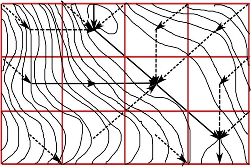
where V_t (m³) is the water storage, ∑q_n (m³/s) is the sum of the net material stream, q^i,j_out (m³/s) is the outflow discharge and K (s⁻¹) is the storage coefficient (Szabó 2007).

The calculation of the DIWA model can be divided into three parts: calculation of the state variables (e.g. interception, evaporation, snow accumulation/melt), the solution of the rainfall–runoff system (percolation, the horizontal components of runoff, interactions between soil layers) and the calculation of runoff in stream channels.

Calibration of the DIWA model to the target area is based on a 2-year period (1 May 2000‒30 April 2002), which includes an extreme flood event (2001) and also periods with lower river discharge values (detailed description can be found in Kis et al. 2017b). The CARPATCLIM-driven simulated values are fitted to the observed river discharge values by adjusting manually some parameters of the model (e.g. the critical temperature of the snowmelt model, the maximum storage capacity of the O-horizon or the vegetation surface, the degree-day factor, the saturated hydraulic conductivity of the O-horizon). The linear correlation value is 0.65, the average difference between the observed and simulated values is 33 m³/s, the RMSE (root mean square error) is 169 m³/s, the Nash-Sutcliffe model efficiency coefficient is 0.6 and the PBIAS (percent bias) is 5.1%.

Methods

Hydrological processes in a well-defined river basin are clearly determined by the actual meteorological situation as the boundary conditions of complex processes. The distributions of long-series meteorological conditions form the climatic factors of a given area, which contribute to the very complex system of global climate. Due to the complexity of the global climate system, it is impossible to provide a perfect meteorological projection for the future, neither on the global scale, nor on a finer, regional scale. An appropriate projection should include an uncertainty evaluation, which is highly recommended in the case of impact studies, so decision-makers can take more responsible actions considering possible consequences (Kundewicz et al. 2016). In addition, hydrological processes involve other factors besides meteorological conditions; therefore, climate model simulations by themselves are not sufficient to provide reliable hydrological estimations and a well-established, integrated approach is needed instead.

Validation results show that the RegCM4 model, like most climate simulations (Kotlarski et al. 2014, Torma 2019), underestimates temperature and precipitation values of the historical time period in some months, while overestimating these values in others (Pieczka et al. 2017, 2018, 2019). Namely, for Hungary, the RegCM4 model overestimates the annual mean temperature by ~0.7°C. Summer temperature is overestimated by more than 2.5°C, while in the other three seasons the temperature bias is less than 1°C (Pieczka et al. 2018). Considering precipitation, the modelled mean annual sum is close to the reference value. However, on a seasonal scale, there are some discrepancies, e.g. in winter and autumn there is overestimation, while in summer and spring underestimation can be found. The spatial distribution of both temperature and precipitation is similar to the reference values (Pieczka et al. 2019). In order to eliminate these systematic errors, a bias-correction method is applied to the raw simulation data in this study. The majority of the bias-correction methods consider only one reference (which is usually based on observations), so climate simulations are fitted to the distribution of this single time series. However, we know that several realizations are possible within the global or regional climate, and the observed meteorological conditions (which are considered as reference) represent only one potential realization, not all of them. Consequently, we should consider our reference data as a sample from a statistical population. This study uses SWGs, i.e. statistical models, for generating stochastic meteorological time series with statistical characteristics similar to the current reality (Maraun et al. 2010). Their advantages include the bias correction of raw climate model outputs (Hall et al. 2014). Furthermore, since runoff is a complex, nonlinear hydrological process, in which even a small change in one factor may result in substantial differences in the final results, numerous possible scenarios of the meteorological variables should be used in order to assess the statistical characteristics. A stochastic weather generator (DIWA-SWG) was used to obtain several, identically probable time series and to determine the statistical properties of the population, whereby a large number of 100-year time series was generated, embedded in an MC cycle. The number of MC cycles was at least 100, and an additional criterion was used to terminate the built-in algorithm. More specifically, the algorithm finishes in cycle k, if the change of the mean and variance of the parameters of the k‒1 generated distributions and the k distribution is less than 10^‒2. The DIWA-SWG was developed by HYDROInform Ltd. (2012), for which the statistical parameters of temperature, dry spells, wet spells and precipitation total are needed.

The DIWA-SWG uses a sine function for modelling daily mean temperature:

(11) $f\left(t\right)=a\cdot sin\left[\left(t-b\right)\cdot \frac{2\pi }{365}\right]+c$(11)

where t (°C) is temperature, a is a multiplicative scale factor, b is a parameter regarding the time-axis, and c is a parameter regarding the y-axis.

For precipitation and the duration of wet and dry spells (a wet spell is defined on a contiguous area with a spatial extent of at least 100 km, and with a minimum of 1 mm daily total precipitation) gamma distributions were fitted:

(12) $f\left(x\right)=\frac{{\lambda }^{\kappa }{x}^{\kappa -1}{\mathrm{e}}^{-\lambda x}}{\mathrm{\Gamma }\left(\kappa \right)}$(12)

where x is the precipitation-related variable, and κ and λ are parameters of the gamma distribution.

The CARPATCLIM data and raw RegCM4 simulation outputs were obtained for one historical and two future time periods: 1972‒2001, 2021‒2050, 2069‒2098. Assuming that the statistical characteristics of bias will remain the same in the future, the parameters of Eqs. (11)(11) $f\left(t\right)=a\cdot sin\left[\left(t-b\right)\cdot \frac{2\pi }{365}\right]+c$(11) and (12)(12) $f\left(x\right)=\frac{{\lambda }^{\kappa }{x}^{\kappa -1}{\mathrm{e}}^{-\lambda x}}{\mathrm{\Gamma }\left(\kappa \right)}$(12) distributions for future periods were adjusted according to the difference between the CARPATCLIM data and the RegCM4 simulation outputs in the historical time period for each month separately.

The validation of the bias-corrected RegCM4 simulation is presented in Fig. 3 based on the monthly mean temperature values and precipitation sums in the period 1972‒2001. They do not match perfectly, as CARPATCLIM provides only one realization of the possible climate conditions, while the bias-corrected RegCM4 in Fig. 3 gives the average of the possible climate realizations provided by the WG embedded in an MC cycle. However, we can conclude that the annual distribution of both temperature and precipitation is reliable; furthermore, the differences are less than 1.5°C in the case of temperature and less than 11 mm in the case of precipitation. The DIWA hydrological model was driven by all these above-mentioned time series; hence, several hundreds of scenarios with equal theoretical probability can be evaluated for the historical and the two future time periods. The validation results were satisfactory (Kis et al. 2017b), so the proposed model system can be considered as an adequate tool to analyse the possible impacts of climate change on runoff.

Figure 3. Monthly mean temperature and precipitation sum in the period 1972‒2001 based on the CARPATCLIM database (dark grey) and the mean of the bias-corrected RegCM4 simulations provided by a WG embedded in MC cycle (light grey).

Target area

This study analysed the Upper Tisza catchment (~9707 km²), located in eastern Central Europe (see Fig. 4). It is a part of the catchment of the second-longest river in Europe, the River Danube. The Upper Tisza basin is shared by three countries: Ukraine, Romania and Hungary.

Figure 4. Location of the target area: the Upper Tisza catchment (red). Tiszabecs, the cross-section of the River Tisza where it enters Hungary, is indicated by the blue dot.

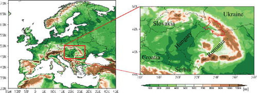
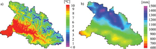
The area has quite a complex topography: there are mountains above 2200 m a.s.l. and lowlands less than 400 m a.s.l.; the average height is 800‒900 m a.s.l. The gradient is steeper than 0.1 m/m in ~30% of the basin, and it can reach 0.33 m/m.

Topography clearly has an effect on climatic conditions: in the mountainous regions, the yearly average temperature is 3‒6°C, while in the lowlands it is 8‒10°C (Fig. 5(a)) based on CARPATCLIM data, 1972‒2001. Considering the spatial averages in the catchment, the mean annual temperature is 6.1°C; the maximum of monthly means is in July (15.8°C), the minimum is in January (‒4.4°C). In the investigated historical time period, the warmest year was 1994 (7.5°C), while the coldest was 1980 (5.0°C). The total annual precipitation is 1200 and 900 mm/year at the higher and lower elevations, respectively, on average (Fig. 5(b)); the spatial mean is 1075 mm (but individual years can differ substantially, of course). The wettest months are June and July (~130 mm/month) and the driest is February (54 mm/month). There were two particularly wet years in the 1972‒2001 reference period: 1998 and 2001, with a sum of annual precipitation of more than 1400 mm. The driest year was 1990, with an annual total of less than 900 mm.

Figure 5. (a) Mean annual temperature and (b) precipitation sum in the Upper Tisza catchment, based on CARPATCLIM data, 1972‒2001.

Considering the land use, most of the domain is covered by broad-leaved and coniferous forests, displaying a substantial water-retention effect, but there are also non-irrigated arable lands, mixed forests, natural grasslands and pastures where a greater amount of runoff occurs. Infiltration capacity strongly depends on soil type, as the porosity of the soil plays a key role in water storage capacity and in the resistance of water to flow into deeper layers. Sand has quite high infiltration capacity, while for loam and clay it is smaller. In the target domain, most of the soil is sandy loam; in the southern parts sand (east), clay loam (central) and loam (west along the Tisza) can be found. The spatial distribution of land use and soil types in the Upper Tisza Basin is given in Kis et al. (2017b). Detailed information about the characteristics of the land-use types occurring in the target area are presented in Table 2.

Table 2. Main characteristics of the Upper Tisza Basin for different land-use types.

Land-use type	LAI max	pF max	O-horizon max (mm)	Root depth max (mm)	Surface storage capacity max (mm)	Saturated hydrological conductivity (m d^−1)
Broad leaved forest	7	4.2	85	1500	30	600
Coniferous forest	45	4.2	70	1500	20	500
Non-irrigated arable land	4.5	3.8	15	400	50	500
Mixed forests	12	4.2	100	1500	25	500
Pastures	1.5	3.8	30	300	15	900
Natural grassland	6	3.8	20	300	10	800
Transitional woodland-scrub	5	3.8	40	500	15	1200
Mix agriculture and natural vegetation	6	3.8	10	500	20	800

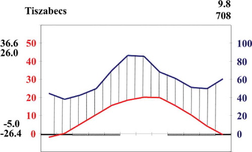
In the following, our results are presented for the Tiszabecs gauging stage, where the Tisza enters Hungary. The average daily flow rate was 212 m³/s at this station in the period 1960‒2003, according to the observations. The maximum value of about 4600 m³/s occurred in March 2001, the minimum (11 m³/s) in August 1994. On average, the largest flow rate values are found in spring, when snow melting plays a key role. The smallest values occur between August and October, which can be explained by the low precipitation amount and enhanced late-summer evapotranspiration. A Water-Lieth diagram (Walter and Lieth 1960) is presented in Fig. 6 based on CARPATCLIM data for 1972‒2001 to characterize the climate conditions of Tiszabecs. The highest temperature values occur in summer, while the lowest are found in winter; the yearly average is 9.8°C. The coldest month is January (with 1.9°C monthly average), the hottest is July (with 20.3°C monthly average). In the investigated time period, the absolute range of temperature is quite high: the minimum is ‒26.4°C and the maximum 36.6°C. The wettest season is summer (~85 mm/month); the driest period is in late-winter and early-spring (~40 mm/month).

Figure 6. Walter-Lieth climate diagram for Tiszabecs (48.1°N, 22.8°E) based on CARPATCLIM data, 1972‒2001.

Results and discussion

First, a brief overview of the projected climate change in the Upper Tisza basin is presented. Then, the distribution of runoff and extreme characteristics is analysed on annual and monthly scales for Tiszabecs based on the several hundred, equally probable, 100-year simulations (provided by the MC cycle). Three time periods are investigated, namely, the historical (1972‒2001), the near future (2021‒2050) and the end of the 21st century (2069‒2098).

Climate change in the Upper Tisza catchment

According to our climate simulations, warmer conditions are likely to occur in the target domain. The estimated increase for 2021‒2050 is 1‒1.5°C in winter and 3°C in summer; by the end of the 21st century, this equates to more than 3.5°C in every season. Based on our results, the mean temperature in the coldest month (January) will be 0.3°C (so there will not be any month when the average temperature is below 0°C, according to the mean of the simulations). Considering precipitation, the largest changes are estimated for summer, when a clear decreasing trend is likely to occur, especially in July and August, when it may exceed 40% by the end of the 21st century. A decreasing tendency is also projected for September and October, while from November to April a slight increase is estimated.

Estimated runoff characteristics for the Tiszabecs gauging station

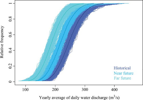
In accordance with the projected temperature and precipitation changes, runoff is estimated to decrease on the annual scale. In Fig. 7 distribution of runoff is presented for the three time periods (thin lines show the individual simulations, thicker lines refer to their mean). The projected changes for the near future are smaller, some simulations even show an increase, but the average is clearly likely to decrease (by 12% in the case of the 50th percentile). By the end of the 21st century, the changes are more pronounced (24% on average in the case of the 50th percentile).

Figure 7. Distribution of the yearly average of daily water discharge in the three investigated time periods based on DIWA-HFMS outputs driven by meteorological time series generated by the DIWA-SWG embedded in an MC cycle. Individual simulations are marked with thin lines; thicker, darker lines show their average.

Comparing the three investigated time periods based on some statistical characteristics of the simulations, it can be seen that the 10th percentile value shows a greater decrease in April, July, August and September (almost gradually for the near and the far future) as well as in the case of the 90th percentile (Fig. 8(a)). The difference between the modus and median is generally greater in the historical time period than in the future time slices, which indirectly implies the decrease of asymmetry in the frequency distribution of river discharge. The standard deviation of the simulations within the MC cycle is generally decreasing, especially in July, August and September, which implies a decrease of the uncertainty of projections.

Figure 8. (a) The averages of major statistical values (minimum, maximum, 10th, 50th and 90th percentiles) of river discharge in the historical and future time periods on a monthly scale and (b) the average relative change (%) of the daily mean discharge values for the near and far future based on DIWA-HFMS outputs driven by meteorological time series generated by the DIWA-SWG embedded in an MC cycle for Tiszabecs.

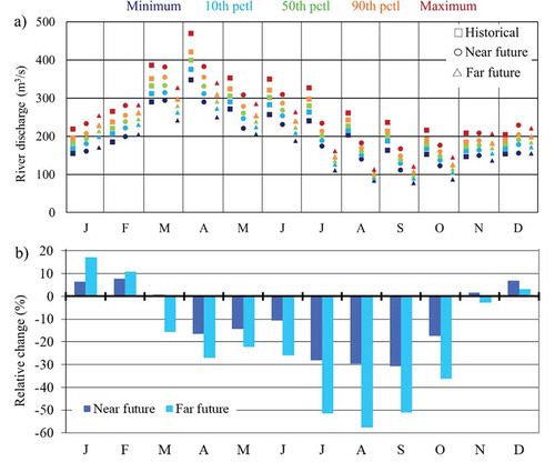
If we consider the relative changes in runoff values on a monthly scale, the changes are more pronounced in the far future in most months (Fig. 8(b)). It can also be concluded that in most cases a decreasing trend of river discharge is likely to occur; however, in January and February, a slight increase is estimated for the future time periods. In the historical time period, the lower values occurred in winter and autumn. Winter is the driest season in the target area and also the coldest, so the proportion of snow is higher, which can accumulate and contribute to the runoff later. Therefore, it is quite understandable why the lowest values occur in this season. At the same time, it is interesting to note that the only increasing trend is projected for winter, which is less than 20%, on average. This is a possible consequence of the projected climate change: precipitation is likely to increase in winter; furthermore, temperatures are estimated to be higher, so the proportion of snow (and the accumulated snowpack within the winter season) will decrease. Hence, less snow is expected to accumulate, so precipitation in these months can enter the river directly, resulting in relatively higher runoff values and stream water levels.

The highest values can be seen in spring: 300‒400 m³/s in the historical time period, yet 200‒300 m³/s by the end of the 21st century (Fig. 8(a)). At the same time, the highest uncertainty also occurs in this season. The decreasing tendency in spring (especially in April) can be related to the lack of snow, as in winter less snow is projected to accumulate, evidently less snow will melt and flow into the river as the weather gets warmer. Hence, compared to the historical time period, runoff will decrease in this season. Even so, higher runoff values within a year are projected for the spring by the end of the 21st century, with only the estimated runoff in February being close to them. For the Czech Republic, Hanel et al. (2012) obtained similar results for spring and they concluded that further investigations are needed in order to plan the construction of water reservoirs at appropriate locations. It would be important to use the collected winter surplus later in summer.

The largest relative changes are projected for summer: in the near future the mean decrease is ~30%, while in the far future it is ~60% in August, and ~50% in July and September (Fig. 8(b)). This trend may occur due to the overall drying in this season (Kis et al. 2017a). Furthermore, higher temperatures can enhance potential evaporation as well, which can foster a decrease in runoff. As a result, the lowest runoff values are projected for late summer and early autumn months by the end of the 21st century, unlike in the historical time period when these occurred in late autumn and winter (Fig. 8(a)). The selected percentile values (i.e. 10th, 50th, 90th percentiles) are the closest to each other in August in the far future (the total range encompasses 29 m³/s), so the uncertainty of the projected changes is the smallest within the year, thus a decreasing trend is quite likely to occur in this month. From July to October, the differences between the simulations are also quite small, with the total range of values less than 60 m³/s.

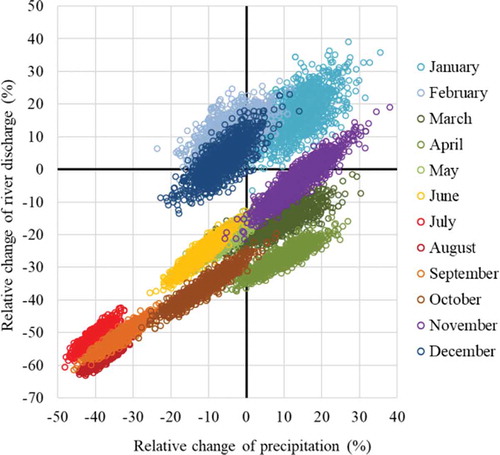
In general, the projected change of precipitation causes similar change in river discharge, as shown in Fig. 9. However, we can also conclude that even if precipitation will increase in certain months, a decrease in river discharge may occur – for example, in March and April. This can be probably explained by the consequence of overall warming, namely, less snow and more rain are likely to occur; therefore, a snowmelt-induced surplus of river discharge in spring will not occur in the future. This effect is greater than the small increase in precipitation (<0‒25%). On the contrary, according to the majority of simulations, a decreasing trend in precipitation is estimated in December and February; however, river discharge is projected to increase. This is also related to snow, as the proportion of rain will increase in winter because of higher temperatures, and this plays a greater role in river discharge than the projected precipitation changes, according to our results.

Figure 9. Monthly relative changes of precipitation and river discharge in the far future based on the WG generated precipitation series and DIWA simulations embedded in an MC cycle. The monthly averages of the simulations in the historical time period served as the reference.

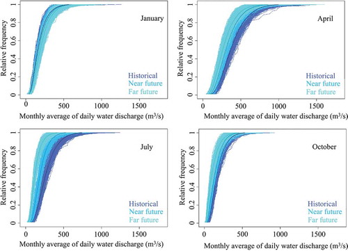
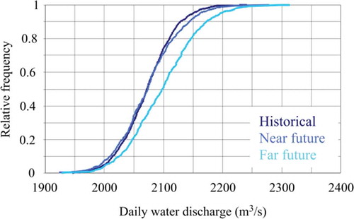
Considering the distribution functions for each month, the projected changes by the end of the 21st century are significant from April to October, according to the Kolmogorov–Smirnov test (Kolmogorov 1933). The distribution of daily discharge for the middle month of each season is presented in Fig. 10. In January, a slight increase in runoff is likely to occur, but there is quite a large overlap between the ranges of the simulations in the three time periods. In April, the near future is closer to the historical time period, and, evidently, a decreasing tendency is projected for the far future. In July, a gradual decrease can be seen: the sets of simulations of the three time periods can be clearly distinguished. It can also be concluded that the higher the percentile value, the greater the change and spread of the simulations. For October, smaller changes are projected. The overlap between the simulation ensembles in the different time periods is similar to January, but the sign of the change is the opposite.

Figure 10. Distribution of the monthly (January, April, July, October) average of daily discharge in the three selected time periods based on DIWA-HFMS outputs driven by meteorological time series generated by the DIWA-SWG embedded in an MC cycle for Tiszabecs. Individual simulations are marked with thin lines; thicker, darker lines show their average.

In our previous study (Kis et al. 2017b), a simpler method was applied to the analysis (without uncertainty ranges); however, the projected changes in seasonal runoff were similar (i.e. summer decrease and winter increase). Radvánszky and Jacob (2008) also focused on the effects of climate change on the Tisza; they used climatological and hydrological models that are different from the models applied to the present study (namely, the REMO regional climate model, Jacob and Podzun 1997 and the HD hydrological model, Hagemann and Dümenil 1998). Nevertheless, they concluded similar results: a decrease in summer and autumn runoff is likely to occur in the future. Didovets et al. (2019) used both the RCP4.5 and RCP8.5 emissions scenarios in their investigation considering the Prut and Tisza catchments in Ukraine. In the case of RCP4.5, an increase in the 30-year flood level is projected, while for RCP8.5, uncertainty was quite high with changes in both directions.

Estimated extreme characteristics for Tiszabecs

In this study, extreme characteristics of runoff are also investigated (both high and critically low values).

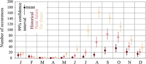
First, we analysed the critical low water level. For this, we calculated the mean of the annual minimum values based on historical data for the past 100 years, which turned out to be 110 m³/s. After this, for each time period, we determined how many times and for how long (within 100 years) the discharge was below or equal to this threshold. It can be clearly seen that increases in the occurrence of critical low water levels are projected in most of the months (Fig. 11). This will be particularly robust in late summer to early autumn. Low water levels occurred the most frequently in October in the historical time period. This will shift to September by the middle of the 21st century, according to our simulations (however, considering the 99% confidence interval, there is only a slight difference between the two autumn months). Then, the most occurrences of a critical low water level will take place in August, on average, in the late-century period. From June to December, a larger increase is estimated compared to the rest of the year. According to our simulations, the spring minimum will not change during the 21st century.

Figure 11. Total number of days below the critical low water level in 100 years in the three investigated time periods based on DIWA-HFMS outputs driven by meteorological time series generated by the DIWA-SWG embedded in an MC cycle for Tiszabecs.

The analysis continues with high-water levels, represented here by the investigation of level-3 flood warnings at the Tiszabecs gauging station. A level-3 flood warning is issued for this stage if the water level exceeds 500 cm.⁶ According to our simulations, the total number of level-3 flood warnings will decrease by 30% and 40% annually, on average, by the middle and late century, respectively (Fig. 12). More specifically, a level-3 flood warning occurred 52 times on average in 100 years within the historical time period. By the middle of the 21st century level-3 flood warnings are estimated to occur only 37 times, and by the end of the 21st century only 31 times. To conclude, while the water level was higher than 500 cm in every second year in the historical time period, it will occur only in every third year, on average, in the far future.

Figure 12. Number of days in excess of the level-3 flood warning in 100 years in the three investigated time periods based on DIWA-HFMS outputs driven by meteorological time series generated by the DIWA-SWG embedded in an MC cycle for Tiszabecs.

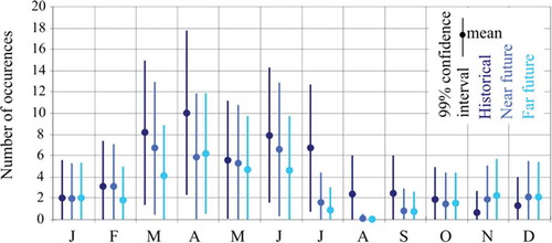
Level-3 flood warnings occurred most often from March to July in the historical time period (6‒10 events/month in 100 years, on average; but the confidence interval is quite wide: ranging from 2 to 18 events/month). The reason for such intra-annual distribution is clearly a consequence of general meteorological conditions; more specifically, spring floods are related to snow melting, while summer floods stem from higher precipitation due to frontal activity and more intense convective processes. The most frequent occurrence is likely to remain in the period from March to June in the future; however, the future average occurrence is projected to decrease to 4‒6 events/month. Fewer spring floods are likely to occur in Scandinavia in the future for similar reasons (EEA 2016). According to Dankers and Feyen (2008) fewer floods are expected in Central and Southern Europe, too.

The least number of level-3 flood warnings was detected in November and December in the historical time period. An increasing trend is estimated in these months according to the simulations; hence, the lowest frequency is expected to shift to late summer and early autumn (July, August, September) in the future.

All the above implies that, overall, the number of level-3 flood warnings is estimated to decrease in the 21st century. A decrease of 50‒60% (on average) is projected for March and April, as the snow-related floods will occur less often due to the projected lack of snow as a direct consequence of regional warming. The greatest changes (i.e. 90‒100%, on average) are simulated for July, August and September. For instance, according to our results, no level-3 flood warning will occur in August in the late 21st century. This substantial decrease can be related to the general summer drying trend: as a result of less precipitation and longer mean dry spells, rivers are likely to have lower water levels. Therefore, when wet periods occur with high precipitation towards the end of the 21st century, they will not result in such extreme high-water levels as in the historical time period.

Besides the analysis of the monthly number of occurrences, the daily average water discharge values are also calculated in the case of the level-3 flood warnings. We compared their distribution in the three time periods (Fig. 13). The distribution function in the near future is quite similar to that of the historical period. However, substantially greater changes are projected for the end of the 21st century, especially in the case of higher percentile values. Although fewer events will tend to exceed the level-3 flood warning in the future, flood levels are nevertheless generally projected to become more severe than nowadays in certain cases. Similar results are projected by Christensen and Christensen (2003), namely, a trend towards more severe floods in the late century compared to the recent past.

Figure 13. Distribution of daily water discharge in excess of the level-3 flood warning in the three investigated time periods based on DIWA-HFMS outputs driven by meteorological time series generated by the DIWA-SWG embedded in an MC cycle for Tiszabecs.

In Switzerland, a decrease in discharge will likely to occur in August and September, according to the analyses of Fatichi et al. (2015). In Austria, in the Ötztal Alps, a decrease in annual runoff is estimated (Hanzer et al. 2018, Strasser et al. 2019). The increase in winter and the decrease in summer and spring is expected to occur in several catchments in the Czech Republic (Hanel et al. 2012). However, in Poland, an increase in flood indices is estimated (Osuch et al. 2017) in the northern areas, where overall precipitation increase is likely to occur according to the climate simulations. Moreover, earlier spring floods are expected in Ukraine (Didovets et al. 2017). In Slovakia, which is quite close to our target area, an increase in extreme floods is likely to occur in the future, too (Kohnová et al. 2019). Overall, the results of our analyses are in a good agreement with the above hydrological studies conducted in neighbouring countries.

Our results highlight the importance of properly managing and supplying both technical equipment and human resources for flood control; furthermore, healthcare and social services should also be prepared in case of evacuation or epidemic diseases due to floods. The interviews of Vari et al. (2003) concluded that the most severe consequences of floods in Hungary include damage to homes, properties and roads, the impossibility of farming activities, illness and pollution spreading by floodwaters. It is necessary to preserve (e.g. prevent leakage in dykes, dredge river beds, not build in the flood basin) and to improve (e.g. develop dyke systems, elevate dams, remove buildings from the flood basin, optimize plant cultivation/land use, construct reservoirs) currently existing protective capacity taking into account local circumstances. Emergency reservoirs can also be useful tools to support flood-defence systems, as they can reduce the flood peak by redirecting the water to a non-inundated, agricultural or forest area selected in advance. Built or designated storage basins can serve as appropriate solutions too, since they are suitable for seasonal storage (Szentiványi 2015), which is important in the light of our results (more critically low water levels and fewer, but occasionally more severe, floods).

Conclusions

The potential effect of climate change on runoff is analysed in this study for the Upper Tisza catchment. The topicality of this issue is that climate change does not only mean higher temperature values, but a possible redistribution of precipitation in time and the occurrence of more frequent extreme events as well, which may result in damage in different sectors.

For the investigation, we applied the combined use of a coherent set of advanced numerical models, which were able to produce the runoff characteristics under both the present (based on CARPATCLIM database) and the future (based on RegCM4 model output data) climate conditions.

According to our results for the Tiszabecs gauging station, the daily mean discharge will decrease in the 21st century, especially in summer. The changes are significant from April to October, according to the Kolmogorov–Smirnov test. For winter, a slight increase is projected. The number of days with a critical low water level is projected to increase in the future in every month from July to October, in particular by the end of the 21st century. On the other hand, the number of days in excess of the level-3 flood warning is projected to decrease in the future. Spring floods are estimated to occur less frequently due to higher temperatures and, thus, fewer snowfall events, resulting in less snow to accumulate and melt. The frequency of summer floods is likely to decrease because of the projected drying tendency (i.e. less precipitation and longer dry spells). It is important to note that although the total number of days in excess of the level-3 flood warning is estimated to decrease, the maximum values of 100-year flood levels are projected to be greater in certain cases compared to the historical time period. Thus, adaptation strategies should take into account the above-mentioned climate change trends and include both flood-defence efforts and proper water storage plans to provide sufficient water for different users.

We note that, besides the effects of climate change, land-use change may also affect hydrological processes. On the one hand, Hejazi and Moglen (2008) found that climate change plays a greater role in influencing flow durations than land-use changes. On the other hand, other studies (e.g. Marhaento et al. 2018) concluded that land use is an appropriate tool to mitigate water-related hazards. In the present study, however, any other factor (beyond climate change) that can contribute to the modification of hydrological processes (e.g. land use, river regulation, dredging, morphological properties of the catchment) is assumed to be unchanged. Nevertheless, it is interesting to note that, according to the research of Vari et al. (2003), stakeholders claimed that flood risk is increasing in our target area due to technical deficiencies, land-use changes (mainly deforestation) and lack of mitigation; global climate change was not mentioned as a direct reason for the increase. This implies a potential continuation of the study to focus on land-use changes in addition to the effects of climate change.

Disclosure statement

No potential conflict of interest was reported by the authors.

Additional information

Funding

Research leading to this paper was supported by the following sources: the Széchenyi 2020 program, the European Regional Development Fund and the Hungarian Government via the AgroMo project (grant number: GINOP-2.3.2-15-2016-00028), the Hungarian National Research, Development and Innovation Fund under grants K-129162 and K-120605, and the Hungarian Ministry of Human Capacities under the ELTE Excellence Program (grant number: 783-3/2018/FEKUTSRAT). The CARPATCLIM Database used in this study was compiled with the support of the European Commission in JRC in 2013.

Notes

¹ http://ec.europa.eu/environment/water/flood_risk/index.htm.

² https://www.medcordex.eu/index.php/.

³ https://land.copernicus.eu/pan-european/corine-land-cover/clc-2012.

⁴ https://data.jrc.ec.europa.eu/dataset/jrc-mappe-europe-setup-d-18-lai/resource/8945dbfa-d9ce-4e96-880c-06f32d506bae.

⁵ https://esdac.jrc.ec.europa.eu/resource-type/datasets?fbclid=IwAR0flWqWBiBsmPpSZ5bKVFMZd-IM4LNxf4e05eTEcCZOI3Iq4xvTvqJyJ3k.

⁶ https://www.vizugy.hu/?mapModule=OpGrafikon&AllomasVOA=16496327-97AB-11D4-BB62-00508BA24287&mapData=Idosor#mapData.

References

- Addor, N. and Seibert, J., 2014. Bias correction for hydrological impact studies – beyond the daily perspective. Hydrological Processes, 28, 4823–4828. doi:10.1002/hyp.10238
- Ahmed, S. and Tsanis, I., 2016. Watershed response to bias-corrected improved skilled precipitation and temperature under future climate – a case study on Spencer Creek Watershed, Ontario, Canada. Hydrology Current Research, 7, 246. doi:10.4172/2157-7587.1000246
- Alfaro, S.C. and Gomes, L., 2001. Modeling mineral aerosol production by wind erosion: emission intensities and aerosol size distributions in source areas. Journal of Geophysical Research, 106, d16. doi:10.1029/2000JD900339
- Amani, A. and Lebel, T., 1997. Lagrangian kriging for the estimation of Sahelian rainfall at small time steps. Journal of Hydrology, 192, 125‒157. doi:10.1016/S0022-1694(96)03104-6
- Andrej, C. and Kajfez-Bogataj, L., 2012. Simulation of maize yield in current and changed climatic conditions: addressing modelling uncertainties and the importance of bias correction in climate model simulations. European Journal of Agronomy, 37 (1), 83‒95.
- Annis, A., et al., 2020. Quantifying the relative impact of hydrological and hydraulic modelling parameterizations on uncertainty of inundation maps. Hydrological Sciences Journal, 65, 507‒523. doi:10.1080/02626667.2019.1709640
- Becker, A., et al., 2018. Implications of climate change for shipping: ports and supply chains. WIREs Climate Change, 9, e508. doi:10.1002/wcc.508
- Bisselink, B., et al., 2018. Impact of a changing climate, land use, and water usage on water resources int he Danube river basin. Luxembourg: Publications Office of the European Union, EUR 29228 EN, ISBN 978-92-79-85889-5. doi:10.2760/89828/JRC111817
- Blöschl, G., et al., 2017. Changing climate shifts timing of European floods. Science, 357 (6351), 588‒590. doi:10.1126/science.aan2506
- Cameron, D., Beven, K., and Naden, P., 2000. Flood frequency estimation by continuous simulation under climate change (with uncertainty). Hydrology and Earth System Sciences, 4 (3), 393–405. doi:10.5194/hess-4-393-2000
- Challinor, A.J., et al., 2018. Improving the use of crop models for risk assessment and climate change adaptation. Agricultural Systems, 159, 296–306. doi:10.1016/j.agsy.2017.07.010
- Charalambous, J., Rahman, A., and Carroll, D., 2013. Application of Monte Carlo simulation technique to design flood estimation: a case study for North Johnstone River in Queensland, Australia. Water Resources Management, 27, 4099–4111. doi:10.1007/s11269-013-0398-9
- Chen, J., et al., 2017. Impacts of weighting climate models for hydro-meteorological climate change studies. Journal of Hydrology, 549, 534–546. doi:10.1016/j.jhydrol.2017.04.025
- Chen, J., Brissette, F.P., and Leconte, R., 2011. Uncertainty of downscaling method in quantifying the impact of climate change on hydrology. Journal of Hydrology, 401, 190–202. doi:10.1016/j.jhydrol.2011.02.020
- Christensen, J.H. and Christensen, O.B., 2003. Climate modelling: severe summertime flooding in Europe. Nature, 421, 805–806. doi:10.1038/421805a
- Clark, M.P., et al., 2016. Characterizing uncertainty of the hydrologic impacts of climate change. Current Climate Change Reports, 2, 55–64. doi:10.1007/s40641-016-0034-x
- Collins, W.J., et al., 2011. Development and evaluation of an earth-system model – Hadgem2. Geoscientific Model Development Discussions, 4, 997–1062. doi:10.5194/gmdd-4-997-2011
- Cressie, N.A.C., 1985. Fitting variogram models by weighted least squares. Journal of the International Association for Mathematical Geology, 17, 563‒586. doi:10.1007/BF01032109
- Dankers, R. and Feyen, L., 2008. Climate change impact on flood hazard in Europe: an assessment based on high-resolution climate simulations. Journal of Geophysical Research, 113, D19105. doi:10.1029/2007JD009719
- Darcy, H., 1856. Les fontaines publiques de la ville de Dijon. Paris: Dalmont, 647.
- Depla, I., et al., 2009. Impacts of climate change on surface water quality in relation to drinking water production. Environment International, 35 (8), 1225–1233. doi:10.1016/j.envint.2009.07.001
- Diaz-Ramirez, J., et al., 2012. Parameter uncertainty methods in evaluating a lumped hydrological model. Obras y Proyectos, 12, 42‒56.
- Dickinson, R.E., Henderson-Sellers, A., and Kennedy, P.J., 1993. Biosphere-atmosphere transfer scheme (BATS) Version 1e as coupled to the NCAR community climate model. NCAR Technical Note NCAR/TN-387 + STR. doi: 10.5065/D67W6959
- Didovets, I., et al., 2017. Assessment of climate change impacts on water resources in three representative Ukrainian catchments using eco-hydrological modelling. Water, 9, 204. doi:10.3390/w9030204
- Didovets, I., et al., 2019. Climate change impact on regional floods in the Carpathian region. Journal of Hydrology: Regional Studies, 22, 100590. doi:10.1016/j.ejrh.2019.01.002
- Dirks, J.A., et al., 2015. Impacts of climate change on energy consumption and peak demand in buildings: a detailed regional approach. Energy, 79, 20‒32. doi:10.1016/j.energy.2014.08.081
- EC (European Commission), 2019. Report from the commission to the European Parliament and the council on the implementation of the Water Framework Directive (200/60/EC) and the Floods Directive (2007/60/EC) Second River Basin Management Plans First Flood Risk Management Plans. Brussels, 26 February.
- EEA (European Environment Agency), 2016. Flood risks and environmental vulnerability. European Environment Agency Report no. 1/2016. ISSN: 1977‒8449.
- Ehret, U., et al., 2012. HESS Opinions: “Should we apply bias correction to global and regional climate model data?”. Hydrology and Earth System Sciences, 16, 3391–3404. doi:10.5194/hess-16-3391-2012
- Eisner, S., et al., 2017. An ensembles analysis of climate change impacts on streamflow seasonality across 11 large river basins. Climatic Change, 141 (3), 401–417. doi:10.1007/s10584-016-1844-5
- Elguindi, N., et al., 2011. Regional climatic model RegCM – user manual. Version 4.3. Trieste, Italy: ICTP, 32.
- Emanuel, K.A., 1991. A scheme for representing cumulus convection in large-scale models. Journal of the Atmospheric Sciences, 48 (21), 2313–2335. doi:10.1175/1520-0469(1991)048<2313:ASFRCC>2.0.CO;2
- Evans, G.W., 2019. Projected behavioral impacts of global cliamte change. Annual Review of Psychology, 70, 449–474. doi:10.1146/annurev-psych-010418-103023
- Fatichi, S., et al., 2015. High-resolution distributed analysis of climate and anthropogenic changes on the hydrology of an Alpine catchment. Journal of Hydrology, 525, 362–382. doi:10.1016/j.jhydrol.2015.03.036
- Filho, W.L., et al., 2018. Strengthening climate change adaptation capacity in Africa – case studies from six major African cities and policy implications. Environmental Science & Policy, 86, 29–37. doi:10.1016/j.envsci.2018.05.004
- Fritsch, J.M. and Chappell, C.F., 1980. Numerical prediction of convectively driven mesoscale pressure systems. Part I: convective parameterization. Journal of the Atmospheric Sciences, 37, 722–1733.
- Garner, G., et al., 2015. Hydroclimatology of extreme river flows. Freshwater Biology, 60, 2461‒2476. doi:10.1111/fwb.12667
- Giuntoli, I., et al., 2015. Future hydrological extremes: the uncertainty from multiple global climate and global hydrological models. Earth System Dynamics, 6, 267–285. doi:10.5194/esd-6-267-2015
- Gosling, S.N. and Arnell, N.W., 2016. A global assessment of the impact of climate change on water scarcity. Climatic Change, 134 (3), 371–385. doi:10.1007/s10584-013-0853-x
- Grell, G.A., 1993. Prognostic evaluation of assumptions used by cumulus parameterizations. Monthly Weather Review, 121 (3), 764–787. doi:10.1175/1520-0493(1993)121<0764:PEOAUB>2.0.CO;2
- Hagemann, S., et al., 2011. Impact of a statistical bias correction on the projected hydrological changes obtained from three GCMs and two hydrology models. Journal of Hydrometeorology, 12, 556–578. doi:10.1175/2011JHM1336.1
- Hagemann, S. and Dümenil, L., 1998. A parameterization of the lateral waterflow for the global scale. Climate Dynamic, 14 (1), 17–31. doi:10.1007/s003820050205
- Hall, J., et al., 2014. Understanding flood regime changes in Europe: a state-of-theart assessment. Hydrology and Earth System Sciences, 18, 2735‒2772. doi:10.5194/hess-18-2735-2014
- Hanel, M., et al., 2012. A multi-model assessment of climate change impact on hydrological regime in the Czech Republic. Journal of Hydrology and Hydromechanics, 60 (3), 152–161. doi:10.2478/v10098-012-0013-4
- Hansen, G. and Cramer, W., 2015. Global distribution of observed climate change impacts. Nature Climate Change, 5, 182‒185. doi:10.1038/nclimate2529
- Hanzer, F., et al., 2018. Projected cryospheric and hydrological impacts of 21st century climate change in the Ötztal Alps (Austria) simulated using a physically based approach. Hydrology and Earth System Sciences, 22, 1593–1614. doi:10.5194/hess-22-1593-2018
- Hawkins, E. and Sutton, R., 2011. The potential to narrow uncertainty in regional climate predictions. Climate Dynamics, 37, 407–418. doi:10.1007/s00382-010-0810-6
- Hejazi, M.I. and Moglen, G.E., 2008. The effect of climate and land use change on flow duration in Maryland Piedmont region. Hydrological Processes, 22, 4710‒4722. doi:10.1002/hyp.7080
- Hirabayashi, Y., et al., 2013. Global flood risk under climate change. Nature Climate Change, 3, 816–821. doi:10.1038/nclimate1911
- Holtslag, A.A.M., De Bruijn, E.I.F., and Pan, H.L., 1990. A high resolution air mass transformation model for short-range weather forecasting. Monthly Weather Review, 118 (8), 1561–1575. doi:10.1175/1520-0493(1990)118<1561:AHRAMT>2.0.CO;2
- Hostetler, S.W., Bates, G.T., and Giorgi, F., 1993. Interactive nesting of a lake thermal model within a regional climate model for climate change studies. Geophysical Research, 98, 5045–5057. doi:10.1029/92JD02843
- Huang, S., et al., 2013. Projections of climate change impacts on river flood conditions in Germany by combining three different RCMs with a regional eco-hydrological model. Climatic Change, 113 (3‒4), 631‒663. doi:10.1007/s10584-012-0586-2
- Hutchins, M.G., et al., 2016. Projections of future deterioration in UK river quality are hampered by climatic uncertainty under extreme conditions. Hydrological Sciences Journal, 61, 2818‒2833. doi:10.1080/02626667.2016.1177186
- IPCC (Intergovernmental Panel on Climate Change), 2012. In: C.B. Field, et al., eds. Managing the risks of extreme events and disasters to advance climate change adaptation. A special report of working groups I and II of the intergovernmental panel on climate change. Cambridge, UK and New York, NY: Cambridge University Press.
- Jacob, D. and Podzun, R., 1997. Sensitivity studies with the regional climate model REMO. Meteorology and Atmospheric Physics, 63, 119–129. doi:10.1007/BF01025368
- Joseph, J., et al., 2018. Hydrologic impacts of climate change: comparisons between hydrological parameter uncertainty and climate model uncertainty. Journal of Hydrology, 566, 1–22. doi:10.1016/j.jhydrol.2018.08.080
- Karlsson, I.B., et al., 2016. Combined effects of climate models, hydrological model structures and land use scenarios on hydrological impacts of climate change. Journal of Hydrology, 535, 301‒317. doi:10.1016/j.jhydrol.2016.01.069
- Kay, A.L. and Jones, R.G., 2012. Comparison of the use of alternative UKCP09 products for modelling the impacts of climate change on flood frequency. Climatic Change, 114, 211–230. doi:10.1007/s10584-011-0395-z
- Kiehl, J.T., et al., 1996. Description of the NCAR community climate model (CCM3). Tech. Rep. NCAR/TN-420 + STR. Boulder: NCAR.
- Kis, A., et al., 2017b. Application of RCM results to hydrological analysis. Idojárás – Quarterly Journal of the Hungarian Meteorological Service, 121 (4), 437–452.
- Kis, A., Pongrácz, R., and Bartholy, J., 2017a. Multi-model analysis of regional dry and wet conditions for the Carpathian Region. International Journal of Climatology, 37, 4543–4560. doi:10.1002/joc.5104
- Kohnová, S., et al., 2019. Future impacts of land use and climate change on extreme runoff values in selected catchments of Slovakia. Meteorology Hydrology and Water Management, 7 (1), 47‒55. doi:10.26491/mhwm/97254
- Kolmogorov, A.N., 1933. Sulla Determinazione Empirica di Una Legge di Distribuzione. Giornale dell’Istituto Italiano degli Attuari, 4, 83‒91.
- Köplin, N., et al., 2014. Seasonality and magnitude of floods in Switzerland under future climate change. Hydrological Processes, 28 (4), 2567‒2578. doi:10.1002/hyp.9757
- Kotlarski, S., et al., 2014. Regional climate modeling on European scales: a joint standard evaluation of the EURO-CORDEX RCM ensemble. Geoscientific Model Development, 7, 1297–1333. doi:10.5194/gmd-7-1297-2014
- Kour, R., Patel, N., and Krishna, A.P., 2016. Climate and hydrological models to assess the impact of climate change on hydrological regime: a review. Arabian Journal of Geosciences, 9 (544), 31p. doi:10.1007/s12517-016-2561-0
- Kundewicz, Z.W., et al., 2013b. Flood risk and climate change: global and regional perspectives. Hydrological Sciences Journal, 59:1, 1‒28. doi:10.1080/02626667.2013.857411
- Kundewicz, Z.W., et al., 2016. Differences in flood hazard projection sin Europe – their causes and consequences for decision making. Hydrological Sciences Journal, 62 (1), 1‒14. doi:10.1080/02626667.2016.1241398
- Kundzewicz, Z.W., et al., 2019. Flood risk in a range of spatial perspectives – from global to local scales. Natural Hazards and Earth System Sciences, 19, 1319‒1328. doi:10.5194/nhess-19-1319-2019
- Kundzewicz, Z.W., Pińskwar, I., and Brakenridge, G.R., 2013a. Large floods in Europe, 1985–2009. Hydrological Sciences Journal, 58 (1), 1‒7. doi:10.1080/02626667.2012.745082
- Laurent, B., et al., 2008. Modeling mineral dust emissions from the Sahara desert using new surface properties and soil database. Journal of Geophysical Research, 113, d14218. doi:10.1029/2007JD009484
- Lehner, B., et al., 2006. Estimating the impact of global change on flood and drought risks in Europe: a continental, integrated analysis. Climatic Change, 75, 273–299. doi:10.1007/s10584-006-6338-4
- Li, L., et al., 2015. Hydrological projections under climate change in the near future by RegCM4 in Southern Africa using a large-scale hydrological model. Journal of Hydrology, 528, 1–16. doi:10.1016/j.jhydrol.2015.05.028
- Lobanova, A., et al., 2018. Hydrological impacts of moderate and high-end climate change across European river basins. Journal of Hydrology: Regional Studies, 18, 15–30. doi:10.1016/j.ejrh.2018.05.003
- Madsen, H., et al., 2014. Review of trend analysis and climate change projections of extreme precipitation and floods in Europe. Journal of Hydrology, 519, 3634‒3650. doi:10.1016/j.jhydrol.2014.11.003
- Maraun, D., et al., 2010. Precipitation downscaling under climate change: recent developments to bridge the gap between dynamical models and the end user. Reviews of Geophysics, 48, RG3003. doi:10.1029/2009RG000314
- Maraun, D., 2016. Bias correcting climate change simulations – a critical review. Current Climate Change Reports, 2 (4), 211‒220. doi:10.1007/s40641-016-0050-x
- Marhaento, H., Booij, M.J., and Hoekstra, A.Y., 2018. Hydrological response to future land-use change and climate change in a tropical catchment. Hydrological Sciences Journal, 63 (9), 1368‒1385. doi:10.1080/02626667.2018.1511054
- Martinec, J., 1960. The degree-day factor for snowmelt run-off forecasting. In: IUGG General Assembly of Helsinki, IAHS Commission of Surface Waters, IAHS Publ. No. 51, 468–477.
- Martinec, J. and Rango, A., 1986. Parameter values for snowmelt run-off modelling. Journal of Hydrology, 84, 197–219. doi:10.1016/0022-1694(86)90123-X
- Meresa, H.K., Romanowicz, R.J., and Napiorkowski, J.J., 2017. Understanding changes and trends in projected hydroclimatic indices in selected Norewegian and Polish catchments. Acta Geophysica, 65 (4), 829‒848. doi:10.1007/s11600-017-0062-5
- Muerth, M., et al., 2012. Evaluation of different sources of uncertainty in climate change impact research using a hydro-climatic model ensemble. In: R. Seppelt, et al., eds. 2012 International Congress on Environmental Modelling and Software Managing Resources of a Limited Planet, Sixth Biennial Meeting, Leipzig, Germany. Available from: http://www.iemss.org/society/index.php/iemss-2012-proceedings.
- Muerth, M.J., et al., 2013. On the need for bias correction in regional climate scenarios to assess climate change impacts on river run-off. Hydrology and Earth System Sciences, 17, 1189–1204. doi:10.5194/hess-17-1189-2013
- Nerantzaki, S.D., et al., 2019. Climate change impact on the hydrological budget of a large Mediterranean island. Hydrological Sciences Journal, 64 (10), 1190‒1203. doi:10.1080/02626667.2019.1630741
- Olsson, J., Yang, W., and Bosshard, T., 2013. Climate model precipitation in hydrological impact studies: limitations and possibilities. Journal of Water Management and Research, 69, 221–230.
- Osuch, M., et al., 2017. Projected changes in flood indices in selected catchments in Poland in the 21st century. Stochastic Environmental Research and Risk Assessment, 31, 2435–2457. doi:10.1007/s00477-016-1296-5
- Panagos, P., et al., 2012. European soil data centre: response to European policy support and public data requirements. Land Use Policy, 29 (2), 329‒338. doi:10.1016/j.landusepol.2011.07.003
- Pieczka, I., et al., 2017. Sensitivity analysis of different parameterization schemes using RegCM4.3 for the Carpathian Region. Theoretical and Applied Climatology, 130 (3‒4), 1175‒1188. doi:10.1007/s00704-016-1941-4
- Pieczka, I., et al., 2018. Future temperature projections for Hungary based on RegCM4.3 simulations using new representative concentration pathways scenarios. International Journal of Global Warming, 15 (3), 277‒292. doi:10.1504/IJGW.2018.093121
- Pieczka, I., et al., 2019. Validation of RegCM regional and HadGEM global climate models using mean and extreme climatic variables. Idojárás – Quarterly Journal of the Hungarian Meteorological Service, 123 (4), 409–433. doi:10.28974/idojaras.2019.4.1
- Piras, M., et al., 2014. Quantification of hydrologic impacts of climate change in a Mediterranean basin in Sardinia, Italy, through high-resolution simulations. Hydrology and Earth System Sciences, 18, 5201–5217. doi:10.5194/hess-18-5201-2014
- Pistocchi, 2015. Leaf Area Index (MAPPE model). European Commission, Joint Research Centre (JRC) [Dataset] PID. Available from: http://data.europa.eu/89h/jrc-mappe-europe-setup-d-18-lai.
- Prudhomme, C., et al., 2010. Scenario-neutral approach to climate change impact studies: application to flood risk. Journal of Hydrology, 390 (3‒4), 198‒209. doi:10.1016/j.jhydrol.2010.06.043
- Radvánszky, B. and Jacob, D., 2008. A Tisza vízgyűjtőterületének várható klímaváltozása és annak hatása a Tisza vízhozamára regionális klímamodell (REMO) és a lefolyási modell (HD) alkalmazásával. Hidrológiai Közlöny, 88 (3), 33–42.
- Rojas, R., et al., 2011. Improving pan-European hydrological simulation of extreme events through statistical bias correction of RCM-driven climate simulations. Hydrology and Earth System Sciences, 15, 2599‒2620. doi:10.5194/hess-15-2599-2011
- Rojas, R., et al., 2012. Assessment of future flood hazard in Europe using a large ensemble of bias-corrected regional climate simulations. Journal of Geophysical Research, 117, D17109. doi:10.1029/2012JD017461
- Rojas, R., Feyen, R., and Watkiss, P., 2013. Climate change and river floods in the European Union: socio-economic consequences and the costs and benefits of adaptation. Global Environmental Change, 23 (6), 1737‒1751. doi:10.1016/j.gloenvcha.2013.08.006
- Rosenzweig, C. and Parry, M.L., 1994. Potential impact of climate change on world food supply. Nature, 367, 133‒138. doi:10.1038/367133a0
- Roudier, P., et al., 2016. Projections of future floods and hydrological droughts in Europe under a +2 °C global warming. Climatic Change, 135 (2), 341‒355. doi:10.1007/s10584-015-1570-4
- Smith, A., et al., 2014. Comparing ensemble projections of flooding against flood estimation by continuous simulation. Journal of Hydrology, 511, 205–219. doi:10.1016/j.jhydrol.2014.01.045
- Sordo-Ward, Á., et al., 2016. Impact of hydrological uncertainty on water management decisions. Water Resources Management, 30, 5535–5551. doi:10.1007/s11269-016-1505-5
- Strasser, U., et al., 2019. Storylines of combined future land use and climate scenarios and their hydrological impacts in an Alpine catchment (Brixental/Austria). Science of the Total Environment, 657, 746–763. doi:10.1016/j.scitotenv.2018.12.077
- Sundqvist, H., Berge, E., and Kristjansson, J.E., 1989. The effects of domain choice on summer precipitation simulation and sensitivity in a regional climate model. Journal of Climate, 11, 2698–2712.
- Szabó, J.A., 2007. Decision supporting hydrological model for river basin flood control. In: R.J. Peckham and G. Jordan, eds. Digital terrain modelling: development and applications in a policy support environment. Berlin: Springer-Verlag, 145–182.
- Szalai, S., et al., 2013. Climate of the greater Carpathian Region. Final 740 Technical Report. Available from: http://www.carpatclim-eu.org.
- Szentimrey, T. and Bihari, Z., 2006. MISH (meteorological interpolation based on surface homogenized data basis). In: O.E. Tveito, et al., eds. COST action 719 final report, the use of GIS in climatology and meteorology, 54–56.
- Szentimrey, T., 2007. Manual of homogenization software MASHv3.02. Budapest: Hungarian Meteorological Service, 65.
- Szentiványi, Á., 2015. Flood control tasks. Budapest, General Directorate of Water Management. Available from: http://www.ovf.hu/en/arvizvedelem-1-en.
- Teutschbein, C., 2013. Hydrological modeling for climate change impact assessment. PhD dissertation. Department of Physical Geography and Quaternary Geology, Stockholm University, 44.
- Teutschbein, C. and Seibert, J., 2010. Regional climate models for hydrological impact studies at the catchment scale: a review of recent modelling strategies. Geography Compass, 4/7, 834–860. doi:10.1111/j.1749-8198.2010.00357.x
- Teutschbein, C. and Seibert, J., 2012. Bias correction of regional climate model simulations for hydrological climate-change impact studies: review and evaluation of different methods. Journal of Hydrology, 456–457, 12–29. doi:10.1016/j.jhydrol.2012.05.052
- Torma, C.Z., 2019. Detailed validation of EURO-CORDEX and Med-CORDEX regional climate model ensembles over the Carpathian Region. Időjárás, 123 (2), 217‒240. doi:10.28974/idojaras.2019.2.6
- Tucker, C.J., 1979. Red and photographic infrared linear combinations for monitoring vegetation. Remote Sensing of Environment, 8 (2), 127–150. doi:10.1016/0034-4257(79)90013-0
- van Genuchten, M.T., Leij, F.J., and Wu, L., eds., 1999. Characterization and measurement of the hydraulic properties of unsaturated porous media. Parts 1 and 2. Riverside, CA: University of California.
- van Vilet, M.T.H., et al., 2016. Multi-model assessment of global hydropower and cooling water discharge potential under climate change. Global Environmental Change, 40, 156–170. doi:10.1016/j.gloenvcha.2016.07.007
- van Vuuren, D.P., et al., 2011. The representative concentration pathways: an overview. Climatic Change, 109, 5–31. doi:10.1007/s10584-011-0148-z
- Varga-Haszonits, Z., 1969. Determination of the water content and of the evaporation of bare soil. Időjárás, 73 (6), 328–334.
- Vari, A., et al., 2003. Stakeholder views on flood risk management in hungary's upper tisza basin. Risk Analysis, 23 (3), 585–600. doi:10.1111/1539-6924.00339
- Walter, H. and Lieth, H., 1960. Klimadiagramm-Weltatlas. Jena: Fischer, 130.
- Wang, S., et al., 2017. Towards robust quantification and reduction of uncertainty in hydrologic predictions: integration of particle Markov chain Monte Carlo and factorial polynomial chaos expansion. Journal of Hydrology, 548, 484–497. doi:10.1016/j.jhydrol.2017.03.027
- Wang, S. and Wang, Y., 2019. Improving probabilistic hydroclimatic projections through high- resolution convection-permitting climate modeling and Markov chain Monte Carlo simulations. Climate Dynamics, 53, 1613–1636. doi:10.1007/s00382-019-04702-7
- Wang, Y., et al., 2019. Assessing flood risk in Baiyangdian Lake aera in a changing climate using an integrated hydrological-hydrodynamic modelling. Hydrological Sciences Journal. doi:10.1080/02626667.2019.1657577
- Wheeler, T. and von Braun, J., 2013. Climate change impacts on global food security. Science, 341 (6145), 508–513. doi:10.1126/science.1239402
- Wiebe, K., et al., 2015. Climate change impacts on agriculture in 2050 under a range of plausible socioeconomic and emissions scenarios. Environmental Research Letter, 10 (8), 085010. doi:10.1088/1748-9326/10/8/085010
- Wiréhn, L., 2018. Nordic agriculture under climate change: a systematic review of challenges, opportunities and adaptation strategies for crop production. Land Use Policy, 77, 63–74. doi:10.1016/j.landusepol.2018.04.059
- Wu, X., et al., 2016. Impact of climate change on human infectious diseases: empirical evidence and human adaptation. Environment International, 86, 14–23. doi:10.1016/j.envint.2015.09.007
- Zeng, X., 2005. A prognostic scheme of sea surface skin temperature for modeling and data assimilation. Geophysical Research Letters, 32, l14605. doi:10.1029/2005GL023030
- Zeng, X., Zhao, M., and Dickinson, R.E., 1998. Intercomparison of bulk aerodynamic algorithms for the computation of sea surface fluxes using toga coare and tao data. Journal of Climate, 11, 2628–2644. doi:10.1175/1520-0442(1998)011<2628:IOBAAF>2.0.CO;2