The use of maximum entropy to increase the informational content of hydrological networks by additional gauges

ABSTRACT

The optimization and extension of existing gauging networks are a challenging task, which can be done under consideration of many different aspects. One possibility is to maximize the obtained information on regional hydrological characteristics by new gauges compared to existing ones. For this, information theory approaches are most suitable. Here, the principle of maximum entropy is applied to calculate the probability of non-similarity of catchments to determine locations of new gauges according to the catchment characteristics that are most relevant for the hydrological conditions. The realization in an interactive application, provided online, makes use easy for practitioners and scientists. Goodness-of-fit measures are applied to investigate the explanatory power of the model and the contribution of each characteristic to the model, which gives information on the most influential properties of the catchment. The relevance of the proposed approach is proven by comparing hydrological signatures between similar and non-similar catchment.

KEYWORDS:

• maximum entropy
• gauging network
• optimization
• hydrological network design

Editor A. Castellarin Associate editor A. Petroselli

1 Introduction

The monitoring of surface waters is essential to gain information and knowledge about hydrological processes. The main components of hydrological monitoring systems are gauges that are used to observe and record water levels on rivers. Since the water level depends on the flow rate of the river, i.e. the amount of water that flows through a river cross-section within a unit of time, the recording of the water level is a substitute for the flow rate, which, with some exceptions, cannot be done permanently by direct means. In order to obtain this discharge quantity per unit of time, the ratio between water level and discharge must first be estimated and then the water level data must be converted into discharge. Due to this complex procedure, the number of locations for discharge measurements is limited due to economic constraints. The selection of representative measuring points is an important task of hydrometry.

According to the Guide to Hydrological Practices of the World Meteorological Organization (WMO 2008), gauges in hydrological observation networks can be differentiated into several categories: (a) the basic network, (b) climatological stations, and (c) stations for operational purposes.

The basic network has to be established to provide hydrological information for unanticipated future water resources decisions. It provides a level of hydrological information at any location within its region of applicability that would preclude any gross mistakes in water resources decision-making. To accomplish this, at least two criteria must be fulfilled:

1. a mechanism must be available to transfer the hydrological information from the site(s) at which the data are collected to any other site in the area; and

2. a means for estimating the amount of hydrological information (or conversely of the lack of such information and the uncertainty resulting from it) at any site should exist.

The basic network enables hydrologists to transfer hydrological information to ungauged basins under consideration of hydrological similarity measures. This requires analysis of the regional hydrological conditions, their comparison with other sides and the regionalization of determined differences.

Benchmark climatological stations should be established in different natural regions to provide a continuing series of consistent observations on hydrological and related climatological variables, preferentially uninfluenced by past or future anthropogenic changes. Since long records are the essence of a benchmark station, consideration should be given to existing stations if they meet the other requirements.

Stations for operational purposes may be established for such specific purposes as reservoir operation, irrigation, navigation, water-quality monitoring or flood forecasting. Benchmark or reference stations from the basic network can be used for operational purposes also.

The allocation of gauges to the third category is determined by water management and economic requirements of the water users. Different socio-economic objectives and changing natural boundary conditions require a regular review of the importance of these monitoring stations. In contrast to existing requirements and legal regulations, the design of the basic network demands consideration of the hydrological information content at the monitoring stations. This initially requires a thorough understanding of the hydrological conditions of the area in which the network is to be established to ensure that the resulting network can effectively generate information. It requires the hydrological information gain at the new sites compared to existing gauges to be specified. This is difficult if the hydrological similarity cannot be estimated directly from hydrological data analysis. An extended basic network should improve the possibility of transferring hydrological information to unmeasured catchments, taking into account similarity measures. Considering that hydrological processes depend on catchment characteristics, we can use these characteristics to compare observed and unobserved catchments and, thus, find gaps in hydrometric base networks. Unfortunately, the hydrological response of a catchment to spatially and temporally variable precipitation does not depend on individual meteorological, morphological, pedological and geological characteristics, but on their combination and is, therefore, unknown per se in unobserved areas. There are also difficulties in specifying the respectively dominant processes resulting from differences in the size spectrum of runoff (low, medium, high) and the different catchment scales (Blöschl and Sivapalan 1995). Therefore, a meaningful installation of gauges is of great importance for all scientific hydrological research.

Hence, the design of hydrological networks is of general interest for both practitioners and scientists and has been given much attention; for a detailed review, the reader is referred to Pyrce (2004). In recent decades, the criteria for choosing the location of new gauges have changed. Mishra and Coulibaly (2009) give an overview of the applied methodologies, differentiating between statistical methods (including variance and dimension reductions), spatial interpolation techniques, entropy-based methods, methods based on basin physiographic characteristics, methods that are driven by sampling strategies and hybrid methods, based on combinations of methodologies mentioned before.

Driven by the increased availability of geodata, we apply here the fundamental concept of information theory, entropy, which measures the information content of a selection of hydrologically relevant catchment characteristics for the evaluation of hydrometric networks and specification of gaps in them. The typical approach to apply entropy in network design consists of the specification of “transinformation” in a pairwise comparison of gauges (i.e. the information about a predicted variable at one gauge is transferred by the knowledge of a predictor to the other gauge). Another utilization of entropy consists in the application of the principle of maximum entropy. Entropy today is applied in many machine learning and classification approaches, where it is used to measure randomness. In hydrology, maximum entropy was established as a criterion for hydrological modelling (Singh 1989, Singh and Fiorentino 1992). Maximum entropy has also been used for network optimization to maximize the information content gained by a network. Hydrometric network design studies exist for all kinds of monitoring forms; for example, Krstanovic and Singh (1992) and Wang et al. (2018) applied it to rainfall networks, Fuentes et al. (2007) for air pollution monitoring, Banik et al. (2017) for sewer systems and Alfonso et al. (2010) for the spacing of sensors for water levels. Alizadeh et al. (2018) used entropy for groundwater quality monitoring network design, while Yoo et al. (2011) and Joo et al. (2019) optimized stream gauge network design by using, respectively, a distance measure and the transinformation of entropy and the importance of each stream gauge station. Yang and Burn (1994) used the directional information transfer of annual maximum flood series for gauge network design. Keum et al. (2018) also used entropy and multi-objective optimization for the design of a snow-monitoring network. For a detailed overview, the reader is referred to the extensive reviews of Chacon-Hurtado et al. (2017) and Keum et al. (2017).

We apply maximum entropy to determine locations for new gauges in a basin, while maximizing the obtained information compared to existing gauges. For this, the MaxEnt model by Phillips et al. (2006) is used, which was developed to predict the occurrence of a certain species of animal in an area using the information of occurrence in different areas and the areal characteristics. While discharge measurements are not available for ungauged catchments, often catchment characteristics and meteorological data are available through GIS and climate stations. The MaxEnt model enables us to use existing gauges and their catchment characteristics to obtain the probability of non-similarity of new catchments and their characteristics. Since we provide this as an online application, the tool is easy to use by both scientists and practitioners. Thus, the aim of this research is the development of an objective, easy-to-apply criterion for the installation of new gauges in a basic hydrological network by considering catchment characteristics that seem to be most relevant for hydrological conditions. To ensure this relevance, we analyzed existing basic networks to compare the results of the entropy-based differentiations between catchments with their hydrological differences. With the developed methodology, the most beneficial locations for new gauges can be assessed. The assessment is done by maximizing the newly obtained information on catchment characteristics of the new gauge compared to the existing information. Thus, maximum benefit can be obtained from the extended gauging network. This is also beneficial for, for example, flood statistics and regionalization or deterministic modelling. Hence, a meaningful extension of the gauging network is of interest for both scientists and practitioners.

The paper is structured as follows: first, the database is introduced in Section 2, followed by a methodological Section 3, with an explanation of the application. This is followed by a discussion of the results (Section 4) and our conclusions (Section 5).

2 Data

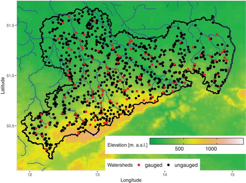
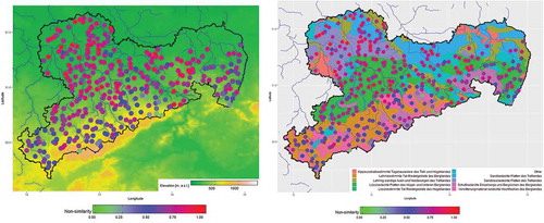
The database consists of 860 catchments in Saxony, eastern Germany, which mainly belong to the River Elbe Basin (Fig. 1). The catchments were selected by analysis of the river network, starting upstream with a minimum drainage area size of 10 km² and considering an increase in this drainage area by a tributary with a catchment of at least 10 km² at the point of confluence to specify the next point of the river network, where we estimated the catchment characteristics of the catchment in total. These catchments were separated into 11 classes according to their size to ensure that they can be considered as independent in their classes. To avoid bias, nested catchments were not included in these classes. In Saxony (area: 18 450 km²), the south is dominated by the Ore Mountains, with elevations of up to 1215 m a.s.l., whereas the northwestern parts are flatter, with elevations as low as 73 m a.s.l. The hydrological regions, as well as the land use, are very diverse in Saxony, with two large cities, Leipzig and Dresden, but also large areas of agriculture and forest. In Germany, Saxony has one of the densest and longest gauging networks, with most data available at the iDA (Interdisciplinary Data and Analyses) data centre.¹

Figure 1. Map of Saxony, Germany, with gauged and ungauged catchments. Points represent the centre of each catchment.

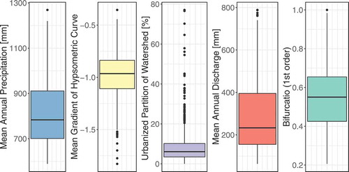
For the considered catchments, besides the area, 27 different characteristics are available, a full list of which is given in Table 1. The characteristics range from topographic aspects, such as river network density, slope of the hypsometric curve or bifurcation, to meteorological aspects, such as evaporation or mean annual precipitation. Selected characteristics are shown in Fig. 2 for all catchments, where the mean annual discharge was obtained with a water balance model, HAD_GW (Neumann 2009). Of these 865 catchments, 165 are already equipped with recording runoff gauges.

Table 1. Available characteristics of the catchments and explanations.

Parameter	Characteristic	Definition	Hydrological meaning
Length_riv_tot	Total length of river network, LK (km]	Sum of all length of rivers in a catchment	Impact on channel reservoir
Density	River network density, D = LK/AE (km^−1)	Relation between total length of river network and area of the catchment	Indicator for infiltration potential
TopoFactor	Topographical factor, TF = LK/√I (km)	Relation of total length of river network and the square root of mean elevation gradient, derived from raster data	Indicator for travel time
R95p_mean	Mean intensity of heavy rain events (mm/d)	Mean intensity of precipitation events that are larger than the 95% quantile of the period 1961–2010	Characteristic for extraordinary precipitation, impact on hydrograph shape
Hyps_Grad	First moment of hypsometric curve (-)	Mean gradient of hypsometric curve	Indicator for travel time and shape of hydrograph; characterizes dependence on height
Radian_0 = N	Aspect of mean flow direction (clockwise, starting north) (rad)	Radian measure for flow direction
Radian_0 = S	Aspect of mean flow direction (clockwise, starting south) (rad)
Relief	Relative relief, Δh/km2 (m^−1)	Mean difference of height per areal unit	Measure for cutting of catchment, the larger it is the more cut the aquifer
Circularity	Circularity relation, RC = AE/AC (-)	Relation between catchment area and the area of a circle with the same perimeter as the catchment	Impact on runoff concentration
Bifurcatio	Bifurcation	Geometric mean of river order	Coherence between number of reaches and their respective order; geological complexity of catchment
CorineField	Proportion of field (%)	Based on Corine land-use dataset version 13^3	Land use has impact on runoff generation
CorineForest	Proportion of forest (%)
CorineDevel	Proportion of development (%)
Mean_ann_prec	Mean annual precipitation height in 1961–2010 (mm)	Weighted mean by area per catchment0-based raster data (DWD 2012)	Characterizes climatic region
Max_daily_prec	Maximum daily precipitation height in 1901–2010 (mm)		Characterizes extreme precipitation
Freq_prec_larg	Frequency of daily precipitation height > 50 mm within 10 years in 1901–2010 (-)		Characterizes temporal distribution of extreme precipitation
CG1_mean	Storage constant, CG1 (d)	DIFGA^4 storage constant for short-term groundwater runoff (Schwarze et al. 1991)	Characterizes aquifer for short-term baseflow
CG2_mean	Storage constant, CG2 (d)	DIFGA storage constant for long-term groundwater runoff (Schwarze et al. 1991)	Characterizes aquifer for long-term baseflow
WSC_2 m	Water storage capacity of soil (mm)	Sum of available soil and air moisture up to thermocline or 2 m
meanHeight	Mean elevation (m a.s.l.)	Based on a 20-m raster	Indicator for local climate
meanGradient	Mean areal gradient (%)		Indicator for runoff components (fast and slow)
Length_main	Length of main river in catchment (km)
Riv_response	River network response	Number of stretches of rivers in consecutive unit ranges (5 km) beginning at the outlet (normalized by total number of stretches or river)	Characterizes the shape of the catchment with impact on peak and shape of hydrograph
Eff_evapo	Mean annual effective evaporation (mm)
Prec_wi_su	Sum of mean precipitation heights (corrected) of hydrological half year (mm)
Mean_ann_Q	Mean annual discharge (mm)
GW_recharge	Mean annual groundwater recharge (mm)

Figure 2. Boxplots of selected characteristics for all catchments.

The size of the catchments and their topographic and meteorological conditions vary greatly. Moreover, the dependencies between these characteristics also vary with size. This was the second reason for us to differentiate between classes of area, resulting in 11 different catchment classes (Table 2). For each of these catchments, explanatory characteristics were extracted from the list. To extend the available information, we also considered the option to enlarge the number of catchments by those that are 10% smaller or larger than the given bounds. This makes the bounds less restrictive.

Table 2. Classification of catchments according to area.

Name	Area included (km^2)	Number of catchments	Name	Area included (km^2)	Number of catchments
CC_10–30	10–30	376	CC_150–200	150–200	45
CC_30–50	30–50	151	CC_200–250	200–250	20
CC_50–75	50–75	83	CC_250–300	250–300	19
CC_75–100	75–100	55	CC_300–350	300–350	17
CC_100–125	100–125	48	CC_350–400	350–400	10
CC_125–150	125–150	36

It is not possible to consider all characteristics at the same time, since many of them are dependent on each other, e.g. the height is dependent on the area, or the land use is dependent on the altitude. Hence, for each class in Table 2, only characteristics with a Pearson correlation coefficient smaller than 0.6, compared to any other characteristic considered for that class, were used.

3 Methods

3.1 Maximum entropy

Entropy, as defined by Shannon (1948), measures the proportion of subjective choice in the selection of an event. More precisely, for a discrete random value X with possible values $X\mathrm{\prime }=\left\{x_1,\dots ,x_n\right\}$, the entropy, H, is defined as the expected value of the information content of value:

(1) $H=-\sum _{i=1}^n{p}_i\mathrm{l}\mathrm{o}{\mathrm{g}}_2\left(p_i\right)$(1)

where $p_i=P\left(X=x_i\right)$.

In the context of maximum entropy, the entropy is used to find the best approximation of an unknown distribution. That is, we want to find the approximation that fulfills any constraints of the unknown distribution that are known and, with regard to these constraints, has maximum entropy (Jaynes 1957). This means, we want to find the distribution that fulfills all necessary assumptions but nothing that is not needed (known) and would lead to unnecessary restriction. In our case, we are interested in the probability distribution p, whose approximation, $\hat{p}$, has entropy:

(2) $H\left(\hat{p}\right)=-\sum _{i=1}^n\hat{p}\left(x_i\right)\mathrm{l}\mathrm{n}\hat{p}\left(x_i\right)$(2)

To find this distribution, complex algorithms are needed. Here, we use the Maxent algorithm of Phillips et al. (2006), which is available as open-source software.² This approach defines the constraints on the distribution as real-value functions $f_1,\dots ,f_n$ of X, the so-called features, which in our case are catchment characteristics. The maximum entropy principle is then defined as the derivation of a probability distribution $\hat{p}$ of maximum entropy that fulfills the condition of equal expected value of each feature under the probability distribution $\hat{p}$, i.e.:

(3) $E_{\hat{p}}\left(f_j\right)=\sum _{i=1}^n\hat{p}\left(x_i\right)f_j\left(x_i\right)$(3)

as well as observed (derived by the empirical mean of a sample $x_1^{\prime },\dots ,x_k^{\prime }$ drawn from X under consideration of $\hat{p}$), i.e.:

(4) $E_{\hat{p}}\left(f_j\right)=\frac{1}{k}\sum _{i=1}^k{f}_j\left(x_i^{\prime }\right)\mathrm{f}\mathrm{o}\mathrm{r}\mathrm{a}\mathrm{l}\mathrm{l}j=1,\dots ,n$(4)

It can be shown that this is equal to applying a maximum likelihood procedure that searches iteratively for the solution by adjusting the weights λ of the Gibbs distribution:

(5) $q_{\lambda }\left(x\right)=\frac{\mathrm{e}\mathrm{x}\mathrm{p}\left(\lambda f\left(x\right)\right)}{Z_{\lambda }}$(5)

with f denoting the vector of all m features and $Z_{\lambda }$ being a normalizing constant, ensuring that $q_{\lambda }$ is a probability distribution. The starting point is the uniform distribution, where $\lambda =\left(0,\dots ,0\right)$. For more details, the reader is referred to Phillips et al. (2006).

3.2 Model evaluation

Following Phillips et al. (2006), the main criterion for model evaluation is the receiver operating characteristic (ROC), which is an unbiased threshold-independent measure often used in medical studies (Fielding and Bell 1997). The ROC technique evaluates the diagnostic ability of a receiver for a binary classification for varying thresholds (Deleo 1993). For every parameter set, the resulting relative frequency distributions are calculated. The corresponding plot, the ROC curve, is obtained by plotting the true positive rate (sensitivity) against the false positive rate. Simplified, also the cumulative distributions of both can be taken. If the ROC curve is close to the diagonal, this indicates a random process, since true and false positive classifications are equally probable. An ideal ROC curve increases almost vertically first, indicating high true classification compared to almost 0 false classification, and only increases horizontally if the value of 1 is nearly reached.

To obtain an index and make several models comparable, the area under curve (AUC) is often taken. Since a random model has equal sensitivity and false positive rate, its AUC is 0.5 and, hence, the lower limit, whereas the upper limit of the AUC is 1. Thus, a model with AUC close to 1 can be seen as preferable to a random model. More precisely, an AUC of 0.8 means that, in 80% of all cases, a random selection from the positive class will have a score larger than a random selection from the negative class (Fielding and Bell 1997).

3.3 Application to location of new gauges

While Phillips et al. (2006) used the Maxent algorithm to obtain probabilities for the occurrence of species in unobserved areas by using environmental characteristics, we applied it to obtain the probability of non-similarity of hydrological characteristics for a possible new gauge compared to existing gauges. In principle, the question is very similar, since in both cases environmental characteristics are used to obtain information on similarity of areas. For each catchment (observed or unobserved), all variables given in Table 1 are available and selected according to their dependence on each other for each class given in Table 2. The independent characteristics for each class are given in the Appendix (Table A1). Interestingly, the number of independent characteristics declines with increasing area of a catchment. The algorithm then calculates the probability of non-similarity for each catchment. High probability indicates that the allocation of a gauge at the outlet of this catchment would deliver additional information compared to all existing gauges. Moreover, by calculating the contribution of each considered characteristic on the entropy, we can evaluate which characteristic delivers the highest proportion of information. Of course, if dependent characteristics are used, this evaluation would not have much explanatory power.

Note that validation of the predictive power by using a test set of observed gauges is not possible in this case, since the observed gauges were not constructed under consideration of non-similarity.

3.4 Interactive application in an online GUI

To make the application easy to handle, especially for practitioners without programming skills, the algorithms were integrated in a Shiny application,⁵ “Saxontropy”, based on the programming language R (R Core Team 2018). To make a connection between R and the Maxent software possible, we used the R package dismo (Hijmans et al. 2017) together with RJava (Urbanek 2019). To enable topological and geographical classification of the catchments, several maps are available in the app: DEM (digital elevation model), Open Street Map and hydrological region, for which the R packages raster, rgdal, rgeos and sp were used. Moreover, a selection control was integrated, such that only predefined “geochores” or hydrological regions can be selected and included in the maximum entropy calculation. Thus, the informational content of new gauges for certain regions of interest can be evaluated directly. In addition, the catchment characteristics can be selected to consider only certain characteristics of interest. By default, the characteristics previously identified as independent for each catchment class (Table 2) are selected.

By selecting one catchment, the detailed probability of non-similarity of this catchment compared to catchments with measuring gauges is given, along with its identifying number. If the catchment is already gauged, the name of the gauge is also displayed and the probability of non-similarity can be interpreted as a measure for the similarity between all gauged catchments. To evaluate the impact of each selected characteristic, a contribution plot on the model is also displayed. Further details and the data of the model can be obtained by using the button “Maxent statistics”, which links directly to the model output given by the Maxent model implemented by Phillips et al. (2006).

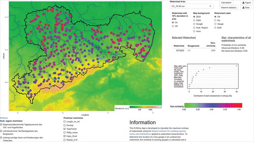
The Saxontropy app is freely available online⁶ (see Fig. 3 for an excerpt). Please note that, for the app, the original dataset has been scrambled to comply with data privacy laws. However, all relationships between the attributes have been preserved to demonstrate applicability.

Figure 3. Excerpt from the Online App “Saxontropy”.

4 Discussion

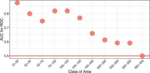
The MaxEnt model was applied to catchments of all area classes, in which gauged (runoff gauges) as well as ungauged catchments are available. The gauged catchments were used as basic information and their characteristics compared with those of the ungauged catchments. The MaxEnt algorithm then delivered a probability of non-similarity for each ungauged catchment in comparison with the group of gauged catchments within the same size class and, according to the selection of a sub-group, specified by predefined regions. Overall, the results concerning the model goodness of fit for the different area classes are very good. The AUC is much higher than it would be for a totally random model (UC = 0.5) for all classes up to 150 km² (Fig. 4) indicating a high explanatory power of the model. For larger catchments, it tends to 0.5, indicating that not much more information is included in the model than would have been in a random one. However, AUC greatly depends on the number of available catchments in a class. For catchments larger than 200 km², only fewer than 50 are available, and the AUC decreases rapidly. For up to about 75 catchments, the AUC is rather high and indicates good results. For comparison, in the following, two different area classes are evaluated in detail: “small catchments” of between 10 and 30 km² (the smallest class, with 374 catchments) and “large catchments” of between 150 and 200 km² (41 catchments).

Figure 4. Area under curve (AUC) for the ROC-curve for all classes of catchment area (including 10% deviation).

For the small catchments (10–30 km²), distinct patterns of non-similarity may be observed (Fig. 5). Whereas, for the southern and eastern catchments, a small probability (<0.5) is determined, the northwestern catchments deliver a high probability of non-similarity. In this area, the installation of new gauges would lead to new information and would be recommended. The catchments with the lowest probability (<0.25) are all located close to the Ore Mountains. Here, additional gauged catchments would not be sensible as most of the gauges in small catchments are located here. Dependence on hydrological region did not become visible in this case.

Figure 5. Probability of non-similarity of the small catchments to gauged catchments of the same size with underlying elevation model (left) and hydrological regions (right). A high probability of non-similarity close to 1 indicates probable additional information in this catchment.

This is in line with the results obtained when looking at the contribution of each variable on the model (Fig. 6). Here, it becomes obvious that mainly the topographical variables, in combination with climate, are responsible for the results. The highest contribution delivers the maximum daily precipitation, the effective evaporation and the topographical factor with about 60%. In addition, the shape of the catchment seems to be important.

Figure 6. (left) Contribution (in %) of each variable to the entropy model and (right) ROC plot of the fitted entropy model for small catchments. The straight line is the ROC curve for a totally random model.

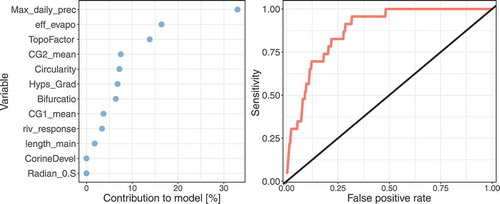
The ROC curve (Fig. 6) shows a large deviation from the random model and, hence, a good fit of the model for small catchments (AUC: 0.876). The results show that, for small catchments, the model delivers very good results and additional gauges should be built in the northern parts of the basin.

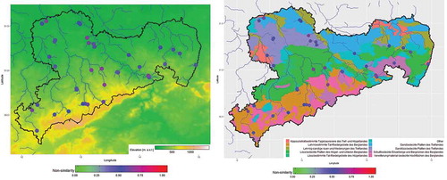
For the large catchments (150–200 km²), the results are not as good as for small catchments. Of course, only a small number of catchments is available in this class and none of these has a probability of non-similarity of more than 0.7 (Fig. 7). Catchments with the highest probability of non-similarity are located in the centre of the basin. If new gauges are necessary for this class, they should be built here. However, they probably will not deliver much additional information compared to those of smaller catchments.

Figure 7. (left) Probability of non-similarity of large catchments with underlying elevation model and (right) the hydrological regions. A high probability of non-similarity close to 1 indicates probable additional information in this catchment.

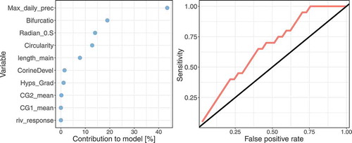
This result is also visible in the ROC curve (Fig. 8), which is much closer to a totally random model than for the small catchments. Hence, the MaxEnt model obtained for large catchments did not result in a good fit, with an AUC value of 0.659. However, similar characteristics to those for small catchments deliver the highest contribution to the model (Fig. 8). Again, the maximum daily precipitation is the most important characteristic and circularity and bifurcation, defining the shape of the catchment, contribute a great deal to the model.

Figure 8. (left) Contribution (in %) of each variable to the model and (right) ROC plot of the fitted model for large catchments. The straight line is the ROC curve for a totally random model.

What remains unclear is the relation between the non-similarity of catchments specified by their physical characteristics and the runoff conditions, which we are most interested in. In particular: does a high probability of non-similarity indicate different runoff characteristics that would justify the installation of a new gauge? Up to now, it is only assumed that the catchment characteristics considered here are directly related to the runoff and that a difference in these characteristics implies difference also in the runoff, but no proof is given. To evaluate this, hydrological signatures proposed by Sawicz et al. (2011) were applied. They can be used to classify catchments by clustering six signature characteristics based on daily discharge, precipitation and temperature: (1) the runoff ratio (ratio of discharge to precipitation over a large time scale), (2) the slope of the flow duration curve, (3) the baseflow index (ratio of baseflow to total runoff), (4) the streamflow elasticity (sensitivity of catchment reaction to precipitation on a larger time scale), (5) the snow day ratio (ratio of days with snowfall to days with precipitation) and (6) the rising limb density (ratio of the number of days with rising limbs to the number of total rising limbs). With these signatures, clustering of gauged catchments is possible, leading to clusters that significantly differ in their runoff behaviour. Analogous to Sawicz et al. (2011), here, the characteristics are clustered by the AutoClass algorithm developed by Stutz and Cheeseman (1995). This clustering is a probabilistic approach based on Bayesian mixture modelling, which has the advantage that the number of clusters does not have to be specified a priori, since the algorithm optimizes the number of classes with the Kullback-Leibler distance metric by using random starting clusters. This approach was applied to the small gauged catchments (10–30 km²) considered above. Considering that some of the gauges were installed for control purposes, e.g. downstream of reservoirs, 17 gauges remained for this analysis. The clustering resulted in three clusters. Note that, due to the Bayesian clustering approach chosen, each data point does not belong to a unique cluster; instead, the probabilities of belonging to one cluster are given. In particular, at the edges of each cluster, probabilities are similar for two clusters and, hence, also a different clustering could be possible. However, we decided to choose the cluster with the highest probability for each data point. Using this clustering, in a next step one cluster is selected. Each catchment belonging to this cluster is marked as ungauged. Then, the maximum entropy approach based on the catchment characteristics presented above (no discharge was included) is applied to all three clusters. Two are labelled as gauged but the selected one is labelled ungauged. Thus, a probability of non-similarity for the left-out (ungauged) cluster is obtained compared to the two remaining clusters. If runoff behaviour were connected to high values of non-similarity, the obtained probabilities of non-similarity should be higher for the left-out cluster, since the clusters are obtained by signatures related to discharge. Figure 9 shows the three resulting cases of one left-out cluster. It can be seen that the probability of non-similarity of the maximum entropy approach of the left-out cluster is significantly larger than for the remaining clusters. This leads to the conclusion that the results of the maximum entropy approach deliver results that are closely connected to the runoff behaviour of a catchment, although discharge was not used as a characteristic in the MaxEnt approach. More precisely, a high value of non-similarity obtained by the maximum entropy of catchment characteristics indicates a difference in the clusters that are defined by runoff signatures and vice versa.

Figure 9. Comparison of probabilities of non-similarity of the maximum entropy approach when leaving one cluster out. Clusters are obtained by hydrological signatures.

While this paper tries to reduce the uncertainty of the hydrometric network design by building gauges in catchments where the transinformation is low, there also might be uncertainties in data and catchment division beforehand. Here, the entropy is mainly based on measured and consequently interpolated data, as well as some modelled data. Single outliers can likely be detected when analyzing the catchment with the lowest and highest probability of non-similarity (and therefore the best/worst future gauging solution) in-depth, e.g. looking at the contribution of input data to the model. Also, uncertainty can be introduced by the division of catchments (see Section 2). A different classification system, e.g. by aquifer or assignment to counties, would result in different catchments and therefore a different maximum entropy. Most importantly, a well-documented database and communication with local (water) authorities are crucial for obtaining a high-quality database as input for the entropy model, as well as many other applications.

5 Summary and conclusion

The maximum entropy approach was applied to catchment characteristics of gauged and ungauged catchments to evaluate which of the ungauged catchments would deliver the highest amount of new hydrological information if it became gauged. By using a simple Shiny application, this tool supports practitioners to improve the decision process on integrating new gauges in hydrometric networks. Model evaluation tools like the ROC or AUC can be used to investigate the goodness of fit of the model, while the contribution of each catchment characteristic on the model contains information on the type of new information that would be obtained by supplementary gauges. To omit dependencies of the characteristics, these were pre-selected and the catchments were divided into different classes according to their size.

The results of the entropy model show that, especially for small catchments up to 150 km², the MaxEnt model delivers a good fit, with high AUC values. For larger catchments, the fit is not as good, mainly because of the reduced number of catchments available in this class. Nevertheless, for all classes, the high importance of the maximum daily precipitation in the catchment, as well as the shape of the catchment, was observed when the information should be maximized. This is similar to the early approaches of network optimization by Karasev (1968), who based his approach also on geographical attributes. Moreover, many regression approaches also focus on these characteristics. Characteristics such as effective evaporation only contribute to the model for small catchments. This coincides with the results of Oudin et al. (2005a, 2005b), who found that evaporation did not improve hydrological models much for large catchments. The hydrological region and land use do not play a crucial role for the obtained new information. In a second step, the results were linked to hydrological signatures. Thus, it was concluded that a relation between the probabilities of non-similarity obtained by characteristics that do not include discharge and the runoff behaviour of a catchment should be quantified. By a leave-one-out approach, it was shown that, indeed, the clusters obtained by the hydrological signatures are correlated with the resulting probability of non-similarity. Hence, it can be concluded that the runoff behaviour of an ungauged catchment is different from that of all gauged catchments if the probability of non-similarity obtained with characteristics used here is high.

It becomes clear that the manual allocation of additional gauges is very difficult when the aim is to obtain as much new information as possible. Regional physical characteristics do not play a crucial role, whereas the shape of the catchment and meteorological characteristics do. In addition, the relevance of these parameters varies with catchment size. The Saxontropy tool can be used to help in the allocation of additional gauges in river basins and also delivers an assessment of the opportunities to get additional information about the runoff behaviour of an ungauged catchment compared to all gauged catchments. For most authorities, the installation of all possible gauges is not feasible due to financial constraints. This tool can be used as a selection criterion for new gauges and the benefit of a newly installed gauge can be maximized; and this can be done for different catchment sizes. The additional information is important for practitioners as well as scientists. For practitioners, it delivers an objective criterion for the extension of the existing gauging network, while for scientists, the extension of the dataset under the aspect of information extension is beneficial for, e.g. flood statistics and regionalization or deterministic modelling, where information extension plays a crucial role. In the context of big data and machine learning, in particular, high information content in large datasets is of utmost importance.

Acknowledgements

The authors would like to thank the Saxon State Office for Environment, Agriculture and Geology in Germany for providing the extensive database for this study and Kariem A. Ghazal as well as an anonymous reviewer for their helpful comments that helped to improve the manuscript.

Disclosure statement

No potential conflict of interest was reported by the authors.

Additional information

Funding

The financial support of the German Research Foundation (Deutsche Forschungsgemeinschaft, DFG) in terms of the research unit SPATE (FOR 2416) for Philipp Bühler, Svenja Fischer and Andreas Schumann is gratefully acknowledged.

Notes

¹ https://www.umwelt.sachsen.de/umwelt/infosysteme/ida

² http://biodiversityinformatics.amnh.org/open_source/maxent/.

³ CORINE is a satellite-based inventory of land cover in 44 classes. The version used here is available at http://www.eea.europa.eu/data-and-maps/data#c12=corine+land+cover+version+13.

⁴ DIFGA is an inverse approach that assesses runoff components based on flow recession curves. More details are given in Schwarze et al. (1991).

⁵ https://shiny.rstudio.com/.

⁶ www.github.com/PhilippBuehler/Saxontropy.

Appendix.

Table A1. Independent (×) characteristics used for the maximum entropy approach for each catchment class.

Characteristic	CC_10-30	CC_30-50	CC_50-75	CC_75-100	CC_100-125	CC_125-150	CC_150-200	CC_200-250	CC_250-300	CC_300-350	CC_350-400
TopoFactor	×	×				×
Hyps_Grad	×	×	×	×	×	×	×	×	×	×
Radian_0 = S	×	×	×	×	×	×	×		×	×
Circularity	×	×	×	×	×	×	×			×
Bifurcatio	×	×	×	×	×	×	×	×	×	×	×
CorineDevel	×	×	×	×	×	×	×	×	×	×
Max_Daily_prec	×	×	×	×	×	×	×		×	×	×
CG1_mean	×	×		×	×		×	×	×	×	×
CG2_mean	×	×	×	×	×	×	×	×
Length_main	×	×	×	×	×	×	×	×		×
Riv_response	×	×	×	×	×	×	×	×
Eff_evapo	×

References

- Alfonso, L., Lobbrecht, A., and Price, R., 2010. Information theory–based approach for location of monitoring water level gauges in polders. Water Resources Research, 46, W12553. doi:10.1029/2009WR008101
- Alizadeh, Z., Yazdi, J., and Moridi, A., 2018. Development of an entropy method for groundwater quality monitoring network design. Environmental Processes, 5, 769–788. doi:10.1007/s40710-018-0335-2
- Banik, B.K., et al., 2017. Evaluation of different formulations to optimally locate pollution sensors in sewer systems. ASCE Journal of Water Resources Planning, 143 (7).
- Blöschl, G. and Sivapalan, M., 1995. Scale issues in hydrological modelling: a review. Hydrological Processes, 9, 251–290. doi:10.1002/hyp.3360090305
- Chacon-Hurtado, J.C., Alfonso, L., and Solomatine, D.P., 2017. Rainfall and streamflow sensor network design: a review of applications, classification, and a proposed framework. Hydrology and Earth System Sciences, 21, 3071–3091. doi:10.5194/hess-21-3071-2017
- Deleo, J.M., 1993. Receiver operating characteristic laboratory (ROCLAB): software for developing decision strategies that account for uncertainty. In: Proceedings of the Second International Symposium on Uncertainty Modelling and Analysis. College Park, MD: IEEE Computer Society Press, 318–325.
- Fielding, A.H. and Bell, J.F., 1997. A review of methods for the assessment of prediction errors in conservation presence/absence models. Environmental Conservation, 24 (1), 38–49. doi:10.1017/S0376892997000088
- Fuentes, M., Chaudhuri, A., and Holland, D.H., 2007. Bayesian entropy for spatial sampling design of environmental data. Environmental Ecology and Statistics, 14, 323–340. doi:10.1007/s10651-007-0017-0
- Hijmans, R.J., et al., 2017. dismo: species distribution modeling. R package version 1.1-4. Available from: https://CRAN.R-project.org/package=dismo [accessed 12 January 2020].
- Jaynes, E.T., 1957. Information theory and statistical mechanics, I. Physical Reviews, 106, 620–630. doi:10.1103/PhysRev.106.620
- Joo, H., et al., 2019. Optimal stream gauge network design using entropy theory and importance of stream gauge stations. Entropy, 21, 991. doi:10.3390/e21100991
- Karasev, I.F., 1968. On the principles of hydrological network design and prospective development. Trans. State Hydrol. Inst. Trudy GGI, 164, 3–36. (In Russian; English version in Soviet Hydrology, 6, 560–588, 1968).
- Keum, J., et al., 2018. Application of SNODAS and hydrologic models to enhance entropy-based snow monitoring network design. Journal of Hydrology, 561, 688–701. doi:10.1016/j.jhydrol.2018.04.037
- Keum, J., et al., 2017. Entropy applications to water monitoring network design: a review. Entropy, 19 (11), 613. doi:10.3390/e19110613
- Krstanovic, P.F. and Singh, V.P., 1992. Evaluation of rainfall networks using entropy: I. Theoretical development. Water Resources Management, 6, 279–293. doi:10.1007/BF00872281
- Mishra, A.K. and Coulibaly, P., 2009. Developments in hydrometric network design. A review. Reviews of Geophysics, 47 (2), 1491. doi:10.1029/2007RG000243
- Neumann, J., 2009. Flächendifferenzierte Grundwasserneubildung von Deutschland. Stuttgart, Germany: Schweizerbart.
- Oudin, L., et al., 2005a. Which potential evapotranspiration input for a lumped rainfall-runoff model? Part 2 – towards a simple and efficient potential evapotranspiration model for rainfall-runoff modelling. Journal of Hydrology, 303, 290–306. doi:10.1016/j.jhydrol.2004.08.026
- Oudin, L., Michel, C., and Anctil, F., 2005b. Which potential evapotranspiration input for a lumped rainfall-runoff model? Part 1 – can rainfall-runoff models effectively handle detailed potential evapotranspiration inputs? Journal of Hydrology, 303, 275–289. doi:10.1016/j.jhydrol.2004.08.025
- Phillips, S.J., Anderson, R.P., and Schapire, R.E., 2006. Maximum entropy modeling of species geographic distributions. Ecological Modelling, 190, 231–259. doi:10.1016/j.ecolmodel.2005.03.026
- Pyrce, R.S., 2004. Review and analysis of stream gauge networks for the Ontario stream gauge rehabilitation project. Peterborough, Ontario: Trent University, Watershed Science Centre. WSC Report No. 01-2004. Prepared for the Ontario Ministry of Natural Resources and Forestry. https://www.trentu.ca/iws/documents/Network_Design_Mar04.pdf.
- R Core Team, 2018. R: A language and environment for statistical computing. Vienna, Austria, R Foundation for Statistical Computing. Available from: https://www.R-project.org/ [accessed 12 January 2020].
- Sawicz, K., et al., 2011. Catchment classification: empirical analysis of hydrologic similarity based on catchment function in the eastern USA. Hydrology and Earth System Sciences, 15, 2895–2911. doi:10.5194/hess-15-2895-2011
- Schwarze, R., et al., 1991. Rechnergestützte Analyse von Abflusskomponenten und Verweilzeiten in kleinen Mittelgebirgseinzugsgebieten [Computer assisted analysis of runoff components and transit times in small catchments, in German]. Acta Hydrophysica, 35 (2), 143–184, Berlin.
- Shannon, C.E., 1948. A mathematical theory of information. The Bell System Technical Journal, 27 (3), 379–423. doi:10.1002/j.1538-7305.1948.tb01338.x
- Singh, V.P., 1989. Hydrologic modelling using entropy. Journal of the Institute of Engineering, Civil Engineering Division, 70, 55–60.
- Singh, V.P. and Fiorentino, M., 1992. A historical perspective of entropy applications in water resources’. In: V.P. Singh and M. Fiorentino, eds. Entropy and energy dissipation in water resources. Dordrecht, The Netherlands: Kluwer, 155–173.
- Stutz, J. and Cheeseman, P., 1995. AutoClass – a Bayesian approach to classification. In: J. Skilling and S. Sibisi, eds.. Maximum entropy and bayesian methods, Cambridge 1994. Dordrecht, The Netherlands: Kluwer, 117–126.
- Urbanek, S., 2019. rJava: low-level R to java interface. R package version 0.9-11. Available from: https://CRAN.R-project.org/package=rJava [accessed 12 January 2020].
- Wang, W., et al., 2018. Optimization of rainfall networks using information entropy and temporal variability analysis. Journal of Hydrology, 559, 136–155. doi:10.1016/j.jhydrol.2018.02.010
- WMO, 2008. Guide to hydrometeorological practices. 6st ed. Geneva, Switzerland: World Meteorological Organization, WMO No.168, TP 82, ISBN 978-92-63-10168–6.
- Yang, Y. and Burn, D.H., 1994. An entropy approach to data collection network design. Journal of Hydrology, 157 (1–4), 307–324. doi:10.1016/0022-1694(94)90111-2
- Yoo, C., Ku, H., and Kim, K., 2011. Use of a distance measure for the comparison of unit hydrographs. Application to the stream gauge network optimization. Journal of Hydrologic Engineering, 16 (11), 880–890. doi:10.1061/(ASCE)HE.1943-5584.0000393