Re-initiating depth-discharge monitoring in small-sized ungauged watersheds by combining remote sensing and hydrological modelling: a case study in Madagascar

ABSTRACT

This work presents a practical approach to reconstructing past and present discharge and water depth time series for operational monitoring of small-sized ungauged watersheds using remotely sensed and freely accessible datasets in conjunction with hydrological models. The methodology was applied to the Tsiribihina watershed in Madagascar. Mostly, satellite data are used, such as water levels from satellite altimetry missions and rainfall from the African Rainfall Climatology 2 product. In contrast, the Modelo de Grandes Bacias is calibrated using historical discharge measurements to simulate distributed discharge in the basin. Rating curves are computed by crossing the altimetry information of water height with the simulated discharge outputs. These rating curves enable the conversion of water levels, discharge and depth interchangeably. Present-day discharge and depth can thus be estimated in near real time with any update of satellite rainfall data and/or water level gained by altimetry missions currently flying in operational mode.

KEYWORDS:

• water level
• depth
• rainfall–discharge model
• altimetry
• Tsiribihina
• Madagascar

Editor A. Castellarin Associate editor A. Domeneghetti

1 Introduction

In evaluating available water resources, building water-related infrastructures such as dams and forecasting extreme hydrological events such as droughts or floods, knowledge of river discharge and its long-term variability is necessary (Lebecherel et al. 2015). Water infrastructures and water-management systems are designed based on historical observations of hydrological data (Cosgrove and Loucks 2015). Therefore, hydrological data such as depth and discharge are important.

Water level, depth and discharge are traditionally measured at gauging stations emplaced at a few key locations in the watersheds. However, the number of such gauging stations has decreased worldwide over recent decades (Pavelsky et al. 2014, GRDC 2016) or is under risk of future decline (World Water Assessment Programme 2009). Water resources cannot be managed adequately unless hydrological data exist (Stewart 2015). Hence, past temporal gaps and the lack of up-to-date information in time series compromise the validity of information. The absence of such information for use in assessing the water resources and the dynamics of flow may prevent wise water management-related decisions.

Methodologies have been proposed in the literature to solve for the gaps in or the lack of hydrometric data (Post and Jakeman 1999, Allasia et al. 2006, Leon et al. 2006, Young 2006, Bárdossy 2007, Bodian 2012, Boughton and Chiew 2007, Castiglioni et al. 2010, Mdee 2015, Revilla-Romero et al. 2015, Van Emmerik et al. 2015, Paris et al. 2016, among others). However, these methods have been mostly applied on large river basins, such as the Amazon. This work aims to adapt and evaluate existing methodologies in reconstructing past and present depth-discharge time series for operational monitoring of relatively small rivers, using mostly remotely sensed data combined with hydrological modelling.

Remote sensing techniques provide the capacity to gather information remotely and routinely about the Earth’s surface with global coverage. It demonstrated excellent capability to monitor surface waters (Cazenave et al. 2016). It has been used for flood monitoring (Irimescu et al. 2009, Klemas 2014, Schumann 2015, Twele et al. 2016, among others), for monitoring water quality (Abdelmalik 2016, Gholizadeh and Melesse 2017, Hansen et al. 2017, Rostom et al. 2017, among others) and to monitor water levels in lakes, large rivers and floodplains using satellite radar altimeters (Birkett 1998, Maheu et al. 2003, Kouraev et al. 2004, Frappart et al. 2006, Kosuth et al. 2006, Papa et al. 2010, Roux et al. 2010, Silva et al. 2010, Asadzadeh Jarihani et al. 2013, Maillard et al. 2015, Coss et al. 2020, among others). Nearly three decades of water-level time series can be constructed for inland waters from a series of satellite radar altimetry missions, such as Topography Experiment or TOPEX/POSEIDON, JASON-1, JASON-2, JASON-3, European Remote-Sensing Satellite or ERS-2, ENVIronment SATellite or ENVISAT and Satellite with ARgos and ALtiKa SARAL. Water level can be used to derive river discharge (Bjerklie et al. 2003, Coe and Birkett 2004, Kouraev et al. 2004, Leon et al. 2006, Zakharova et al. 2006, Getirana et al. 2009, Birkinshaw et al. 2010, Papa et al. 2010, Getirana and Peters-Lidard 2013, Tarpanelli et al. 2013, Tourian et al. 2013, 2017, Paris 2015, Paris et al. 2016, Sichangi et al. 2016) and river altitude profiles (Leon et al. 2006, Getirana et al. 2009, Garambois et al. 2017).

In practice, depth is obtained from field measurements, including river cross-section bottom elevation. Remote sensing-based methods of determining depth include airborne or satellite-mounted light detection and ranging (LiDAR) (Pan et al. 2015, Bizzi et al. 2015, among others), but these methods are expensive and appear to be inappropriate for long-term studies. Multispectral and hyperspectral images offer interesting alternatives. These methods exploit the difference in sunlight attenuation at different wavelengths to deduce depth-related information and to produce bathymetry maps (Lyzenga et al. 2006, Legleiter et al. 2009, Morel and Favoretto 2017, among others). Other methods combine light information with flow hydraulic considerations (Fonstad and Marcus 2005, Legleiter 2015). However, when long depth-time series are needed, these methods become difficult to implement, particularly at the daily time step, as image time series are manipulated. It is also known that depth retrieval from images is limited by water clarity or turbidity conditions.

Rainfall discharge models allow simulation of river discharge, ranging from annual to sub-hourly time steps, using information on hydro-meteorological and environmental conditions. Such models can also be used to estimate the dynamics of the water cycle in areas of interest that are far from gauges (Bárdossy 2007). They have been used to fill data gaps and (re)construct longer records of still functioning or unmaintained gauges (Bodian 2012, Revilla-Romero et al. 2015). Models have also been used to predict discharge in ungauged basins (Post and Jakeman 1999, Allasia et al. 2006, Young 2006, Bárdossy 2007, Boughton and Chiew 2007, Castiglioni et al. 2010, Van Emmerik et al. 2015, Mdee 2015, Revilla-Romero et al. 2015, among others).

In this work, incomplete in situ hydrological data, satellite-based rainfall and altimetric data and hydrological models are used to reconstruct and update discharge and depth time series in a small-sized ungauged watershed, the Tsiribihina River, in Madagascar. We make use of the Modelo de Grandes Bacias (MGB) distributed rainfall–discharge model (Collischonn et al. 2007a, Paiva et al. 2011) to predict discharge time series distributed throughout the basin. Generally, geomorphological relations are used in hydrological models for the joint estimation of discharge and depth. For example, Andreadis et al. (2013) combined the geomorphological relations developed by Moody and Troutman (2002) with discharge taken from HydroSHEDS (Lehner and Grill 2013). These relations are usually spatial averages, such as at the regional scale, at the basin scale or for a given river channel reach, but are not specific to a river cross section. Consequently, they cannot be used to relate water level and discharge if both quantities are not derived by the model itself. Since we aim to use model-independent water levels obtained from satellite altimeters at crossings between the orbit ground tracks and the rivers, we must derive site-specific relations between the discharge simulated by the model and the aforementioned water levels. Finally, we force the mathematical expression of the rating curves to follow the physically based Manning’s equation to enable conversion among water level, discharge and depth.

2 Study area

The Tsiribihina River is the third largest river in Madagascar in terms of river basin extent (49 800 km²) (Chaperon et al. 1993). This river basin is chosen as the study case because of its economic importance for Madagascar, although it is no longer monitored. Its significant surface water and groundwater resources, and thus irrigation potential, predispose this basin to agriculture (Baudin 1982, Office Nationale pour l’Environnement 2017). Cultivable lands are used for food, cash and industrial crops (World Wide Fund 2011). Significant hydro-agricultural developments have been implemented (Fonds Africain de Développement 1994, Fonds International de Développement Agricole 2013, Présidence de la République de Madagascar 2017). However, water mismanagement has been noted to be the main cause of production decrease (Food and Agriculture Organization of the United Nations, World Food Program 2013). Unfortunately, water monitoring infrastructures have not been maintained properly (Lebigre 1988).

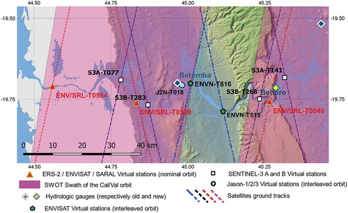
As illustrated in Fig. 1, the river basin of the Tsiribihina occupies the middle of the western side of Madagascar. The basin is bordered to the north by the basins of the Betsiboka and Manambolo rivers. On the south, it is limited by the basins of the Morondava and Matsiatra rivers. Ankaratra Mountain borders the basin on the east. The relief of the basin is globally descending from the centre of Madagascar Island towards the west coast. The highest altitude is that of Ankaratra Mountain, which reaches 2 643 m. The mean elevation is 919 m (green in Fig. 1). The Tsiribihina River is formed by its tributaries Sakeny, flowing from south to north; Manandaza, flowing from north to south; Mahajilo, in the northeast, and Mania, in the southeast, both originating from high altitudes and flowing westward through the central tableland. The last two rivers are the principal tributaries of the Tsiribihina River (Chaperon et al. 1993). The Tsiribihina River runs through the calcareous plateau of Bemaraha and continues its course to the ocean through a low-declivity area with several lakes and floodplains.

Figure 1. Study area with historical rain gauges and hydrological gauges. The background colour code relies on the elevation (in $\mathrm{m}$) in the Tsiribihina River basin

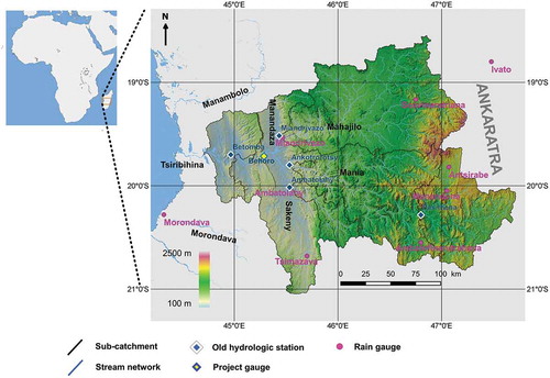
Figure 2. Mean annual rainfall (in $\mathrm{m}\mathrm{m}$) between 2000 and 2015 in the Tsiribihina River basin, computed from African Rainfall Climatology 2.0 or ARC2 data

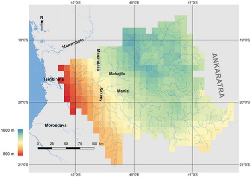
Savanna is the dominant vegetation, but sparse and dense tropophyl forests exist on the western side of the basin (Baudin 1982). The river basin lies in the sub-humid climate region with an annual rainfall of approximately 1 500 mm and a mean annual temperature exceeding 25°C (Chaperon et al. 1993). The rainy season starts in November and ends in March. The spatial distribution of inter-annual rainfall data in the river basin is presented in Fig. 2.

3 Methods

3.1 Discharge modelling

The MGB is a large-scale distributed and process-based hydrological model (Collischonn et al. 2007a, Getirana et al. 2009, Paiva et al. 2011) primarily designed for large basins and to address data scarcity (Getirana et al. 2009). The output of the model is the daily discharge series distributed on elementary catchments. To predict discharge distributed throughout a basin, the MGB requires basic records of hydro-meteorological variables, watershed elevation, land cover and soil maps to represent the physical and hydrological processes. The watershed is discretized into elementary catchments that are interconnected with channels following the method described by Maidment (2002) and using Geographic Information System or GIS-based algorithms (Paiva et al. 2011).

The model uses the concept of a hydrological response unit (HRU). An HRU characterizes areas with similar hydrological behaviour (Kouwen et al. 1993, Beven 2001). Categories of HRUs are built from a combination of types of land cover and types of soil. Each elementary catchment is composed of a parsimonious number of HRUs. The soil water balance is computed independently for each HRU by considering soil as a single layer and using components describing canopy interception, evapotranspiration, infiltration, surface runoff, subsurface flow, base flow and soil water storage (Collischonn et al. 2007b).

Canopy interception is represented by a reservoir whose maximum storage is a function of the vegetation leaf area index (LAI). The energy budget is computed using basic surface meteorological variables, and the computation of evapotranspiration is based on the Penman-Monteith approach (Collischonn et al. 2007a). Infiltration and surface runoff are estimated using the concept of variable contributing area of the ARNO model (Todini 1996). Subsurface flow is computed using an equation similar to the Brooks and Corey unsaturated hydraulic conductivity (Rawls et al. 1993). Percolation to the groundwater is obtained from a simple linear relation between soil water storage and maximum soil water storage (Paiva et al. 2011).

Three linear reservoirs collect the surface flow, the subsurface flow and the base flow generated by every HRU of an elementary catchment and routed further to the stream network (Collischonn et al. 2007a, Paiva et al. 2011). Then, the river flow is routed through the river network using the Muskingum-Cunge method (Cunge 1969).

The river basin border, sub-catchment upstream hydrological gauges, elementary catchments, and river network are delineated using GIS software. Geomorphological parameters such as width, length and bed slope of the river reach of each elementary catchment are also extracted from the elevation map. These parameters are used in the Muskingum-Cunge river flow routing (Getirana et al. 2009).

The MGB is run using daily meteorological variables (i.e. rainfall, temperature, humidity, wind speed, pressure and solar radiation, as described in Appendix A) and corresponding climatology. These variables are interpolated to the centre of each elementary catchment from stations or cell centres of satellite-based data using the classical inverse distance weighting (IDW) method (Chen and Liu 2012). Note that missing values for the variables other than rainfall are replaced by climatologies.

The MGB must be tuned to the specificity of each basin, and model parameters must be calibrated. These parameters are the maximum soil water storage, the spatial distribution of saturated soil within the elementary catchment, the hydraulic conductivity of the unsaturated zone of the soil layer, the percolation rate to the groundwater and the response times of the surface, interflow and base flow reservoirs. The first four parameters are relative to runoff generation at the HRU level, while the last three are relative to routing of flow inside the elementary catchments. Manual and automatic calibrations are performed successively by visual comparison of observed and simulated discharge hydrographs and/or by assessing performance indices, which will be described later. First, the response time of the base flow is estimated from the recession of an observed hydrograph. Then, the parameters relative to runoff generation are calibrated by checking the overall runoff volume error, the low-flow part of hydrographs, and the amplitude and timing of peaks. After that, the remaining parameters related to flow routing are calibrated. Automatic calibration is finally run to fine-tune all the values. This step is performed by multi-objective optimization of performance indices (Yapo et al. 1998). These performance indices are the Nash-Sutcliffe model efficiency coefficient (NS, Equation 1(1) $\mathrm{N}\mathrm{S}=1-\frac{\sum {\left(Q_{\mathrm{o}\mathrm{b}\mathrm{s}}-Q_{\mathrm{c}\mathrm{a}\mathrm{l}}\right)}^2}{{\sum }^{\hspace{0.17em}}{\left(Q_{\mathrm{o}\mathrm{b}\mathrm{s}}-\overline{Q_{\mathrm{o}\mathrm{b}\mathrm{s}}}\right)}^2}$(1) ), the Nash-Sutcliffe coefficient calculated on logarithms of the discharge values (NS-log, Equation 2)(2) $\text{{rm{N}}{{rm{S}}\_{{rm{log}}}} = 1 - {{{{mathop sum nolimits^ }^{}}{{left({{rm{log}}{Q\_{{rm{obs}}}} - {rm{log}}{Q\_{{rm{cal}}}}} right)}^2}} over {{{mathop sum nolimits^ }^{}}{{left({{rm{log}}{Q\_{{rm{obs}}}} - {rm{log}}overline {{Q\_{{rm{obs}}}}} } right)}^2}}}{rm{ }}}$(2) and the relative streamflow volume error (ΔV, Equation 3(3) $\mathrm{\Delta }V=\frac{\sum Q_{\mathrm{c}\mathrm{a}\mathrm{l}}-\sum Q_{\mathrm{o}\mathrm{b}\mathrm{s}}\hspace{0.17em}}{\sum Q_{\mathrm{o}\mathrm{b}\mathrm{s}}\hspace{0.17em}}\times 100$(3) ) (Collischonn et al. 2007a). The streamflow volume error is also a measure of the bias between observed and simulated discharge (Moriasi et al. 2007). The NS and NS-log can take values from −∞ to 1 where the optimal value is 1. The optimal value of ΔV is 0. The NS is slightly sensitive to systematic low-flow discrepancies (Krause et al. 2005). Therefore, the NS is regarded as a criterion of the efficiency of high-flow simulation (Oudin et al. 2006, Pushpalatha et al. 2012). The NS-log gives more emphasis to low-flow errors (Krause et al. 2005, Pushpalatha et al. 2012) and is used to evaluate modelling performance of low-flow conditions:

(1) $\mathrm{N}\mathrm{S}=1-\frac{\sum {\left(Q_{\mathrm{o}\mathrm{b}\mathrm{s}}-Q_{\mathrm{c}\mathrm{a}\mathrm{l}}\right)}^2}{{\sum }^{\hspace{0.17em}}{\left(Q_{\mathrm{o}\mathrm{b}\mathrm{s}}-\overline{Q_{\mathrm{o}\mathrm{b}\mathrm{s}}}\right)}^2}$(1)

(2) $\text{{rm{N}}{{rm{S}}\_{{rm{log}}}} = 1 - {{{{mathop sum nolimits^ }^{}}{{left({{rm{log}}{Q\_{{rm{obs}}}} - {rm{log}}{Q\_{{rm{cal}}}}} right)}^2}} over {{{mathop sum nolimits^ }^{}}{{left({{rm{log}}{Q\_{{rm{obs}}}} - {rm{log}}overline {{Q\_{{rm{obs}}}}} } right)}^2}}}{rm{ }}}$(2)

(3) $\mathrm{\Delta }V=\frac{\sum Q_{\mathrm{c}\mathrm{a}\mathrm{l}}-\sum Q_{\mathrm{o}\mathrm{b}\mathrm{s}}\hspace{0.17em}}{\sum Q_{\mathrm{o}\mathrm{b}\mathrm{s}}\hspace{0.17em}}\times 100$(3)

$\hspace{0.17em}{Q}_{\mathrm{c}\mathrm{a}\mathrm{l}},Q_{\mathrm{o}\mathrm{b}\mathrm{s}}\mathrm{a}\mathrm{n}\mathrm{d}\overline{Q_{\mathrm{o}\mathrm{b}\mathrm{s}}}$ denote the calculated discharge, the observed discharge and the mean observed discharge, respectively.

The quality of the calibrated parameters, and therefore of the simulation, is evaluated in a validation step where observed discharge is compared to simulated discharge. Hence, hydro-meteorological variables are split into two temporally non-overlapping blocks: the first one for calibration and the second one for validation of the parameters.

Initial values of the parameters are taken from Allasia et al. (2006), Collischonn et al. (2007a) and Paiva et al. (2011). The model can be run with at most 12 categories of HRUs. The dominant (most abundant) HRUs are calibrated first, and default values are kept for the remaining HRUs.

3.2 Depth estimation

3.2.1 Water levels from satellite altimetry

Crossings of the ground tracks of the satellite orbit with rivers are called virtual stations (VS) (Silva et al. 2010). One can extract an estimate of the water level at these VSs every time the satellite passes at the zenith of these VSs. The frequency of the sampling is given by the repeat cycle of the orbit, e.g. 35 days for ENVISAT and SARAL missions. The altimetry data are processed following the methodology developed by Frappart et al. (2006) and Silva et al. (2010). This methodology is based on the radar ranges derived by the ICE-1 retracking algorithm (Wingham et al. 1986). Frappart et al. (2006) and Silva et al. (2010) showed that the ICE-1 algorithm gives the best and most robust results over rivers. The water level of the water body is obtained by:

(4) $H=\mathrm{A}\mathrm{l}\mathrm{t}-R+\mathrm{\Delta }{R}_{\mathrm{p}\mathrm{r}\mathrm{o}\mathrm{p}\mathrm{a}\mathrm{g}}+\mathrm{\Delta }{R}_{\mathrm{g}\mathrm{e}\mathrm{o}\mathrm{p}\mathrm{h}\mathrm{y}}+N$(4)

In Equation (4)(4) $H=\mathrm{A}\mathrm{l}\mathrm{t}-R+\mathrm{\Delta }{R}_{\mathrm{p}\mathrm{r}\mathrm{o}\mathrm{p}\mathrm{a}\mathrm{g}}+\mathrm{\Delta }{R}_{\mathrm{g}\mathrm{e}\mathrm{o}\mathrm{p}\mathrm{h}\mathrm{y}}+N$(4) , Alt is the height of the satellite orbit above a reference ellipsoid and R is the range measured from the travel time of the radar pulse using a retracking algorithm. The $\mathrm{\Delta }R$ terms are corrections to the range, taking into account the fact that the radar pulse is delayed during its propagation into non-vacuum media, namely the ionosphere and the troposphere, and that the surface of the Earth is permanently deformed by geophysical phenomena such as tides and departs from the reference ellipsoid. Following Fernandes et al. (2014), the Global Ionosphere Map (GIM) and the European Centre for Medium-Range Weather Forecasts or ECMWF-based corrections are used for the ionospheric, dry and wet tropospheric corrections. The last term N in Equation (4)(4) $H=\mathrm{A}\mathrm{l}\mathrm{t}-R+\mathrm{\Delta }{R}_{\mathrm{p}\mathrm{r}\mathrm{o}\mathrm{p}\mathrm{a}\mathrm{g}}+\mathrm{\Delta }{R}_{\mathrm{g}\mathrm{e}\mathrm{o}\mathrm{p}\mathrm{h}\mathrm{y}}+N$(4) is the local value of the geoid undulation, which is used to transform ellipsoidal water levels or heights into orthometric heights of the water surface. The EGM2008 geoid model is used (Pavlis et al. 2012).

Basically, two problems can affect the computation of the water level corresponding to a pass over water bodies or rivers. Both are related to the fact that the footprint of the radar pulse that reaches the ground includes much larger areas than the river itself. The first consequence is that a proper discrimination between water and non-water responses in the group of measurements is required to estimate a water level. The second is off-nadir measurements, which occur when the energy bounced back by the water surface dominates the echo received by the satellite even when it is not at the nadir. These measurements usually draw parabola patterns on the plot of the along-track water levels. The off-nadir measurements are projected to nadir following Frappart et al. (2006) and Silva et al. (2010). In this work, MAPS freeware (Frappart and Marieu 2015) has been used for the manual selection of points and for the correction of hooking effects. The mean or the median and the standard deviation are used to compute the water level and the associated uncertainty from the selected points.

The actual ground track of the orbit travelled by the satellite differs from the theoretical track from one pass to another. Drift can be as large as 1 km or more away from the nominal track. As a consequence, all the water levels are not sampled at exactly the same location for a given VS. Thus, the computed heights must be corrected for the natural longitudinal slope of the river. We define the location of the VS at the crossing of the nominal track with the river. To translate the measurements to the location of the VS, the water level of each pass is corrected for a shift that is a function of the local river surface slope and the distance between the crossings of the actual and the nominal ground tracks to the river. This slope can be estimated from a longitudinal height profile, such as from a GPS campaign.

3.2.2 Rating curve and derivation of depth

Although they are frequently presented as ground measurements, in situ discharge series are most often deduced from stage (water level) measurements or readings. In that case, conversion from stage to discharge is performed using so-called stage-discharge relations or rating curves (RCs, Rantz 1982). The relation is traditionally established by best fitting of a polynomial to a limited number of simultaneous in situ measurements of stage and discharge at a cross section of a channel. Several mathematical formulations can be found in the literature. In this paper, the Manning-like exponential function is adopted:

(5) $Q=a{\left(Z-Z_0\right)}^b$(5)

In Equation (5)(5) $Q=a{\left(Z-Z_0\right)}^b$(5) , Q represents the discharge simulated by the MGB and $Z$is the orthometric height of the free surface of the water gained by satellite altimetry, both on the same day. By analogy with Manning’s equation, the coefficient $a$ encompasses altogether the channel geometry, the bed roughness and the slope of the water line, while the exponent $b$ is a term relative to the geometry of the section at various depths (Rantz 1982). The exponent b equals 5/3 when Manning’s hypothesis of a wide rectangular section is verified. This hypothesis of wide rectangular section holds when the width is large with respect to depth, i.e. as long as $W+h\text{~}W$ remains valid. Departure of b from 5/3 denotes variations of coefficient a with depth, for example significant change of width or variation of the friction coefficient, as recently evidenced by Gleason and Durand (2020) and Rodríguez et al. (2020), or variations of the water surface slope due to hydraulic control. Z₀ is the height of the water bed that converts the Z values into water depths for entering into Manning’s equation. Because it is a single value for the whole cross section, $Z-Z_0$ are mean water depths rather than maximum water depths, although Z₀ is also the cease-to-flow depth. Note that according to Equation (5)(5) $Q=a{\left(Z-Z_0\right)}^b$(5) , depth Y can be estimated in two ways after the calibration of the three parameters $a$, $b$and $Z_0$ for the VS under consideration. The first one is by subtracting the Z₀ computed at the VS to the altimeter water levels Z, i.e. $Y=Z-Z_0$ The second one is by inverting the modelled discharge of the streamflow at the VS as $Y={\left(\frac{Q}{a}\right)}^{\frac{1}{b}}$.

Many studies have demonstrated the feasibility of establishing RCs from modelled discharge and water levels from satellite altimetry (Leon et al. 2006, Zakharova et al. 2006, Getirana et al. 2009, Birkinshaw et al. 2010, Paris et al. 2016). To estimate the RC coefficients, we follow the methodology presented by Paris et al. (2016). RC fitting is performed using the SCEM-UA global optimization algorithm (Vrugt et al. 2003) using the sum of the squared difference of discharge given in Equation (6)(6) $\text{varepsilon = {mathop sum nolimits^ ^{}}{left({{Q\_{{rm{rat}}}} - {Q\_{{rm{mod}}}}} right)^2}}$(6) as the objective function (Equation 6(6) $\text{varepsilon = {mathop sum nolimits^ ^{}}{left({{Q\_{{rm{rat}}}} - {Q\_{{rm{mod}}}}} right)^2}}$(6) in Paris et al. 2016). This algorithm permits the estimation of the posterior probability density functions of the three RC parameters, which in turn allow the assessment of discharge uncertainties. The quality or efficiency of the RC is evaluated according to the NS-coefficient and the normalized root mean squared error (NRMSE) given by Equation (7)(7) $\mathrm{N}\mathrm{R}\mathrm{M}\mathrm{S}\mathrm{E}=100\frac{\frac{\sqrt{\sum {\left(Q_{\mathrm{r}\mathrm{a}\mathrm{t}}-Q_{\mathrm{m}\mathrm{o}\mathrm{d}}\right)}^2}}{n}}{Q_{\mathrm{m}\mathrm{a}\mathrm{x}}-Q_{\mathrm{m}\mathrm{i}\mathrm{n}}}$(7) between the rated discharge values and the MGB values.

(6) $\text{varepsilon = {mathop sum nolimits^ ^{}}{left({{Q\_{{rm{rat}}}} - {Q\_{{rm{mod}}}}} right)^2}}$(6)

(7) $\mathrm{N}\mathrm{R}\mathrm{M}\mathrm{S}\mathrm{E}=100\frac{\frac{\sqrt{\sum {\left(Q_{\mathrm{r}\mathrm{a}\mathrm{t}}-Q_{\mathrm{m}\mathrm{o}\mathrm{d}}\right)}^2}}{n}}{Q_{\mathrm{m}\mathrm{a}\mathrm{x}}-Q_{\mathrm{m}\mathrm{i}\mathrm{n}}}$(7)

where$Q_{\mathrm{r}\mathrm{a}\mathrm{t}}$ is the rated discharge, $Q_{\mathrm{m}\mathrm{o}\mathrm{d}}$ is the discharge modelled by the MGB, $Q_{\mathrm{m}\mathrm{a}\mathrm{x}}$ and $Q_{\mathrm{m}\mathrm{i}\mathrm{n}}$ are the maximum and minimum modelled discharge, respectively, and $\mathrm{n}$ is the number of Z-Q pairs on the same day. The RC parameter set is then defined by the modes of the posterior probability density functions of the three parameters. The corresponding parameter uncertainties are also quantified from the posterior probability density functions using the standard deviation. Further details on the computation of the RC using the SCEM-UA algorithm can be found in Paris et al. (2016).

In the literature, the RMSE can be normalized using the range (max–min) of streamflow (Getirana and Peters-Lidard 2013, Paris et al. 2016, Furl et al. 2018, among others) or using the mean streamflow (Durand et al. 2009, Yoon and Beighley 2015, among others) and both can be used to quantify RC efficiency. However, it should be noted that the range might be influenced by extremely high flows present in the discharge series, and consequently the resulting NRMSE as well.

4 Data

4.1 Ancillary data

To be properly tuned for a given watershed, the MGB model needs ancillary data. As much as possible, we used space-borne data. These ancillary data are as follows: (a) daily records and climatology of rainfall, temperature, relative humidity, wind speed, albedo and sunshine duration; (b) a land-cover map; (c) heights and LAI of each vegetation type; (d) a soil map; (e) an elevation map; and (f) daily discharge records.

We used the map of global land cover produced by the International Food Policy Research Institute (IFPRI), dated 2002 at 30 arcs grid resolution (FAO 2002). Soil maps with soil properties are extracted from the Harmonized World Soil Database version 1.2 (FAO/IIASA/ISRIC/ISS-CAS/JRC 2012). We used Shuttle Radar Topography Mission SRTM (USGS 2000) at 30 m posting for the elevation map. For the construction of the HRU map, the original land-cover map is reclassified into five broad classes, namely cropland or grassland, agriculture and forest or other vegetation, forest, bare soil or sparsely vegetated, and water bodies. The map of the drainage potential of the soil types, which can take a value of high, medium, low or hydromorph, is cross-checked with the aforementioned land-cover map.

4.2 Altimetry data

We processed the raw data from five satellite radar altimetry missions stored in geophysical data records (GDRs) to produce a time series of water levels. The first one is from the ENVISAT mission launched by the European Space Agency (ESA). ENVISAT was launched in 2002 as a follow-on mission of the ERS-1/2 missions. It has been put in a sun-synchronous circular orbit with a 35-day repeat cycle. This mission ended in 2012 after having been placed into a secondary/interleaved orbit in 2010. The orbit ground track spacing is approximately 80 km at the equator. The RA-2 radar altimeter onboard ENVISAT is a nadir altimeter working in the Ku and S bands. We used only Ku-derived ranges. ENVISAT/RA-2 ranges are stacked every 1/20 s (which corresponds approximately to a ground sampling every 350 m in the along-track direction) and 1 s. The ENVISAT/RA-2 GDRs were provided by the Centre de Topographie des Océans et de l’Hydrosphère (CTOH¹ ).

The second altimetry dataset that we processed is from the SARAL mission. SARAL was launched in 2013 by the French Centre National d’Etudes Spatiales (CNES) and the Indian Space Research Organization (ISRO). SARAL uses the same orbit as ENVISAT. The AltiKa altimeter onboard SARAL is also a nadir altimeter. AltiKa is working in the Ka band. AltiKa ranges are stacked every 1/40 second (which corresponds approximately to a ground sampling every 170 m in the along-track direction) and 1 second. SARAL GDRs were extracted from the Archiving Validation and Interpretation of Satellite Oceanographic or AVISO database.²

The third altimeter dataset is from the OSTM/JASON-2 mission, hereafter referred to as JASON-2. JASON-2 was launched in 2008 with cooperation among CNES, the US National Aeronautics and Space Administration (NASA), the European Organization for the Exploitation of Meteorological Satellites (EUMETSAT) and the US National Oceanic and Atmospheric Administration (NOAA). The Poseidon-3 altimeter onboard JASON-2 is a nadir altimeter working in the Ku and C bands, but only Ku-related measurements are used. In this paper, the interim GDR (IGDR) dataset provided by AVISO³ during the mission phase where the satellite flew on the secondary/interleaved orbit already used by its predecessors TOPEX/Poseidon and JASON-1 is exploited. This mission phase started in 2016 and ended in 2017. Similar to RA-2 of ENVISAT, Poseidon-3 provides data at 20 Hz (which corresponds approximately to ground sampling every 350 m in the along-track direction) and 1 Hz sampling rates. The revisit time of the interleaved orbit is 10 days.

The last altimetry datasets are from the SENTINEL-3 A and B missions. SENTINEL missions are jointly operated by ESA and EUMETSAT and are part of the European Commission COPERNICUS programme. SENTINEL-3 A and B were launched in 2016 and 2018, respectively. Contrary to the aforementioned altimeters that were working in low-resolution (LR) mode, the SRAL dual-frequency altimeters of SENTINEL-3 A and B work in synthetic aperture radar (SAR) mode, which generates more-focused echoes, and hence much better measurements over rivers. These two missions have the same 27-day revisit time. For consistency with RA-2 and Poseidon-3, SRAL are distributed at 20 Hz (which corresponds approximately to 350 m in the along-track direction) and 1 Hz sampling rates. Datasets are extracted from the COPERNICUS data repository.⁴

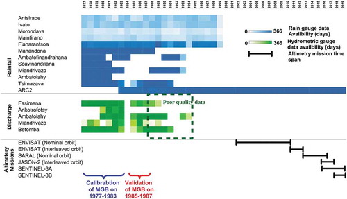
For all of these altimetry missions, the high-rate data at 20 or 40 Hz are used. The timeline of each mission is shown in Fig. 3.

4.3 Meteorological data

Daily meteorological data from rain gauges and synoptic stations obtained from the Direction Générale de la Météorologie (DGM) of Madagascar are used. Their locations and temporal windows are shown in Figs 1 and 3, respectively. As far as the synoptic stations (Antsirabe, Ivato, Morondava and Maintirano) are concerned, it should be noted that the data used in this study last until 1999. In addition, rainfall data have the fewest gaps compared with data for other variables, such as humidity, pressure, wind speed and temperature.

Figure 3. Temporal data availability. For rainfall and discharge, it is counted in number of days having data per year. The brighter the colour of a block is, the fewer the available daily data from the corresponding year. MGB and ARC2 stand for Modelo de Grandes Bacias and African Rainfall Climatology 2.0, respectively

In addition to rain gauge data, daily rainfall estimates delivered by the Climate Prediction Center of the NOAA National Weather Service, specifically that of the African Rainfall Climatology ARC 2.0 product (Novella and Thiaw 2013), are also used to feed the hydrological model. This product is gridded at 0.1° spatial resolution and spans from 1983 to the present. The missing rainfall values in ARC2 are replaced by rain gauge-interpolated values using the IDW method.

Due to the gaps in the datasets of the synoptic stations, climatology is not computed from the synoptic station data. Instead, the climate normals of 1961–1990 from these synoptic stations and proposed by the World Meteorological Organization (WMO) are used. In addition, the monthly mean of the satellite-based albedo and the monthly mean of the LAI distributed by the ESA GlobAlbedo project (Muller et al. 2011) are computed and used as climatology.

4.4 Hydrological data

Daily discharge from historical hydrological stations obtained from the DGM of Madagascar are used. Their locations and time spans are shown in Figs 1 and 3, respectively. Moreover, we installed our own project gauge at Behoro village, approximately 8 km upstream from VS ENV-T0040, on the Tsiribihina River in August 2015 (Fig. 1). A discharge measurement and a cross-sectional geometry were measured during installation.

We performed the calibration of the MGB model on the period 1977–1983 and the validation on the period 1985–1987. This split is encouraged by the availability of data counted in terms of the number of days of the year for which there is data, as indicated by the colours of the blocks in Fig. 3.

5 Results and discussion

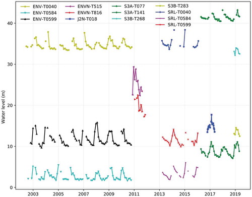
The calibration and validation of the MGB model are given in Appendix A. Similarly, the naming of the VSs and the establishment of the altimeter water levels are given in Appendix B. The locations of the VSs found along the Tsiribihina River are shown in Fig. 4. Here, the modelled discharge and water level time series along the Tsiribihina River are exploited for the computation of the RCs which in turn allow the transformation of modelled discharge or water levels into depths at the VSs.

Figure 4. Location of potential virtual stations along the Tsiribihina River from various past and actual altimetry missions, including those of SENTINEL-3 A and B, JASON-2 missions and swath coverage (pink bands) of the future SWOT mission on the Calibration/Validation or Cal/Val orbit. ENV means ENVISAT on the nominal orbit; SRL means SARAL on the nominal orbit; ENVN means ENVISAT on the interleaved orbit; J2N means JASON-2 on the interleaved orbit; and S3A and S3B mean SENTINEL-3 A and B, respectively

5.1 Rating curves

Relatively long time series of water levels were obtained from the ENVISAT mission alone at ENV-T0040, ENV-T0599 and ENV-T0584 (see Appendix B, Fig. B2). Therefore, we computed only the RCs using ENVISAT water levels at these VSs and modelled discharge at the corresponding elementary basins. Following the work of Paris et al. (2016), uniform prior probability density functions are chosen for the three parameters where $a\in \left[0;1000\right]$ $b\in \left[1;3\right]$ and $Z_0\in \left[minZ-10;minZ\right]$. 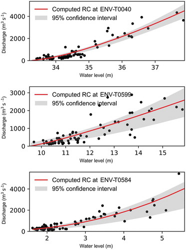For the cease-to-flow elevation $Z_0$, assuming that it should not be less than 10 m below the lowest elevation sampled by altimeter water levels ($minZ$) is a reasonable approximation for the Tsiribihina River. The parameters and quality of fit of the RCs are given in Table 1. According to the NS coefficient, the RCs at ENV-T0040 and at ENV-T0584 are of good quality (higher than 0.83) (Moriasi et al. 2007). For ENV-T0040 and ENV-T0584, the NRMSE are 7.79% and 7.26%, respectively. These values are comparable with those presented by Leon et al. (2006), Zakharova et al. (2006), Getirana and Peters-Lidard (2013) and Paris et al. (2016). For ENV-T0599, the error is higher, nearly at 16%, due to a more scattered dataset of (Z, Q) pairs. Despite the high errors found at ENV-T0599, the calculated RC is moderately good, with an NS coefficient higher than 0.5. As shown in Fig. 5, we have more points on low waters than on high waters for the three VSs. In high waters, rated discharge is affected by large uncertainties, bringing little constraint on the RC coefficients.

Table 1. Parameters and efficiency of rating curves. ENV stands for ENVISAT altimetry mission. NS and NRMSE are the Nash-Sutcliffe and the Normalized Root Mean Squared Error  efficiency coefficients

	ENV-T0040	ENV-T0599	ENV-T0584
$a$	534.61 ± 76.77	297.93 ± 62.22	94.54 ± 103.61
$Z_0$ (m)	33.27 ± 0.13	9.54 ± 0.35	0.263 ± 0.28
$b$	1.39 ± 0.11	1.17 ± 0.17	2.25 ± 0.22
NS	0.9	0.66	0.83
NRMSE (%)	7.79	15.95	7.26

Figure 5. Rating curves computed at ENV-T0040, ENV-T0599 and ENV-T0584 virtual stations using ENVISAT water levels and modelled discharge (m³ s⁻¹). RC means rating curve

The three VSs are located on the Tsiribihina River main stream with no major confluence between them. Hence, the discharge should not be significantly different from one another except for extremely high rainfall events occurring in that part of the river basin. It is shown in Appendix A that modelled discharge along this main stream was acceptable. Consequently, if we have good stage-discharge relations at ENV-T0040 and ENV-T0584 but not at ENV-T0599, we can conclude that the water level time series at ENV-T0599 has worse quality than those at the other two VSs. This may be due to the orientation of the river relative to the satellite ground tracks. The shape of the river being curved around ENV-T0599, radar echoes may not come systematically from the very location of ENV-T0599 but from a part of the river closer to the satellite (see Fig. 4 and Appendix B, Fig. B1). Under such circumstances, when it is difficult to locate with confidence the position of the reflector, correction for the water surface slope might be erroneous at ENV-T0599.

It should be mentioned that in this work, the computed RC parameters are considered stable through time. Since ENVISAT and SARAL missions use the same nominal orbit, the locations of the VSs are the same. Therefore, the RC computed at the ENVISAT VS of a given ground track can be used at the SARAL VS of the analogous ground track, noting that no RC has been computed at SARAL VSs. In the following, the RCs computed at ENV-T0040, ENV-T0599 and ENV-T0584 are used at the corresponding SARAL VSs, namely SRL-T0040, SRL-T0599 and SRL-T0584.

5.2 Depth estimation

Water depth, water level and discharge can be computed interchangeably at SRL-T0040, SRL-T0599 and SRL-T0584 using their respective RCs. In the following, the case of SRL-T0040 is discussed since estimated depths can be evaluated against Behoro gauge measurements. Here, we compare three estimates of water depth. The first depth is derived from in situ measurements by combining the readings at the staff gauge with the cross-section bathymetry collected during field work in August 2015 (Fig. 6). Second is the water depth obtained by subtracting the estimated rating curve parameter from the SARAL absolute heights. The third depth is derived by applying the inverse of the RC at SRL-T0040 to the MGB discharge series. These are presented in Figs 7 and 8.

Figure 6. Cross section at Behoro gauge measured in August 2015. Depth and elevation are given in m

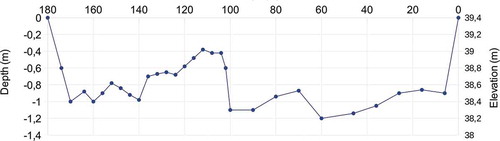
Figure 7. Time series of estimated depths (in m) at SRL-T0040 (using ENV-T0040 rating curve) and stage-derived depths (in m) at Behoro gauge (using cross-section bathymetry). SRL and ENV mean SARAL and ENVISAT, respectively

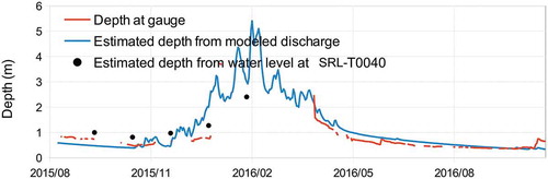
Figure 8. Scatter plot of observed depths vs. modelled discharge-derived depths and vs. SARAL water level-derived depths at SRL-T0040 (using ENV-T0040 rating curve). Dashed lines represent conventional regression lines. Depths are given in m. RMSE means Root Mean Squared Error while SRL and ENV stand for the altimetry mission names SARAL and ENVISAT, respectively

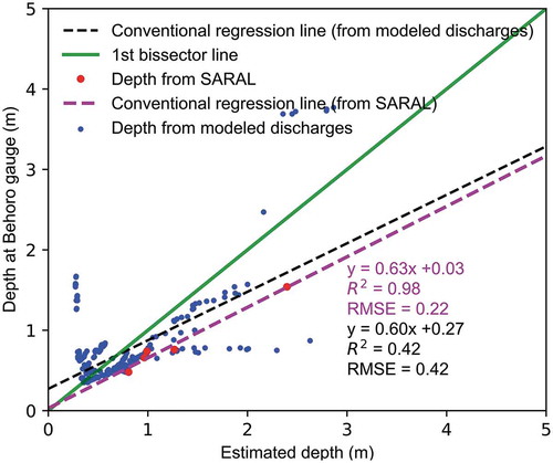
The depth series derived from the gauge and from the MGB discharge values compare very well. This good comparison provides an external validation of the RC parameters. Unfortunately, the number of SARAL measurements available for SRL-T0040 is very limited, and no definite conclusion can be drawn. However, the 0.22 m RMSE discrepancy between the gauge-derived depths and the SARAL-derived depths (thanks to the estimated RC parameter $Z_0$, which provides an estimation of the bottom elevation) suggests that satellite altimeters are promising in providing water depths even in rivers as small as the Tsiribihina River.

Due to the gap in the in situ data during high waters, depth estimation during these periods could not be evaluated properly (Fig. 7). Modelled discharge-derived depths (blue in Fig. 8) show moderately high correlation with gauge-derived depths, with the corresponding R2 being equal to 0.42. The modelled discharge-derived depths and the SARAL-derived depths show practically identical slope values of 0.6 (Fig. 8), which is confirmed by the parallelism of the corresponding regression lines. This slope, departing from a perfect value of 1.0, reflects the differences between cross-sectional geometries at SRL-T0040 and at the Behoro gauge. In fact, at SRL-T0040, the Tsiribihina River flows through a V-shaped plateau valley. The reach becomes narrower with practically a constant width compared to Behoro, where the river benefits from a large plain upper bank (see Figs 1 and 4). This explains the faster increase in depth (with a slope value less than 1) at SRL-T0040 compared to the Behoro cross section.

For the modelled discharge-derived depths, the RMSE of 0.42 m and the intercept of 0.27 m are relatively low, as they represent nearly 1/6 and 1/10 of the yearly mean depth. We can also note that the lowest modelled discharge-derived depths are practically on the 1^st bisector line (Fig. 8). These results suggest that $a,\hspace{0.17em}b$ and $Z_0$ provide plausible water depths that are well comparable with gauge measurement-derived depths.

5.3 Long-term monitoring and perspectives

The spatial organization of all the VSs relative to the Tsiribihina River can be exploited to increase temporal sampling of water level/depth/discharge estimates. Few RCs were established where long series were available (i.e. at ENV-T0040, ENV-T0599 and ENV-T0584) and showed consistency with the discharge series, while other VSs provide water level information at different locations. Here, we assume that along the Tsiribihina main reach and under low- to moderate-flow conditions, cross sections do not differ significantly along a portion of the river channel where no major confluence exists. Therefore, if a VS is relatively close to the location of another VS where a RC has been computed, a simple offset in $Z_0$ can be used to transfer water level information from the former VS to the latter (see Equation 8)(8) ${ }_{\mathrm{V}\mathrm{S}-\mathrm{V}\mathrm{S}\mathrm{r}\mathrm{e}\mathrm{f}}=\overline{Z_{\mathrm{V}\mathrm{S}\mathrm{r}\mathrm{e}\mathrm{f}}}-\overline{Z_{\mathrm{V}\mathrm{S}}}\hspace{0.17em}$(8) . In that case, the later VS is considered a reference VS (VSref). Here, the candidate VSrefs are ENV-T0040, ENV-T0599 and ENV-T0584. The offset is negative for VSs upstream of VSref and positive otherwise and is just added to each water level of a time series.

(8) ${ }_{\mathrm{V}\mathrm{S}-\mathrm{V}\mathrm{S}\mathrm{r}\mathrm{e}\mathrm{f}}=\overline{Z_{\mathrm{V}\mathrm{S}\mathrm{r}\mathrm{e}\mathrm{f}}}-\overline{Z_{\mathrm{V}\mathrm{S}}}\hspace{0.17em}$(8)

where $\overline{Z_{\mathrm{V}\mathrm{S}\mathrm{r}\mathrm{e}\mathrm{f}}}\hspace{0.17em}$ and $\overline{Z_{\mathrm{V}\mathrm{S}}}$ are the average water levels at VSref and VS, respectively. The offset ${ }_{\mathrm{V}\mathrm{S}-\mathrm{V}\mathrm{S}\mathrm{r}\mathrm{e}\mathrm{f}}$ is computed by the simple difference between the average water levels at VSref and at VS during similar hydrological years. The min/max ratio of the water levels at VS and at VSref can be used to judge whether the range of water levels being compared are similar, therefore enabling the cross-section similarity assumption. As shown in Fig. 4, we can extend the time series at ENV-T0599 with the S3A-T077 and S3B-T283 time series and at ENV-T0040 with the S3A-T141 and S3B-T268 time series. Particularly for the S3B time series, which are actually shorter than a complete hydrological year, the corresponding water levels are first transferred to the nearest S3A VS using an ${ }_{S3B-S3A}$ offset correction computed on the period of S3B and then transferred to the ENVISAT VS using an ${ }_{S3A-ENV}$ offset correction. The resulting recombined time series are shown in Fig. 9. Using the mean or the median as the average water level in the computation of the offset did not produce a major difference in the final results. In fact, the differences between the means and the medians were, on average, 0.10 m. Despite being far from ENV-T0599, the time series at J2N-T018 seems to fit correctly to the whole time series when transferred to ENV-T0599. Similarly, the time series at ENVN-T0816 and ENVN-T0515 were transferred to ENV-T0599. In Fig. 9, water level or discharge axes could also be used instead of depth axes.

Figure 9. Reconstructed multi-mission time series of depth (in $\mathrm{m}$) at ENV-T0040 (top), ENV-T0599 (middle) and ENV-T0584 (bottom). ENV means ENVISAT on the nominal orbit ; SRL means SARAL on thenominal orbit ; ENVN means ENVISAT on the interleaved orbit ; J2N means JASON-2 on the interleaved orbit; and S3A and S3B mean SENTINEL-3 A and B, respectively

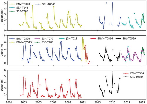
The time series in Fig. 9 can be extended into the past directly using water level information from the ERS-2 mission without any offset correction. ERS2 preceded ENVISAT and SARAL on the same orbit. By including these data, the water levels/depth/discharge could be reconstructed up to 1995.

The SWOT mission, a project of NASA and CNES, will embark the KaRIN altimeter working in interferometric SAR in the Ka band (Biancamaria et al. 2018, Morrow et al. 2018). With its wide swath, it will repeatedly provide two-dimensional maps of water level and slope at fine spatial resolution (~100 m) for rivers, lakes and floodplains. Interestingly, the orbit selected for the calibration/validation phase with a 1-day revisit time will cross the Tsiribihina River. The corresponding swath coverage is shown in pink in Fig. 4. It will provide a high-resolution longitudinal profile of rivers. Particularly for the Tsiribihina River, it will also provide a better understanding of the interaction between it and the surrounding floodplains and lakes. In return, the Tsiribihina River can be used as a validation site during this phase and to demonstrate the high potential of such a satellite mission for the monitoring of ungauged basins.

The spatio-temporal recombination of the time series of neighbouring VSs using the simple vertical offset is quite simple, but illustrates the need for long records of hydrometric data for long-term monitoring. In terms of a perspective towards the operational use of this study, we intend to use a better recombination method which is more consistent with hydraulic laws of flow propagation. Additionally, as the SENTINEL-3 A and B satellites are recent, the corresponding VSs are still active and can constitute potential reference VSs for the spatio-temporal time series recombination after computing the corresponding RCs. Moreover, the stability of the RC parameters through time and their long-term usability also should be studied. On the other hand, the major point that we will have to address in future works is about uncertainties. In this study, we used quite simple expressions to quantify uncertainties in the altimetry data and in the discharge estimates. Although we used very conservative numbers, these simplifications may affect the uncertainties associated with the rating curve parameters and with the predicted discharge. In future work, we intend to address this point more in detail. As far as MGB discharge is concerned, the way to get better estimates of the uncertainty will be to perform an ensemble of runs using perturbed parameters and inputs, or ensembles of inputs. The distribution of the discharge values simulated by the ensemble of runs will give access to more realistic uncertainties. Estimating the uncertainty specifically on each altimetry data type, instead of globally, is trickier in the absence of in situ series to compare with. Yet the refinement that we envisage in a first step is to associate a different value of uncertainty to the data coming from different missions, since the recent missions operating in SAR mode provide more accurate estimates than the old missions that used radar operated in LR mode. Lastly, we also intend to pay careful attention to the possibility of using satellite altimetry and other RS products to better constrain, a priori, the RC formulation through the verification of our hypotheses (notably the large rectangular section and constant slope hypotheses). The refined constraints will possibly lead the RC to provide discharge estimates with reduced uncertainty.

6 Conclusions

To re-initiate the hydrological monitoring of the Tsiribihina basin, this work had to face several challenges: to extract water level data from satellite altimetry over narrow river reaches, to connect historical meteorological data with rainfall products from satellites, to tune a rainfall–discharge model initially developed for large basins over a small-sized basin and establish rating curves for transforming altimeter water levels or modelled discharge into depths, and, finally, to prepend the altimetry information collected by past missions to the ones collected by the presently flying missions. The following achievements were obtained:

• The water level can be extracted successfully over narrow river reaches for the ENVISAT altimetry mission and, in a lesser proportion, from the SARAL and JASON-2 missions. Silva et al. (2010) and Becker et al. (2018) presented series over narrow river reaches. However, in both cases, it was in the favourable context of tropical forest, which bounces very little energy back to the satellite and hence produces little distortion of the echoes. Here, the Tsiribihina basin is in a more common context of rivers flowing through crops and small vegetation. This result suggests that many more water level series could be computed worldwide from these altimetry missions than observed today.

• The MGB can be tuned successfully on a small-scale river basin characterized by scarcity of in situ data in both time and space. The model is stable in using different rainfall products as input as it preserves performance on simulating discharge. This can be the case, for instance, with the transition from rain gauges to satellite-based rainfall data. This allows a continuous and long reconstruction of discharge from the oldest rain gauge data to date.

• Satellite altimeters together with hydrological modelling can be used to monitor the present-day hydrology of rivers by extending past river water level/depth/discharge fluctuations to the present. Although the satellite has a limited lifespan, long time series can be established at a given location when the satellite flies the same orbit, as in the case of the ERS-2/ENVISAT/SARAL altimetry mission series, or when another mission crosses the river nearby, as with the JASON-2 and SENTINEL-3 A and B missions.

Disclosure statement

No potential conflicts of interest were reported by the authors.

Additional information

Funding

This work was supported by the Agence Universitaire de la Francophonie and RAMI project, a regional doctoral schoolin the Indian Ocean zone, under the “Horizons Francophones” programme of the AUF (Agence Universitaire de la Francophonie).

Notes

¹ http://ctoh.legos.obs-mip.fr

² http://www.aviso.altimetry.fr

³ http://www.aviso.altimetry.fr

⁴ https://scihub.copernicus.eu

Appendix A.

Discharge modelling with the Modelo de Grandes Bacias or MGB

Figure A1 shows the spatial distribution of the twelve HRUs obtained in the Tsiribihina River basin by a combination of soil drainage potential and land-cover classes. The corresponding statistics, expressed as percentages, are given in Table A1. A total of 97% of the whole river basin is represented by five HRUs only, namely (i) medium/cropland or grassland; (ii) medium/agriculture and forest or other vegetation; (iii) medium/forest; (iv) low/cropland or grassland; and (v) low/agriculture and forest or other vegetation. This is also valid when considering each sub-catchment. Hence, to simplify the modelling, only these categories of HRUs are calibrated because the impact of other HRUs can be considered negligible.

Calibration and validation are performed per sub-catchment, from the farthest upstream to the farthest downstream to respect the runoff and stream propagation to the outlet. A comparison between the simulated (blue line) and observed (red line) hydrographs during the calibration step is shown in Fig. A2. Corresponding statistics are given in Table A2.

A comparison between the observed and simulated hydrographs during the validation step and the corresponding statistics are reported in Fig. A3 and Table A3, respectively.

The Ankotrofotsy sub-catchment could not be validated due to the limited amount of available discharge data (Fig. 3). We decided to dedicate the available 3-year discharge data to a better calibration of this sub-catchment rather than splitting the dataset in two and leaving a too-short subset of the data for validation.

The NS, NS-log and $\mathrm{\Delta }V$ efficiency criteria are reported in Tables A1 and A2. The NS values are mostly higher than 0.50 for both the calibration and the validation steps, except at Ambatolahy station, where NS takes negative values. These results suggest that high flows are modelled in an acceptable manner in four of the five sub-catchments. The NS-log values are almost all higher than 0.60, which suggests good modelling of the global range of flows, with a particular emphasis on low flows. This is confirmed by the closeness of the overall shape of the hydrographs in Figs A2 and A3, especially on the recessions. The NS-log values are also higher than the NS values, except for Miandrivazo station, with minor differences, which additionally means that seasonality and low flows are better modelled than individual peaks of high flows. Volume errors either for calibration or for validation are less than 25% for all stations except at Ambatolahy station during validation. Their negative values show that the model underestimates the discharge. Hence, according to Moriasi et al. (2007), modelling of streamflow is considered satisfactory in the Tsiribihina River basin, except for sub-catchment #3 controlled by Ambatolahy station.

Evaluating modelling performance per sub-catchment, calibration was successful in sub-catchment #4 (Ankotrofotsy station) and in sub-catchment #1 (Fasimena station). In both sub-catchments, observed hydrographs were reproduced in an acceptable manner, particularly on the recession parts, leading to good NS-log values. The NS values are slightly higher than moderate because extreme flows were somewhat underestimated, particularly in sub-catchment #1. However, the high peaks of discharge were better captured at Ankotrofotsy station than at Fasimena station, leading to a better NS value at the former (0.69 vs. 0.66) and less volume error at the former (−4.81% vs. −5.22%) (Table A2). Even if the validation attempt is preferable, we can expect that good validation performance from the upstream sub-catchment #1 is propagated to sub-catchment #4 and farther downstream to sub-catchment #5 (Betomba station). In summary, streamflow is acceptably modelled along the Mania River, except on high peaks of flow where it tends to be underestimated.

For sub-catchment #2 (Miandrivazo station), it should be mentioned that the station was re-installed at a new location in 1981 and that observations at the former location were reported by Chaperon et al. (1993) as poorly reliable. These authors reported that the ratings at the new location used to compute discharge were inaccurate and observations were often doubtful. Since no information on the confidence of each individual daily discharge value was available, we use the whole observed discharge time series. The NS-log values for simulated discharge are moderately good (see Tables A2 and A3). This suggests that the overall dynamic range of flow and particularly low flows are captured moderately along the Mahajilo River. Furthermore, the negative values for $\mathrm{\Delta }V$ suggest that the model underestimates the discharge (see Tables A2 and A3). These facts can be explained mainly by the modelled hydrograph recession shifted below the observed recession. This shift is more important in validation (Fig. A3) than in calibration (Fig. A2). The second reason is that the available rain gauges misrepresent local rainfall events, which also contributes to the underestimation of streamflow volume. In fact, many storm flow events were missed, for instance in 1982, when the rainfall values seem deficient (Fig. A2). Furthermore, the NS values are greater than the NS-log values (see Tables A2 and A3). This suggests that calibration prioritized high flows relative to moderate and low flows. We conclude that the model is better able to simulate high flows than moderate or low flows in sub-catchment #2 or along the Mahajilo.

Both manual and automatic calibrations failed in sub-catchment #3 (Ambatolahy station). Neither direct flow nor base flow could be reproduced properly (Figs A2 and A3). We performed a cross-correlation analysis between daily observed discharge at Ambatolahy station and daily areal average rainfall in sub-catchment #3 during the calibration period. Using the whole time series, the results show that there is no significant correlation (at the 5% significance level) at all (Fig. A4). This analysis highlights the poor quality of the data, whether discharge or rainfall. Chaperon et al. (1993) mentioned that the observations made at Ambatolahy station could also be of poor quality and that the sandy composition of the river margins can cause the gauge sticks to drift, which can lead to issues in the converted discharge time series. It must be noted that the inability to fine-tune the parameters is, in the present study, more likely due to the poor quality of the historical data than to the model limitations.

As shown by the calibration and validation performances at Betomba station (Tables A2 and A3), failure in modelling in sub-catchment #3 and weaknesses found in sub-catchments #1 and #4 do not significantly disturb streamflow modelling along the Tsiribihina River. In fact, the best performances are seen along this main reach, according to the three indices.

In general, the same kind of rainfall is used in rainfall–runoff modelling during calibration and validation steps. This work shows a particular case where the MGB is calibrated with rain gauge data and then run at the present time with satellite-based rainfall data. The good stability of the performance criteria (almost similar for the calibration and validation steps) suggests that the model calibrated with rain gauges can be fed with ARC2 rain data without perturbing the model performances. The key implication of this point is that daily discharge in the river basin, particularly along the main reach, except in sub-catchment #3, can be reconstructed without aberrant discontinuities or hydrological regime change artefacts from the oldest rain gauge data to present day ARC2 products, and hence to the time window of satellite altimeter data.

Appendix B.

Water level at virtual stations

The different altimetry missions used in this work provided 13 potential VSs located along the Tsiribihina River, as shown in Fig. 4. ENVISAT or SARAL nominal ground tracks intersect the Tsiribihina River at six VSs, which are labelled ENV-T0040, SRL-T0040, ENV-T0599, SRL-T0599, ENV-T0584 and SRL-T0584 from the standard labelling of the orbit passes. Note that the ENVISAT and SARAL VSs having the same orbit pass label are emplaced at the same locations. In addition, two other ENVISAT VSs, ENVN-T0816 and ENVN-T0515, which provide relatively short time series, could be established when the satellite flew on the secondary orbit. JASON-2 has only a single intersection with the Tsiribihina River at J2N-T018, which is close to the Betomba former gauging station. SENTINEL-3 A and B provide four VSs named S3A-T077, S3A-T141, S3B-T283 and S3B-T268, which interestingly bracket the four VSs ENV-T0599, SRL-T0599, ENV-T0040 and SRL-T0040. The river width is approximately 300 m along this reach.

Off-nadir measurements were observed on the altimetry measurements of the VSs and helped with the point measurement selection. We present the cases of VSs SRL-T0040, SRL-T0599 and SRL-T0584 on the left, the middle and the right, respectively, in Fig. 14. Track 040 is a descending track, i.e. the satellite flies from north to south. The altimeter “locked” its tracking of powerful echoes on the part of the Tsiribihina River flowing north–south, which is almost parallel to the satellite ground tracks (region 1, Fig. B1) until crossing (region 2, Fig. B1). We can also see that the highest values of the backscatter/retrodiffusion coefficient (${\sigma }_0$ approximately 30 dB and in orange) roughly map the course of the river. This certainly results from the advantage of using 40 Hz sampling. Even farther south, the crossing at region 2, ${\sigma }_0$ is still high, indicating that the altimeter is still “locked” on the river and still measuring its water level. In this case, the river being away from the nadir of the satellite antenna, range measurements are overestimated satellite-river distances. When looking at the along-track water level profile, the measurements in region 2 of Fig. B1 draw parabola patterns whose summits are located in the immediate vicinity of the river. These parabola patterns become an additional means for detecting valid measurements related to water together with high ${\sigma }_0$, and become advantageous for narrow rivers such as the Tsiribihina River. Although track 0040 has multiple overlaps with the Tsiribihina River, we consider only the crossing at region 2 where individual measurements draw clear parabola patterns.

Track 0599 is an ascending track. Only short portions of hooking parabolas, compared to track 0040 parabolas, were observed on every cycle, making point selection challenging (region 3, Fig. 14). The spatial distribution of high values of ${\sigma }_0$ indicates the localization of the river channel, while the gradual along-track variation of ${\sigma }_0$ correlates with a gradual increase in the distance of the altimeter measurement point from the river. In addition, finding meaningful points relative to the river at SRL-T0584 was more difficult because several water bodies are in proximity to the river. This is supported by the spread of high values of ${\sigma }_0$ inside almost all the spatial window (region 4, Fig. B1) and by the groups of dark pixels in the background image seeming to be water bodies.

Parameter ${\sigma }_0$, which measures the total energy of the echo, is used to assess how well the river was detected. For example, with SARAL/AltiKa, values in the vicinity of river/water bodies range from approximately 20 to 40 dB, as illustrated in Fig. B1. This range is comparable to the findings of Birkett (1998).

As mentioned, the actual ground track of the satellite orbit can depart from the theoretical track by a few hundreds of metres, as illustrated in Fig. B1. To bring the measurements back to the locations of the VSs, the surface slopes were derived from a longitudinal GPS profile of the Tsiribihina River performed in October 2018. Slope values are 0.56 m/km for ENV-T0040 and SRL-T0040, 0.30 m/km for ENV-T0599 and SRL-T0599, 0.02 m/km for ENV-T0584 and SRL-T0584, 0.22 m/km for S3A-T077, 0.40 m/km for S3B-T283, 0.30 m/km for ENVN-T0816, ENVN-T0515 and J2N-018, 0.60 m/km for S3B-T268 and 0.15 m/km for S3A-T141. These slope values are used to correct the vertical shift introduced by the orbit drift over time.

Because the SARAL mission uses a different ellipsoid than the one used by the other missions, SARAL heights are corrected for the difference of 70 cm between the radii of the two ellipsoids prior to projection onto EGM2008. In addition, as explained by Bosch et al. (2014), systematic bias in the ranges often affects altimeter water levels. To represent the real water surface elevation, the bias relative to each mission has to be removed. ENVISAT time series are corrected for an absolute bias of 1.044 m (Calmant et al. 2013). SARAL time series are corrected for an absolute bias of 0.263 m (Silva et al. 2015). JASON-2 time series are corrected for an absolute bias of 0.35 m (Seyler et al. 2013). SENTINEL-3 A and B time series are adjusted for an absolute bias of 0.285 m (Crétaux et al. 2018). The resulting time series are shown in Fig. B2.

In general, four to five radar measurements are used to compute individual water levels and corresponding standard deviations. These measurements were selected based on their ${\sigma }_0$ values and when they draw parabola patterns with summits falling in the immediate vicinity of the river. Specifically, for some VSs, such as ENV-T0040 and SRL-T0040, 10 points or more could be selected where long parabola patterns exist. Careful selection of high rate points for the computation of water level either for ENVISAT or SARAL permitted very low formal uncertainties, ranging from 0.01 m to 0.87 m and on average less than 0.10 m. The amplitude of the variation in the water level along the Tsiribihina River is approximately 3 m to 4 m on average (Fig. B2). These amplitudes are consistent with the seasonality of the Tsiribihina River reported by Baudin (1982) and Chaperon et al. (1993). Apparently, actual altimetry missions did not sense some extremely high-flow conditions, which is probably due to the rareness and brevity of such events and to the low temporal sampling of the altimetry missions.

Table A1. Spatial distribution of Hydrologic Response Units (HRUs) (in %). Complement means the sub-catchment downstream from Betomba

HRU class	1	2	3	4	5	6	7	8	9	10	11	12	Sum
1 – Fasimena	57.1	29.6	13.3	0.0	0.0	0.0	0.0	0.0	0.0	0.0	0.0	0.0	100
3 – Ambatolahy	49.3	49.3	0.0	0.0	0.0	1.0	0.0	0.3	0.0	0.0	0.0	0.0	100
4 – Ankotrofotsy	60.6	39.0	0.4	0.0	0.0	0.0	0.0	0.0	0.0	0.0	0.0	0.1	100
2 – Miandrivazo	81.5	15.7	0.2	0.2	0.0	0.9	0.0	0.1	0.0	0.0	0.0	1.4	100
5 – Betomba	55.6	17.3	3.3	0.4	0.4	10.1	0.4	6.6	3.2	0.0	0.0	2.8	100
6 – Complement	23.3	15.0	29.0	0.9	0.6	10.2	1.6	7.0	2.8	0.7	3.8	5.1	100
Whole basin	62.6	24.6	4.8	0.2	0.1	3.1	0.2	1.9	0.8	0.0	0.3	1.4	100

Table A2. Calibration performance statistics. NS represents the Nash-Sutcliffe coefficient. NS-log represents the NS computed on the logarithm of the discharges

Sub-catchment	Gauge	River	Drained area (km^2)	NS	NS-log	Volume error (%)
1	Fasimena	Mania	6 795	0.66	0.72	−5.22
2	Miandrivazo	Mahajilo	14 375	0.61	0.44	−10.93
3	Ambatolahy	Sakeny	1 863	−0.05	−0.85	0.01
4	Ankotrofotsy	Mania	17 990	0.69	0.74	−4.81
5	Betomba	Tsiribihina	45 000	0.76	0.84	−2.26

Table A3. Validation performance statistics. NS represents the Nash-Sutcliffe coefficient. NS-log represents the NS computed on the logarithm of the discharges

Sub-catchment	Gauge	River	Drained area (km^2)	NS	NS-log	Volume error (%)
1	Fasimena	Mania	6795	0.58	0.71	−9.96
2	Miandrivazo	Mahajilo	14375	0.55	0.49	−9.74
3	Ambatolahy	Sakeny	1863	−0.18	−2.91	−57.97
4	Ankotrofotsy	Mania	17990
5	Betomba	Tsiribihina	45000	0.72	0.85	−3.76

Figure A1. Spatial distribution of Hydrologic Responce Units (HRUs) (soil drainage potential was considered according to four ranks: hydromorph, low, medium and high) and sub-catchment numbering (bottom left)

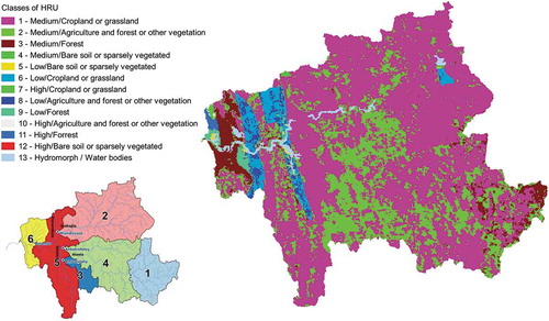
Figure A2. Comparison of observed and calculated hydrographs for the calibration step. Red lines: in situ discharge (m³ s⁻¹); blue lines: modelled discharge (m³ s⁻¹); and green lines: upstream rainfall (mm)

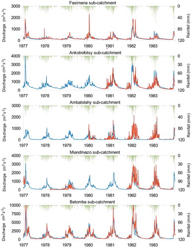
Figure A3. Comparison of observed and calculated hydrographs for the validation step. Red lines: in situ discharge (m³ s⁻¹); blue lines: modelled discharge (m³ s⁻¹); and green lines: upstream rainfall (mm)

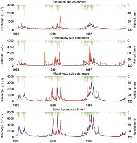
Figure A4. Cross-correlation analysis between observed discharge (m³ s⁻¹) at Ambatolahy station and average rainfall (mm) in sub-catchment #3

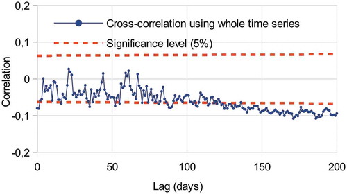
Figure B1. Along-track SARAL-AltiKa 40 Hz points showing backscatter coefficient (dB) spatial variation and along-track height (in m with respect to the WGS84 ellipsoid) variation at SRL-T0040 (left), SRL-T0599 (middle) and SRL-T0584 (right) overlain on Landsat 8 Operational Land Imager (OLI) band 5 acquired on 2 May 2014. SRL stands for SARAL

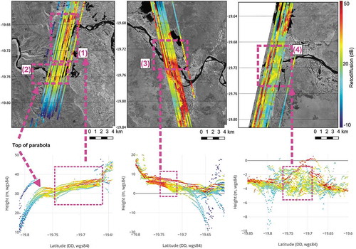
Figure B2. Altimeter water level time series at virtual stations. ENV means ENVISAT on the nominal orbit; SRL means SARAL on thenominal orbit; ENVN means ENVISAT on the interleaved orbit; J2N means JASON-2 on the interleaved orbit; and S3A and S3B mean SENTINEL-3 A and B, respectively

References

- Abdelmalik, K.W., 2016. Role of statistical remote sensing for inland water quality parameters prediction. The Egyptian Journal of Remote Sensing and Space Science, 21 (2), 193–200. doi:10.1016/j.ejrs.2016.12.002
- Allasia, D., Silva, B.C.D., and Tucci, C.E.M., 2006. Large basin simulation experience in South America. In: M. Sivapalan, et al., eds. Prediction in ungauged basins: promises and progress. Proc. Brazil Symp., April 2005. Wallingford, UK: IAHS Press, 360–370.
- Andreadis, K.M., Schumann, G.J.P., and Pavelsky, T., 2013. A simple global river bankfull width and depth database. Water Resources Research, 49 (10), 7164–7168. doi:10.1002/wrcr.20440
- Asadzadeh Jarihani, A., et al., 2013. Evaluation of multiple satellite altimetry data for studying inland water bodies and river floods. Journal of Hydrology, 505, 78–90. doi:10.1016/j.jhydrol.2013.09.010
- Bárdossy, A., 2007. Calibration of hydrological model parameters for ungauged catchments. Hydrology and Earth System Sciences, 11 (2), 703–710. doi:10.5194/hess-11-703-2007
- Baudin, D., 1982. La Tsiribihina à Betomba; Etude hydrologique. Antananarivo, Madagascar: ORSTOM.
- Becker, M., et al., 2018. Satellite-based estimates of surface water dynamics in the Congo River Basin. International Journal of Applied Earth Observation and Geoinformation, 66, 196–209. doi:10.1016/j.jag.2017.11.015
- Beven, K.J., 2001. Rainfall–runoff modeling: the primer. Chichester: John Wiley & Sons.
- Biancamaria, S., et al., 2018. Validation of Jason-3 tracking modes over French rivers. Remote Sensing of Environment, 209, 77–89. doi:10.1016/j.rse.2018.02.037
- Birkett, C.M., 1998. Contribution of the TOPEX NASA radar altimeter to the global monitoring of large rivers and wetlands. Water Resources Research, 34 (5), 1223–1239. doi:10.1029/98WR00124
- Birkinshaw, S.J., et al., 2010. Using satellite altimetry data to augment flow estimation techniques on the Mekong river. Hydrological Processes, 24 (26), 3811–3825. doi:10.1002/hyp.7811
- Bizzi, S., et al., 2015. The use of remote sensing to characterise hydromorphological properties of European rivers. Aquatic Sciences, 78 (1), 57–70.
- Bjerklie, D.M., et al., 2003. Evaluating the potential for measuring river discharge from space. Journal of Hydrology, 278 (1–4), 17–38. doi:10.1016/S0022-1694(03)00129-X
- Bodian, A., 2012. Approche par modélisation pluie-débit de la connaissance régionale de la ressource en eau : application au haut bassin du fleuve Sénégal. Physio-Géo, 6 (1), 3–5. Environ. doi:10.4000/physio-geo.2561
- Bosch, W., Dettmering, D., and Schwatke, C., 2014. Multi-mission cross-calibration of satellite altimeters: constructing a long-term data record for global and regional sea level change studies. Remote Sensing, 6 (3), 2255–2281. doi:10.3390/rs6032255
- Boughton, W. and Chiew, F., 2007. Estimating runoff in ungauged catchments from rainfall, PET and the AWBM model. Environmental Modelling and Software, 22 (4), 476–487. doi:10.1016/j.envsoft.2006.01.009
- Calmant, S., et al., 2013. Detection of envisat RA2/ICE-1 retracked radar altimetry bias over the Amazon basin rivers using GPS. Advances in Space Research, 51 (8), 1551–1564. doi:10.1016/j.asr.2012.07.033
- Castiglioni, S., et al., 2010. Calibration of rainfall–runoff models in ungauged basins: a regional maximum likelihood approach. Advances in Water Resources, 33 (10), 1235–1242. doi:10.1016/j.advwatres.2010.04.009
- Cazenave, A., et al., Eds. 2016. Remote sensing and water resources, space sciences series of ISSI. Switzerland: Springer International Publishing.
- Chaperon, P., Danloux, J., and Ferry, L., 1993. Monographie Hydrologiques de l’ORSTOM, 10. Fleuves et rivières de Madagascar. Paris: ORSTOM Direction de la Météorologie et de l’Hydrologie.
- Chen, F.-W. and Liu, C.-W., 2012. Estimation of the spatial rainfall distribution using inverse distance weighting (IDW) in the middle of Taiwan. Paddy and Water Environment, 10 (3), 209–222. doi:10.1007/s10333-012-0319-1
- Coe, M.T. and Birkett, C.M., 2004. Calculation of river discharge and prediction of lake height from satellite radar altimetry: example for the Lake Chad basin. Water Resources Research, 40 (10), W10205. doi:10.1029/2003WR002543
- Collischonn, W., et al., 2007a. The MGB-IPH model for large-scale rainfall—runoff modeling. Hydrological Sciences Journal, 52 (5), 878–895. doi:10.1623/hysj.52.5.878
- Collischonn, W., et al., 2007b. Medium-range reservoir inflow predictions based on quantitative precipitation forecasts. Journal of Hydrology, 344 (1–2), 112–122. doi:10.1016/j.jhydrol.2007.06.025
- Cosgrove, W.J. and Loucks, D.P., 2015. Water management: current and future challenges and research directions. Water Resources Research, 51 (6), 4823–4839. doi:10.1002/2014WR016869
- Coss, S., et al., 2020. Global river radar altimetry time series (GRRATS): new river elevation earth science data records for the hydrologic community. Earth System Science Data, 12 (1), 137–150. doi:10.5194/essd-12-137-2020
- Crétaux, J.-F., et al., 2018. Absolute calibration or validation of the altimeters on the sentinel-3A and the Jason-3 over lake Issykkul (Kyrgyzstan). Remote Sensing, 10 (11), 1679. doi:10.3390/rs10111679
- Cunge, J.A., 1969. On the subject of a flood propagation computation method (Muskingum method). Journal of Hydraulic Research, 7 (2), 205–230. doi:10.1080/00221686909500264
- Durand, M., et al., 2009. Estimating river depth from remote sensing swath interferometry measurements of river height, slope, and width. IEEE Journal of Selected Topics in Applied Earth Observations and Remote Sensing, 3 (1), 20–31.
- FAO, 2002. Land use-land cover map of the world made by international food policy research institute IFPRI. Rome, Italy: Food and Agriculture Organization of the United Nations.
- FAO/IIASA/ISRIC/ISS-CAS/JRC, 2012. Harmonized world soil database (ver. 1.2). Rome, Italy and IIASA, Laxenburg Austria: FAO.
- Fernandes, M.J., et al., 2014. Atmospheric corrections for altimetry studies over inland water. Remote Sensing, 6 (6), 4952–4997. doi:10.3390/rs6064952
- Fonds Africain de Développement, 1994. Rapport d’achèvement Projet d’aménagement hydro-agricole de la Tsiribihina Phase I Manambolo Madagascar.
- Fonds International de Développement Agricole (FIDA), 2013. Projet d’Appui au Développement du Melaky et du Menabe (AD2M) Rapport de supervision.
- Fonstad, M.A. and Marcus, W.A., 2005. Remote sensing of stream depths with hydraulically assisted bathymetry (HAB) models. Geomorphology, 72 (1–4), 320–339. doi:10.1016/j.geomorph.2005.06.005
- Food and Agriculture Organization of the United Nations, World Food Program, 2013. Rapport spécial mission FAO/PAM d’évaluation de la sécurité alimentaire à Madagascar.
- Frappart, F., et al., 2006. Preliminary results of ENVISAT RA-2-derived water levels validation over the Amazon basin. Remote Sensing of Environment, 100 (2), 252–264. doi:10.1016/j.rse.2005.10.027
- Frappart, F. and Marieu, V., 2015. Multi-satellite altimetry processing software (MAPS).
- Furl, C., Ghebreyesus, D., and Sharif, H.O., 2018. Assessment of the performance of satellite-based precipitation products for flood events across diverse spatial scales using GSSHA modeling system. Geosciences, 8 (6), 191. doi:10.3390/geosciences8060191
- Garambois, P.A., et al., 2017. Hydraulic visibility : using satellite altimetry to parameterize a hydraulic model of an ungauged reach of a braided river. Hydrological Processes, 31 (4), 756–767. doi:10.1002/hyp.11033
- Getirana, A.C.V., et al., 2009. Hydrological monitoring of poorly gauged basins based on rainfall–runoff modeling and spatial altimetry. Journal of Hydrology, 379 (3–4), 205–219. doi:10.1016/j.jhydrol.2009.09.049
- Getirana, A.C.V. and Peters-Lidard, C., 2013. Estimating water discharge from large radar altimetry datasets. Hydrology and Earth System Sciences, 17 (3), 923–933. doi:10.5194/hess-17-923-2013
- Gholizadeh, M.H. and Melesse, A.M., 2017. Study on spatiotemporal variability of water quality parameters in Florida bay using remote sensing. Journal of Remote Sensing & GIS, 6 (3), 1–11. doi:10.4172/2469-4134.1000207
- Gleason, C. and Durand, M., 2020. Remote sensing of river discharge: a review and a framing for the discipline. Remote Sensing, 12 (7), 1107. doi:10.3390/rs12071107
- Global Runoff Data Centre (GRDC), 2016. Global runoff data base : temporal distribution of river discharge data. Available from: http://www.bafg.de/GRDC/EN/01_GRDC/13_dtbse/db_stat.html [ Accessed 17 April 2018].
- Hansen, C.H., et al., 2017. Spatiotemporal variability of lake water quality in the context of remote sensing models. Remote Sensing, 9 (5), 409. doi:10.3390/rs9050409
- Irimescu, A., et al., 2009. The use of remote sensing and GIS techniques in flood monitoring and damage assessment: a study case in Romania. In: A. Jones, et al., eds. Threats to global water security, NATO science for peace and security series C: environmental security. Dordrecht: Springer, 167–177. doi:10.1007/978-90-481-2344-5_18
- Klemas, V., 2014. Remote sensing of floods and flood-prone areas: an overview. Journal of Coastal Research, 1005–1013. doi:10.2112/JCOASTRES-D-14-00160.1
- Kosuth, P., Blitzkow, D., and Cochonneau, G., 2006. Establishment of an altimetric reference network over the Amazon Basin using satellite radar altimetry (Topex Poseidon). Proceeding of the Symposium on 15 years of Progress in Radar Altimetry. Netherlands: ESA Publications DivisionI.
- Kouraev, A.V., et al., 2004. Ob’ river discharge from TOPEX/Poseidon satellite altimetry (1992–2002). Remote Sensing of Environment, 93 (1–2), 238–245. doi:10.1016/j.rse.2004.07.007
- Kouwen, N., et al., 1993. Grouped response units for distributed hydrologic modeling. Journal of Water Resources Planning and Management, 119 (3), 289–305. doi:10.1061/(ASCE)0733-9496(1993)119:3(289)
- Krause, P., Boyle, D.P., and Bäse, F., 2005. Comparison of different efficiency criteria for hydrological model assessment. Advances in Geosciences, 5, 89–97. doi:10.5194/adgeo-5-89-2005
- Lebecherel, L., et al., 2015. Connaître les débits des rivières : quelles méthodes d’extrapolation lorsqu’il n’existe pas de station de mesures permanentes. Comprendre pour agir. Vincennes: Onema, 26.
- Lebigre, J.-M., 1988. Le marais maritime de la Tsiribihina à Madagascar. Paysage végétal et dynamique. Bois et Forêts des Tropiques, 215, 37–60. doi:10.19182/bft1988.215.a19608
- Legleiter, C.J., 2015. Calibrating remotely sensed river bathymetry in the absence of field measurements: flow resistance equation-based imaging of river depths (FREEBIRD). Water Resources Research, 51 (4), 2865–2884. doi:10.1002/2014WR016624
- Legleiter, C.J., Roberts, D.A., and Lawrence, R.L., 2009. Spectrally based remote sensing of river bathymetry. Earth Surface Processes and Landforms, 34 (8), 1039–1059. doi:10.1002/esp.1787
- Lehner, B. and Grill, G., 2013. Global river hydrography and network routing: baseline data and new approaches to study the world’s large river systems. Hydrological Processes, 27 (15), 2171–2186. doi:10.1002/hyp.9740
- Leon, J.G., et al., 2006. Rating curves and estimation of average water depth at the upper Negro river based on satellite altimeter data and modeled discharges. Journal of Hydrology, 328 (3–4), 481–496. doi:10.1016/j.jhydrol.2005.12.006
- Lyzenga, D.R., Malinas, N.P., and Tanis, F.J., 2006. Multispectral bathymetry using a simple physically based algorithm. IEEE Transactions on Geoscience and Remote Sensing, 44 (8), 2251–2259. doi:10.1109/TGRS.2006.872909
- Maheu, C., Cazenave, A., and Mechoso, C.R., 2003. Water level fluctuations in the plata basin (South America) from TOPEX/Poseidon satellite altimetry. Geophysical Research Letters, 30 (3), 1143. doi:10.1029/2002GL016033
- Maidment, D.R., 2002. Arc hydro: GIS for water resources. Redlands, California: ESRI, Inc.
- Maillard, P., Bercher, N., and Calmant, S., 2015. New processing approaches on the retrieval of water levels in ENVISAT and SARAL radar altimetry over rivers: a case study of the São Francisco River, Brazil. Remote Sensing of Environment, 156, 226–241. doi:10.1016/j.rse.2014.09.027
- Mdee, O.J., 2015. Spatial distribution of runoff in ungauged catchments in Tanzania. Water Utility Journal, 9, 61–70.
- Moody, J.A. and Troutman, B.M., 2002. Characterization of the spatial variability of channel morphology. Earth Surface Processes and Landforms, 27 (12), 1251–1266. doi:10.1002/esp.403
- Morel, Y. and Favoretto, F., 2017. 4SM: a novel self-calibrated algebraic ratio method for satellite-derived bathymetry and water column correction. Sensors, 17 (7), 1682. doi:10.3390/s17071682
- Moriasi, D.N., et al., 2007. Model evaluation guidelines for systematic quantification of accuracy in watershed simulations. Transactions of the ASABE, 50 (3), 885–900. doi:10.13031/2013.23153
- Morrow, R., Blumstein, D., and Dibarboure, G., 2018. Fine-scale altimetry and the future SWOT mission. In: E. Chassignet, et al., eds. New frontiers in operational oceanography. Florida State, US: GODAE OceanView, 191–226. doi:10.17125/gov2018.ch08
- Muller, J.P., et al., 2011. The ESA GlobAlbedo project for mapping the earth’s land surface albedo for 15 years from European sensors. In EGU general assembly Geophysical Research Abstracts. Saarbrücken, Germany, 13.
- Novella, N.S. and Thiaw, W.M., 2013. African rainfall climatology version 2 for famine early warning systems. Journal of Applied Meteorology and Climatology, 52 (3), 588–606. doi:10.1175/JAMC-D-11-0238.1
- Office Nationale pour l’Environnement, 2017. Résumé Tableau de Bord Environnemental Région MENABE. Antananarivo, Madagascar: ONE.
- Oudin, L., et al., 2006. Dynamic averaging of rainfall–runoff model simulations from complementary model parameterizations. Water Resources Research, 42 (7), 7. doi:10.1029/2005WR004636
- Paiva, R.C.D., Collischonn, W., and Tucci, C.E.M., 2011. Large scale hydrologic and hydrodynamic modeling using limited data and a GIS based approach. Journal of Hydrology, 406 (3–4), 170–181. doi:10.1016/j.jhydrol.2011.06.007
- Pan, Z., et al., 2015. Performance assessment of high resolution airborne full waveform LiDAR for shallow river bathymetry. Remote Sensing, 7 (5), 5133–5159.
- Papa, F., et al., 2010. Satellite altimeter-derived monthly discharge of the Ganga-Brahmaputra river and its seasonal to interannual variations from 1993 to 2008. Journal of Geophysical Research, 115 (C12). doi:10.1029/2009JC006075
- Paris, A., 2015. Utilisation conjointe de données d’altimétrie satellitaire et de modélisation pour le calcul des débits distribués dans le bassin amazonien. Thesis. Université Paul Sabatier - Toulouse III.
- Paris, A., et al., 2016. Stage-discharge rating curves based on satellite altimetry and modeled discharge in the Amazon basin. Water Resources Research, 52 (5), 3787–3814. doi:10.1002/2014WR016618
- Pavelsky, T.M., et al., 2014. Assessing the potential global extent of SWOT river discharge observations. Journal of Hydrology, 519, 1516–1525. doi:10.1016/j.jhydrol.2014.08.044
- Pavlis, N.K., et al., 2012. The development and evaluation of the earth gravitational model 2008 (EGM2008). Journal of Geophysical Research: Solid Earth, 117 (B4). doi:10.1029/2011JB008916
- Post, D.A. and Jakeman, A.J., 1999. Predicting the daily streamflow of ungauged catchments in S.E. Australia by regionalizing the parameters of a lumped conceptual rainfall–runoff model. Ecological Modelling, 123 (2–3), 91–104. doi:10.1016/S0304-3800(99)00125-8
- Présidence de la République de Madagascar, 2017. Le Japon et Madagascar s’engagent. La Revue de la Présidence 36–37. Antananarivo: Présidence de la République de Madagascar.
- Pushpalatha, R., et al., 2012. A review of efficiency criteria suitable for evaluating low-flow simulations. Journal of Hydrology, 420, 171–182. doi:10.1016/j.jhydrol.2011.11.055
- Rantz, S.E., 1982. Measurement and computation of streamflow: volume 2, computation of discharge. USGPO.
- Rawls, W.J., et al., 1993. Infiltration and soil water movement. In: D. Maidment, ed. Handbook of hydrology. New York, USA: McGraw-Hill, 5.1–5.51.
- Revilla-Romero, B., et al., 2015. Filling the gaps: calibrating a rainfall–runoff model using satellite-derived surface water extent. Remote Sensing of Environment, 171, 118–131. doi:10.1016/j.rse.2015.10.022
- Rodríguez, E., Durand, M.T., and Frasson, R.P., 2020. Observing rivers with varying spatial scales. Water Resources Research, 56 (9). doi:10.1029/2019WR026476
- Rostom, N.G., et al., 2017. Evaluation of Mariut Lake water quality using hyperspectral remote sensing and laboratory works. The Egyptian Journal of Remote Sensing and Space Science, 20, S39–S48. doi:10.1016/j.ejrs.2016.11.002
- Roux, E., et al., 2010. Producing time series of river water height by means of satellite radar altimetry - a comparative study. Hydrological Sciences Journal, 55 (1), 104–120. doi:10.1080/02626660903529023
- Schumann, G.J.-P., 2015. Preface: remote sensing in flood monitoring and management. Remote Sensing, 7 (12), 17013–17015. doi:10.3390/rs71215871
- Seyler, F., et al., 2013. From TOPEX/Poseidon to Jason-2/OSTM in the Amazon basin. Advances in Space Research, 51 (8), 1542–1550. doi:10.1016/j.asr.2012.11.002
- Sichangi, A.W., et al., 2016. Estimating continental river basin discharges using multiple remote sensing data sets. Remote Sensing of Environment, 179, 36–53. doi:10.1016/j.rse.2016.03.019
- Silva, J.S., et al., 2010. Water levels in the Amazon basin derived from the ERS 2 and ENVISAT radar altimetry missions. Remote Sensing of Environment, 114 (10), 2160–2181. doi:10.1016/j.rse.2010.04.020
- Silva, J.S., et al., 2015. The question of the AltiKa/Ice-1 bias over rivers. In EGU general assembly conference abstracts. Vol. 17. Vienna, Austria.
- Stewart, B., 2015. Measuring what we manage – the importance of hydrological data to water resources management. In: Proceedings of the international association of hydrological sciences. Presented at the hydrological sciences and water security: past, present and future - 11th kovacs colloquium 16– 17 June 2014, Paris, France: Copernicus GmbH, 80–85. doi:10.5194/piahs-366-80-2015
- Tarpanelli, A., et al., 2013. River discharge estimation by using altimetry data and simplified flood routing modeling. Remote Sensing, 5 (9), 4145–4162. doi:10.3390/rs5094145
- Todini, E., 1996. The ARNO rainfall—runoff model. Journal of Hydrology, 175 (1–4), 339–382. doi:10.1016/S0022-1694(96)80016-3
- Tourian, M.J., Schwatke, C., and Sneeuw, N., 2017. River discharge estimation at daily resolution from satellite altimetry over an entire river basin. Journal of Hydrology, 546, 230–247. doi:10.1016/j.jhydrol.2017.01.009
- Tourian, M.J., Sneeuw, N., and Bárdossy, A., 2013. A quantile function approach to discharge estimation from satellite altimetry (ENVISAT). Water Resources Research, 49 (7), 4174–4186. doi:10.1002/wrcr.20348
- Twele, A., et al., 2016. Sentinel-1-based flood mapping: a fully automated processing chain. International Journal of Remote Sensing, 37 (13), 2990–3004. doi:10.1080/01431161.2016.1192304
- US Geological Survey (USGS), 2000. Shuttle radar topography mission (SRTM) 1 Arc-second global. doi: 10.5066/F7PR7TFT
- Van Emmerik, T., et al., 2015. Predicting the ungauged basin: model validation and realism assessment. Frontiers in Earth Science, 3. doi:10.3389/feart.2015.00062
- Vrugt, J.A., et al., 2003. A shuffled complex evolution metropolis algorithm for optimization and uncertainty assessment of hydrologic model parameters. Water Resources Research, 39 (8), 1201.
- Wingham, D.J., Rapley, C.G., and Griffiths, H., 1986. New techniques in satellite altimeter tracking systems. Dig. - Int. Geosci. Remote Sens. Symp. IGARSS. Available from: http://discovery.ucl.ac.uk/1535543/ [ Accessed 30 January 2018].
- World Water Assessment Programme, 2009. The united nations world water development report 3: water in a changing world (Two Vols.). London: Routledge.
- World Wide Fund, 2011. Deuxième phase: potentiel de production d’agrocarburant durable de Madagascar; Troisième phase: besoins en agrocarburant à l’échelle nationale et les opportunités à l’exportation. Antananarivo, Madagascar:World Wide Fund.
- Yapo, P.O., Gupta, H.V., and Sorooshian, S., 1998. Multi-objective global optimization for hydrologic models. Journal of Hydrology, 204 (1–4), 83–97. doi:10.1016/S0022-1694(97)00107-8
- Yoon, Y. and Beighley, E., 2015. Simulating streamflow on regulated rivers using characteristic reservoir storage patterns derived from synthetic remote sensing data. Hydrological Processes, 29 (8), 2014–2026. doi:10.1002/hyp.10342
- Young, A.R., 2006. Stream flow simulation within UK ungauged catchments using a daily rainfall–runoff model. Journal of Hydrology, 320 (1–2), 155–172. doi:10.1016/j.jhydrol.2005.07.017
- Zakharova, E.A., et al., 2006. Amazon river discharge estimated from TOPEX/Poseidon altimetry. Comptes Rendus Geoscience, 338 (3), 188–196. doi:10.1016/j.crte.2005.10.003