Geostatistical and deterministic methods for rainfall interpolation in the Zayandeh Rud basin, Iran

ABSTRACT

A new approach to select a model for fitting to a seasonal daily average rainfall semi-variogram was developed in this study by interpolating rainfall using geostatistical methods. Using two deterministic algorithms (Thiessen polygon, THI and inverse distance weighting, IDW) and two geostatistical algorithms (ordinary kriging, ORK and universal kriging, UNK) based on a rain gauge network, a 20-year daily and annual rainfall time series was generated for the Zayandeh Rud Dam Basin (Isfahan, Iran). Seven models were fitted to the experimental semi-variogram. Evaluation criteria – root mean square error (RMSE) and correlation coefficient (R) – identified that the Gaussian model is the best fit to the experimental semi-variogram. The ORK and UNK algorithms performed better in generating data when network sizes of 27, 15 or 10 gauges were used, whereas THI produced better results at a network size of five gauges. The results show that increasing the number of gauges does not necessarily produce better estimates, and stochastic methods are more sensitive than deterministic algorithms to network size.

KEYWORDS:

• rainfall interpolation
• deterministic
• geostatistics
• Zayandeh Rud Dam Basin
• Iran
• kriging

Editor S. Archfield; Associate editor K. Soulis

1 Introduction

Climatological variables, especially precipitation, vary significantly both temporally and spatially. This variability affects hydroclimatic agricultural research regarding streamflow simulation, extreme events analysis, drought prediction, etc. (Zhang and Srinivasan 2009, Teegavarapu et al. 2018). Hydrologists are often required to estimate rainfall – a key parameter – at specific sites, using only measurements recorded at surrounding locations. In this situation, the presence of fewer rainfall stations increases the uncertainty of estimation and, consequently, increases the level of error and uncertainty in hydrologic model outputs (e.g. runoff volume, time shift of hydrographs, sediment delivery and nutrient yield) (Faurès et al. 1995, Chaubey et al. 1999). Furthermore, territorial precipitation data is also key to providing accurate flood and erosion risk maps (Syed et al. 2003, Nyssen et al. 2005, Angulo-Martínez et al. 2009). This variability in climatic parameters can be partially quantified using point data collected from irregularly distributed rain gauges. Although increasing the number of point data sources provides a better representation of climatic conditions, it also increases associated costs. This highlights the need for interpolation methods which can address the problem of spatially limited climatic data.

Data estimation for non-recorded points using surrounding points is termed interpolation (Burrough et al. 1998). Interpolation techniques are typically divided into two broad classes: deterministic and geostatistical algorithms. The most frequently employed deterministic methods are the Thiessen polygon (THI) and inverse distance weighting (IDW). While long used and initially quite simple (Paulhus and Kohler 1952), interpolation methods have now been greatly improved and are employed in nearly every field of geoscience, especially soil science (Medhioub et al. 2019, Lee et al. 2019a, 2019b), as well as having a rich history in climate-related fields (Paulhus and Kohler 1952, Willmott and Wicks 1980). While geostatistics is a long-standing discipline involving earth sciences and mathematical algorithms (Willmott and Wicks 1980, Ly et al. 2011), its use in the estimation of precipitation is more recent, emerging only in the last 20 to 30 years. The results and conclusions of some recent studies employing these interpolation techniques are listed below.

Implementing THI, IDW, spline functions (SPL) and polynomial methods for rainfall interpolation, Ball and Luk (1998) found that SPL was the most suitable. In another study (Bostan et al. 2012), five interpolation methods – multiple linear regression (MLR), ordinary kriging (ORK), regression kriging (RK), universal kriging (UNK) and geographically weighted regression (GWR) – were used to map mean annual precipitation, with the UNK and GWR methods providing the highest and lowest accuracy, respectively. Amini et al. (2019) applied different deterministic and geostatistical algorithms to simulated precipitation and temperature over the Zayandehrud basin, Iran. Based on their average monthly comparison, ORK performed better for estimating T_min while Natural Neighbor (NN) was recommended for interpolating T_max and precipitation. In a study using seven models to estimate monthly precipitation for the state of Pernambuco, Brazil, Da Silva et al. (2019) ranked first the trend surface method followed by natural neighbour, IDW and kriging methods. Wang et al. (2014) referred to local polynomial interpolation (LPI) as the best method among all applied methods to estimate precipitation over Ontario, Canada. Zhang et al. (2018) compared and evaluated interpolated gauge and gridded rainfall data for the state of Florida, USA. They introduced IDW and ORK as best interpolation algorithms in predicting daily rainfall. Jacquin and Soto-Sandoval (2013) evaluated the applicability of kriging with external drift (KED) and the optimal interpolation method (OIM) for interpolation of monthly precipitation in the data-sparse region of Aconcagua River, Central Chile. They observed a better performance of OIM than KED for the precipitation interpolation.

Predicted values obtained through interpolation methods can be very inaccurate, either greatly overestimating or underestimating a random variable such as precipitation. For example, in a study that used a circular model to produce seasonal rainfall data (Van De Beek et al. 2011), the kriging method generated negative output values for some outlier rainfall data. In another study, Kendall’s tau was used within the Markov chain Monte Carlo (MCMC) method to estimate variogram robustly for rainfall interpolation in Africa (Lebrenz and Bárdossy 2017). The study noted two solutions to overcome this problem: (a) the Deutsch method (1996), in which all negative values are given a value of zero, and (b) a model fitted to a semi-variogram that is modified to avoid negative values. As attested by a number of studies (Nalder and Wein 1998, , Chen and Liu 2012), determining the optimum number of stations to be used in interpolation processes is critical to generate accurate data. While many previous studies have focused solely on generating precipitation estimates at monthly or annual time scales (Hevesi et al. 1992, Goovaerts 2000, Price et al. 2000, Marquínez et al. 2003, Zhang and Srinivasan 2009) and in light of the fact that a change in the time step over which estimation is made will alter its reliability, few studies have addressed the use of geostatistics in estimating daily rainfall (Beek et al. 1992, Ly et al. 2011). However, certain hydrological events, such as flash flooding, are directly dependent on daily rainfall, which places a greater emphasis on its spatial resolution.

In a pair of studies, investigators attempted to ascertain the effect of network size on interpolation algorithm technique outputs. Interpolating hourly data using either kriging or a multi-quadratic method, Borga and Vizzaccaro (1997) found the former method to work better at low network densities, while the latter performed better in higher density networks. Ly et al. (2011) used THI, IDW, ORK and UNK, along with KED and ordinary cokriging (OCK) methods, to predict rainfall under different station densities (70, 40, 30, 20, 8 and 4 stations). Given their lower root mean square error (RMSE) values, the IDW and ORK methods were selected as suitable procedures, while THI was the worst method and was rejected. Contemporary computation capacity allows for the identification of the weaknesses, strengths and reliability of various methods by comparing different techniques in relation to rain gauge density. In another study, Gundogdu (2017) also suggested the ORK method as the best for rainfall interpolation based on 268 stations in Turkey, compared to inverse square distance (ISD) and linear regression. The advantage of ORK was also shown for the Hawaiian Islands by Frazier et al. (2016), using a large number of rainfall stations. Compared to these studies with a relatively high number of stations, Kumari et al. (2017) showed that the co-kriging outperformed ordinary kriging for rainfall interpolation using 80 stations in the mountainous region of Central Himalayas, India.

Despite the importance of having an adequate number of gauges to accurately generate rainfall data and make informed decisions regarding the management of water resources, developing countries like Iran often possess an inadequate number of gauges. While few such studies have been undertaken in Iran, both Assakereh (2004) and Azizi et al. (2009) noted a strong dependency between elevation and the amount of precipitation throughout most of the country, especially in mountainous areas. Accordingly, the purpose of the present study was to evaluate the performance of different deterministic and geostatistical algorithms in generating daily and annual rainfall data under different rain gauge station network sizes for Iran’s Zayadeh Rud Dam basin. The results of this research will be of interest to climatologists, hydrologists and decision makers. The remainder of this paper is organized into a methodology section, a results section and a discussion section. The methodology section identifies the study area and different interpolation algorithms used for precipitation estimation. The results of the application of different interpolation methods for predicting daily and annual precipitation under different rain gauge station network sizes are presented in the results section. The discussion serves to analyse the results and to present the authors’ conclusions and suggestions.

2 Study area and data

Situated in the western portion of the Zayandeh Rud basin (Isfahan province, Iran) and extending over an area of 4087.8 km² (32°11ʹ54ʹʹ–33°11ʹ32ʹʹN, 50°2ʹ43ʹʹ–50°46ʹ27ʹʹE), the Zayandeh Rud Dam Basin slopes generally downward from northwest to southeast, with a maximum elevation of 3295 m in the southwest mountainous region and a minimum elevation of 2010 m at the basin outlet where the Zayandeh Rud (Chadegan) dam is located (Fig. 1). Precipitation in the basin is predominantly affected by rainfall systems originating in the Mediterranean Sea, which enter the country from the northwest. Rainfall decreases rapidly across the basin: from almost 1200 mm year⁻¹ on the uppermost portions of the catchment to the northwest and southwest, down to nearly 600 mm year⁻¹ in the central portion and close to 200 mm year⁻¹ at the dam’s location in the east. Over 89% of the precipitation events occur between November and March, with an annual average of 70 rainy days. According to the Dumartan climate classification, the catchment can be classified as harbouring a cold climate (Morid 2003). The Dumartan climate classification also includes an aridity index based on precipitation and temperature: the six climate classes Arid, Semi-arid, Mediterranean, Semi-humid, Humid and Hyper-humid exist within the basin (Tabari et al. 2014).

Like rainfall, annual mean temperature varies with elevation, from 6°C in the mountains of the northwest and southwest to 10°C at the Zayandeh Rud Dam; however, in the mountainous Kohrang region of the basin’s southwestern portion (Fig. 1), it can fall below −15°C in the winter. Most runoff originates from the mountains surrounding the basin, particularly in the Zagros Mountain range and Kohrang region (Morid 2003). This basin was selected not only because it is a region with varying climatic conditions (from arid to wet), but also because it is instrumented with more rain gauges than other basins: a very important element for generating accurate data interpolations.

Figure 1. Zayandeh Rud Dam Basin, Iran, showing all existing rain gauges located inside and outside the basin (black points) and the three validation stations (red points)

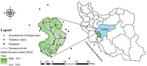
Figure 2. Three network sizes of (a) 15, (b) 10 and (c) 5 rain gauges

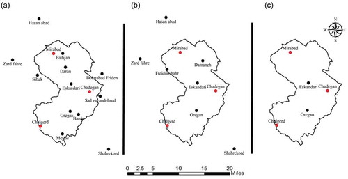
Figure 3. Dendrogram for all selected stations with cutting line (in red) at a distance of 2.5 mm

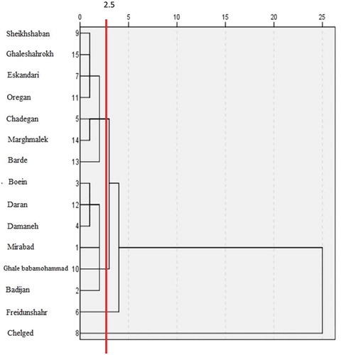
Figure 4. General flow chart of the research method

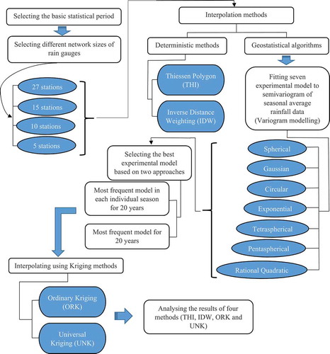
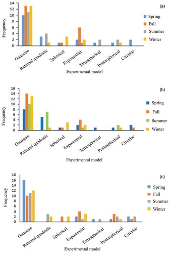
Figure 5. Number of fitted experimental models (seven models) to the semi-variogram for each season. The semi-variogram is based on seasonal average rainfall. (a) Chelgerd, (b) Chadegan and (c) Mirabad

Data from 27 rain gauge stations in and around the Zayandeh Rud Dam basin, including 18 maintained by the Ministry of Energy (Iran) and nine by the Iran Meteorological Organization (IRIMO), were used in the present study. Further characteristics of these gauges are shown in Table 1. Precipitation records extended from 20 to over 35 years depending on the station from which they originated. Daily rainfall data for the 20-year period from 21 September 1992 to 21 September 2012 was selected as the common statistical period for all climatic stations so that all existing gauges could be used in the interpolation process (Fig. 1).

Table 1. Characteristics of different gauges maintained by the Ministry of Energy and Iran Meteorological Organization (IRIMO)

No.	Gauge name	Elevation(m)	Longitude (degree-minute)	Latitude (degree-minute)	Annual mean (mm year^−1)	Related organization
1	Badijan	2300	33-04	50-20	496.83	IRIMO
2	Ghale babamohammad	2300	33-16	50-41	335.33	Ministry of Energy
3	Boien	2449	33-03	50-10	321.32	Ministry of Energy
4	Ghale shahrokh	2080	32-39	50-27	390.31	Ministry of Energy
5	Marghmalek	2470	32-47	50-50	341.33	Ministry of Energy
6	Marde	2380	32-34	50-31	340.86	Ministry of Energy
7	Shekh shaban	2300	32-53	50-36	391.64	Ministry of Energy
8	Oregan	2221	32-35	50-25	426.29	Ministry of Energy
9	Daran	2290	32-58	50-22	309.56	IRIMO
10	Ashen	2243	33-05	50-41	197.86	Ministry of Energy
11	Fereidun shahr	2490	32-58	50-22	495.55	IRIMO
12	Eskandari	2172	32-49	50-26	368.45	Ministry of Energy
13	Mirabad	2540	33-08	50-23	302.41	Ministry of Energy
14	Chelgerd	2400	32-45	50-12	1316.44	Ministry of Energy
15	Chadegan	2100	32-46	50-37	298.18	IRIMO
16	Zard fahre	2447	33-00	49-48	565.74	Ministry of Energy
17	Hasan_abad	2070	33-22	50-04	394.59	Ministry of Energy
18	Dolatabad Friden	2300	32-55	50-45	298.50	Ministry of Energy
19	Ghale nazer	2209	32-59	50-49	283.45	Ministry of Energy
20	Sibak	2552	32-53	50-04	463.12	Ministry of Energy
21	Pol zamankhan	1860	32-29	50-23	307.60	IRIMO
22	Sad zayandehrud	2173	32-43	50-44	223.90	Ministry of Energy
23	Shahrekord	22061	32-20	50-51	298.09	IRIMO
24	Kohrang	2330	32-18	50-51	1214.30	Ministry of Energy
25	Golpaigan	1870	33-28	50-16	229.60	IRIMO
26	Damane	2300	33-01	50-48	348.11	IRIMO
27	Meyhe	2500	32-24	50-21	513.57	Ministry of Energy

2.1 Density of the station network

Although it is often believed that a greater number of stations produce more accurate interpolation results, this is not always the case (Chen and Liu 2012). It is worth noting that the optimal number of spatial points required for a satisfactory interpolation depends on the number and distribution of the sample points. In instances of spatially variant precipitation, an estimation using an evenly distributed pattern (considering all the prediction space) of fewer points is more accurate than an estimation based on a greater number of unevenly distributed points (considering just some parts of the prediction space) (Johnston et al. 2001, Yao et al. 2013). Accordingly, the present study focused on using different numbers (5, 10, 15 and 27) of gauging sites (network sizes) to evaluate their function in the interpolation process and to investigate whether it is possible to obtain accurate results using fewer gauges. One solution is to consider sufficient points to achieve a representative sample. The first network size includes all 27 existing rain gauges, while other network sizes were created following a systematic process that accounts for the fact that precipitation is a function of spatial features including elevation, longitude and latitude. The 27 stations were separated into individual groups according to the similarity of their spatial features, and some stations from each group were eliminated to create a network size of 15 gauges. These processes were repeated to achieve station densities of 10 and five (Fig. 2).

2.2 Interpolation methods

The interpolation process for a specific station was undertaken using the surrounding points. The measured values closer to the prediction location have a greater influence on the predicted value than do those farther away. In fulfilling the simulation process through all interpolation procedures, the passive point (unmeasured point) is left out and its value is predicted using surrounding points. The main formula for interpolation is given as follows (Rendu 1978):

(1) $Z_{s_0}=\sum _{i=1}^{i=n}{\lambda }_i.Z_{s_0}$(1)

where $Z_{s_o}$ is the amount of rainfall at a non-measured point (mm), $Z_{s_i}$ is the amount of rainfall at specific station i and ${\lambda }_i$ is an indefinite weight for the measured rate at station i, which can be estimated through different methods (Krige 1994).

The problem lies in calculating the weights, ${\lambda }_i$, as different methods compute various weights to be used in interpolation. As the purpose of this study was to evaluate the performance of different simple and complex methods, a discussion of different interpolation methods follows (sections 2.4.1 and 2.4.2). In this study, passive points represent all the stations situated in the centre of a 400-m default grid for the data generated by ArcGIS (v. 10.1, Esri, Redlands). Given the greater spatial variability in the mountainous portions of the basin, this grid size is small enough to be representative of a zone of homogeneous precipitation. ArcGIS software was used to automatically perform all the calculations (from calculating semi-variograms to the interpolation methods) in this study.

2.2.1 Deterministic methods

These prediction methods are directly based on the surrounding measured values or on specified mathematical formulas that determine the smoothness of the resulting surface. Deterministic interpolation techniques create surfaces from measured points, based on either the extent of similarity (inverse distance weighted) or the degree of smoothing (radial basis functions). The two most well-known methods are THI and IDW.

2.2.1.1 Thiessen polygon (THI).

The THI method divides the surface of the basin into polygons such that each polygon bears the same number of variables (i.e. rainfall) throughout (Chow 1964). Every interpolated point receives its rainfall depth from the closest station. Therefore, the accuracy of interpolation from this method is largely dependent on gauge density. The advantage of this procedure is its simplicity and the possibility of making an estimation based on a single station; however, this method is prone to sudden changes in the value of predicted variables from one polygon to another.

2.2.1.2 Inverse distance weighing (IDW).

IDW estimates values at non-sampled points by calculating a weighted average of observed data at surrounding points. The principal idea behind the IDW approach is that stations with greater proximity to one another will have similar records of data. Thus, the nearest point to the ungauged station plays the most important role in determining the value of the variable at the unmeasured gauge. Spatial dependency of data can be identified using the power of reverse distance (α), namely using the inverse of the distance between an active station and passive station. The significance of known points on the interpolated values, reflecting their distance from the output point, can be handled using a power parameter. A higher power value causes more proximal points to more strongly influence the estimation of an unknown point, while a lower power value attributes a greater role to proximal points that are farther away.

A power value of α = 2 has been recommended in a number of studies (Goovaerts 2000, Lloyd 2005, Ly et al. 2011) and was adopted in the present study. Stations weights were then calculated as follows (Krige 1994):

(2) ${\lambda }_1=\frac{{\sum }_{i=1}^{i=n}{\left|D_i\right|}^d.{\lambda }_i}{{\sum }_{i=1}^{i=n}{\left|D_i\right|}^d},d>0$(2)

where $\left|D_i\right|$ is the absolute distance between measured and unmeasured points, d is the impression of spatial dependency, ${\lambda }_1$ is the weighted value at the non-gauged point and ${\lambda }_i$ is the value at the i^th gauged station.

2.2.2 Geostatistical algorithms

Originally developed to predict probability distributions for particle-size-based ore grading during mining operations (Krige 1994), geostatistics is a branch of statistics closely related to interpolation methods. Creating and measuring spatial dependency (variography) among data is achieved by using an empirical semi-variogram diagram. Geostatistics focuses on spatial or spatiotemporal datasets, but extends far beyond simple interpolation problems, as it takes into consideration the studied phenomenon at unknown locations as a set of correlated random variables. Geostatistical methods serve two main purposes: (a) detecting the spatial relation between stations and (b) predicting a variable’s value for ungauged points. In doing so they consider three sources of variability: (i) the correlation between spatial random variables; (ii) redundancy, i.e. whether, in the estimation of an unmeasured point, two adjacent measured points are incorrectly weighted to the same extent; and (iii) spatial continuity – the range of distance over which a random spatial variable maintains its similarity (Champigny 1992).

2.2.2.1 Semi-variogram (variogram) modelling.

In considering these three sources of variability, the experimental semi-variogram constitutes a discrete function that allows one to calculate the level of spatial dependency between pairs of points separated by the various distances (lags) over which the variogram is calculated. For instance, lags may be calculated for samples that are 10 m apart, then for samples that are 20 m apart, then 30 m apart and so on. In this example, the distance between lags is 10 m; however, points are not spaced exactly 10 or 20 m apart. Thus, the lag settings include a lag tolerance value that is typically set to half of the distance between lags. For the previous example, this means that the first lag would include all pairs of points that are between 5 and 15 m from each other. The following parameters describe every semi-variogram:

• range, $\alpha$, the distance at which the variogram differs negligibly from the sill;

• nugget, $C_0$, the height of the jump of the semi-variogram at the discontinuity at the origin;

• partial sill, C, calculated as the sill, C₁, minus the nugget; and

• sill, $C_1$, where $C_1=C_0+C$, the limit of the variogram tending to infinite lag distances.

In models with a fixed sill, $\alpha$ is the distance at which the semi-variance first reaches the sill; whereas, for models with an asymptotic sill, $\alpha$ is conventionally taken to be the distance at which the semi-variance first reaches 95% of the sill. For more information, please refer to Bilonick (1991).

The first step in spatial modelling through the use of semi-variograms is calculating the magnitude of the semi-variogram for a given distance, i.e. computing the semi-variogram value for each pair of stations at a distance h from each other, which is done as follows (Rendu 1978):

(3) $\gamma \left(h\right)=\frac{1}{2N\left(h\right)}\sum _{i=1}^{i=N\left(h\right)}{\left(Z_{S_i}-Z_{S_i+h}\right)}^2$(3)

where $\gamma \left(h\right)$ is the magnitude of the semi-variogram of distance h, N(h) is the number of pairs of data locations at a distance h apart, and $Z_{s_i}$ and $Z_{s_i+h}$ are the magnitudes of the variable at two points h distant from one another.

Once the semi-variogram is developed, the best model is fitted. Often, studies manually fit the empirical model to the semi-variogram, which is inappropriate, as this task requires a skilled expert with field information.

As a great deal of variation in weather conditions occurs over a 20-year period, it is not logical to fit the models to a semi-variogram based on 20-year mean rainfall values across all rain gauges because these mean values do not adequately represent temporal variations in precipitation. For example, Iran experienced a severe drought episode between 1995 and 2000, which was followed by a wet period. This example illustrates why it is not recommended to use semi-variograms to fit models, as the former employs the same coefficients for wet and dry years in the interpolation process and, in doing so, fail to account for variation in precipitation. Furthermore, even at a small timescale – for example, during the drought period of 1995–2000 – mean annual values should not be used, as weather conditions may vary drastically. The objective of this study was to apply a semi-variogram model as precisely as possible, by selecting a time span with minimal spatial and temporal weather fluctuations. Previous researchers, such as Ly et al. (2011), fitted empirical models to a semi-variogram for each exceptional event. This method, however, is extremely time consuming and prompts the proposal of a new approach.

First, daily mean rainfall values for the four seasons in each year and for all existing rain gauges were calculated. The next steps used methods from previous studies and the most applicable models to this scenario. Seven models were fitted to semi-variogram diagrams using the acquired mean values in the first step.

The seven models were fitted to the above-mentioned experimental semi-variogram, resulting in seven RMSE values for each season. Subsequently, 28 RMSE values were calculated for each year and 560 values were obtained for all 20 years of interpolation for the Chelgerd station. Among the seven values of RMSE for the seven models in each season, the model with the lowest RMSE was selected as the best model. Therefore, the four best models for each year and the 80 best models for the whole 20-year period were selected. As outlined in the following section, these operations were repeated for other geostatistical algorithms and network densities, and for validation stations as well. (Figure S1 in the Supplementary material provides an example that illustrates the selected Gaussian model which performed best among all fitted models in interpolation for the Chelgerd station using 27 gauges.)

In order to enhance the accuracy of rainfall interpolation, the following two approaches for selecting the proper model are recommended:

• Selecting the best model based on it being the most frequent “best” model in each individual season for all 20 years. For this approach, the semi-variogram diagrams were obtained for the four seasons in each year based on the seasonal average.

• Model selection according to the most prevalent model for all 20 years. In this method, the model most frequently identified as the best model across all seasons was selected as the best model. Equations representing all models (spherical, Gaussian, exponential, circular, tetra-spherical, penta-spherical and rational quadratic) are given in the Supplementary material.

Following the selection of the best model, its coefficients were used to determine the weight, through equation systems of different types of kriging: e.g. ORK and UNK. For the sake of brevity, the description and formulation of these kriging methods are provided in the Supplementary material. It is worth mentioning that, to avoid negative weights using ORK and UNK, we followed the approach suggested by (Deutsch 1996), in which the negative weights are reset to zero and the remaining weights (>0) are reset to a scale between 0 and 1. In this case, the summation of weights is equal to 1, leading to unbiased estimates.

2.3 Cross-validation

In order to evaluate the performance of different interpolation methods, this study employed the cross-validation technique to directly compare the simulated and observed data for all 20 years in both annual and daily time steps, and for each season using just the daily time steps. In this process, the temporal data were discarded from the sample dataset, and the value at the same location was then estimated using the remaining samples (Isaaks and Srivastava 2001). The sample size from the validation is the number of sample data (number of existing rain gauges). However, regarding computing sources we had access to, it would be prohibitively time-consuming to generate and validate data for all gauges for all 20 years in a daily step; therefore, unlike many previous studies which randomly selected only a few validation points, this study developed a new systematic approach using a hierarchical clustering process to select the validation stations. In this clustering process, a set of stations were grouped using a distance metric (this study selected the Euclidian distance metric between daily time series of two stations) so that stations at a lesser distance fall within the same group (cluster). Therefore, a different number of groups exist at different distances (Bezdek 1974). To successfully employ the cluster analysis process, the 15 rain gauges located inside the basin were used. Since only the precipitation conditions inside the basin are important in this study, only stations located within the basin were used. While the cluster analysis process was limited to these 15 gauges, the interpolation process was not. At each network size, all existing stations were used in the interpolation process. In the study, the horizontal dendrogram, of which the horizontal axis represents the degree of dissimilarity or distance between clusters, was used for clustering. The stations were then grouped at a horizontal distance of 2.5 mm (Fig. 3) to generate the individual groups. If a scale greater than 2.6 mm had been selected, the validation points would not have been evenly distributed across the basin, leading to a misrepresentation of the precipitation values in the basin. Moreover, with a scale of less than 2.5 mm, many validation rain gauges would have been in close proximity, with similar precipitation values (e.g. Badijan and Mirabad).

In the next step, the station with the least variance in each group was selected as a validation point since its data is unlikely to contain outliers that could generate a significant error during the comparison stage. This approach was selected because the existing observed daily rainfall series of these validation rain gauges provided a large enough sample size, making interpolation easier. Also, to keep the effect of outliers on the interpolation through kriging, stations with a small variance were excluded and the stations with higher variances were kept. If the interpolation is successful using stations with high or low values, this indicates that the procedure used is suitable. The interpolated rainfalls were subsequently compared to the observed daily rainfall time series at these validation rain gauges. It should be mentioned that, as previously stated, rainfall data were generated for only three validation stations that were selected as representative of the precipitation conditions of the entire basin. To see whether the results vary if the validation points are changed, and given the time-consuming process of interpolation for each gauge, cross-validation has been executed for all gauges of each network size using interpolation by ORK.

The RMSE represents the sample standard deviation of the differences between predicted values and observed values (Hyndman and Koehler 2006) and has been used as a criterion of comparison between observed and predicted values in many contexts, including comparing interpolation methods for mapping climatic and bioclimatic variables at a regional scale in the Apennine mountains (Attorre et al. 2007) and for the spatial distribution of rainfall in the Indian Himalayas (Basistha et al. 2008). The RMSE is calculated as follows:

(4) $\mathrm{R}\mathrm{M}\mathrm{S}\mathrm{E}=\sqrt{\frac{{\sum }_{i=1}^{i=n}{\left(P_i-O_i\right)}^2}{n}}$(4)

where $O_i\mathrm{a}\mathrm{n}\mathrm{d}{P}_i$ are the measured (observed) and interpolated (predicted) values of rainfall, and n is the sample size (total days of a time series or total number of available rain gauges).

The Pearson correlation coefficient (R), a measure of the linear correlation between two variables, X and Y, was also used, as follows (Pearson 1895):

(5) $R=\frac{{\sum }_{i=1}^n\left(X_i-\bar{X}\right)\left(Y_i-\bar{Y}\right)}{\sqrt{{\sum }_{i=1}^n{(X_i-\bar{X})}^2}\sqrt{{\sum }_{i=1}^n{(Y_i-\bar{Y})}^2}}$(5)

where R is the degree of correlation between one dataset {X₁, …, X_n} containing n values and another dataset {Y₁, …, Y_n} also containing n values, and $\bar{X}$ and $\bar{Y}$ are the sample means. Figure 4 summarizes the different procedures used in this study.

3 Results

3.1 Selecting validation stations

The station with the lowest variance in its data (daily time step) among all stations of each group was selected as a validation station. Therefore, four rain gauge stations, namely Mirabad (2540 m a.s.l.), Chadegan (2100 m a.s.l.), Chelgerd (2372 m a.s.l.) and Freidunshahr (2520 m a.s.l.), with respective variance values of 14.7, 14.77, 169.8 and 32.7 mm², were selected as validation points (Table 2). Freidnunshahr was eliminated as a validation gauge due to its proximity to and similar elevation as the Mirabad station. Also, Freidnunshahr showed greater variance than Mirabad, which contributed to its elimination.

Table 2. Variance of daily rainfall for stations in different cluster groups. The validation station for each group is indicated in bold

Group number	Station name	Variance (mm^2)
1	Mirabad	14.7
	Badijan	30.6
	Boein	16.4
	Damaneh	16.2
	Ghale babamohammad	13.8
	Daran	15
2	Eskandari	18.6
	Marghmalek	17.8
	Sheykh shaban	20.2
	Chadegan	14.7
	Oregan	24.4
	Ghale shahrokh	20.2
	Bardeh	18.4
3	Chelgerd	169.8
4	Freidunshahr	32.7

Playing an important role in overall watershed discharge, Chelgerd station receives more precipitation (annual precipitation > 1100 mm year⁻¹) and shows a larger variance than other stations. Consistent with the authors’ desire for the selected control points to be spread over and cover the catchment area, this station remained in this analysis. The three selected stations benefit from having daily historical records for the past 20 years.

3.2 Model selection

Seven empirical models were fitted to semi-variograms to acquire the best-fitted model based on the lowest values of RMSE (in mm). Across all network sizes, the Gaussian model, using one of two geostatistical algorithms (ORK or UNK), displayed a better fit to the semi-variogram than the other models. In this study, 80 models with the lowest RMSE were selected among 560 models fitted to seasonal mean data. Among these 80 models, the model with the highest frequency was selected as the best model. On this basis, the Gaussian model was the best model for each season and for the entire statistical period. This is consistent with other studies (Goovaerts 2000, Ly et al. 2011) that also selected a Gaussian model as contributing to the best-fitted model (Fig. 5 and Supplementary Fig. S2). For example, Table 3 shows the RMSE value and semi-variogram components (range, nugget and sill) for the Chelgerd validation station obtained using ORK and a network size of 27 in interpolation for the four seasons of 1992.

Table 3. Performance metrics root mean square error (RMSE in mm) and the semi-variogram components (nugget and sill in mm; range in m) obtained using ordinary kriging and a network size of 27 gauges for interpolation for the four seasons of 1992 for the Chelgerd validation station. The model with the best performance is highlighted in bold

Season	Model	Range	Nugget	Sill	RMSE
Winter	Circular	116 382	0	3.54	3.98
	Spherical	132 071	0	0.96	`3.54
	Tetraspherical	132 071	0	0.88	3.86
	Pentaspherical	132 071	0	0.82	3.59
	Exponential	132 071	0	0.8	3.64
	Gaussian	96 826	0	0.98	3.45
	Rational quadratic	132 071	0	0.77	3.84
Spring	Circular	116 901	0	0.51	3.78
	Spherical	117 839	0	0.59	3.48
	Tetraspherical	155 891	0	0.53	3.99
	Pentaspherical	155 891	0	0.49	4.10
	Exponential	155 891	0	0.45	4.13
	Gaussian	97 732	0.01	0.53	3.48
	Rational quadratic	155 891	0	0.46	3.84
Summer	Circular	117 839	0	0.99	4.22
	Spherical	132 472	0	0.97	4.25
	Tetraspherical	132 472	0	0.88	4.26
	Pentaspherical	132 472	0	0.83	4.19
	Exponential	132 472	0	0.8	4.12
	Gaussian	99 320	0.01	1.02	4.09
	Rational quadratic	120 321	0	0.9	4.25
Autumn	Circular	103 265	0	0.99	3.68
	Spherical	115 487	0	0.97	3.78
	Tetraspherical	115 415	0	0.88	3.95
	Pentaspherical	116 247	0	0.83	3.54
	Exponential	119 872	0	0.8	3.67
	Gaussian	101 325	0.01	1.02	3.41
	Rational quadratic	118 745	0	0.9	3.98

3.3 Comparison of interpolation procedures

The two criteria, RMSE (in mm) and R, served to compare daily and annually observed and estimated values for the three validation stations. For Chadegan station, the value of R decreased as the number of gauges decreased, while the RMSE displayed an inverse relationship with the number of gauges. This is true for the entire study period of 20 years and for all seasons except summer. In analysing the daily results over 20 years, validation of the Chadegan station showed that ORK yielded the best results with 27 rain gauges, although the UNK and IDW lagged only slightly behind. As THI had the highest RMSE and the lowest R, it was deemed the poorest of the models. This is consistent with the annual results as well (ORK and THI as the best and worst methods, respectively) (Table 4).

Table 4. Annual R values obtained for three validation points in interpolation using different methods and network sizes. ORK (Ordinary Kriging),  UNK (Universl Kriging), IDW (Inverse Distance Weighting), THI (Thiessen)

Validation gauge	Network size	Interpolation method
		ORK	UNK	IDW	THI
Chelgered	27	0.81	0.81	0.82	0.82
	15	0.77	0.76	0.71	0.7
	10	0.74	0.8	0.81	0.81
	5	0.21	0.26	0.27	0.25
Chadegan	27	0.87	0.85	0.86	0.84
	15	0.68	0.77	0.69	0.69
	10	0.71	0.72	0.73	0.72
	5	0.02	0.05	0.02	0.72
Mirabad	27	0.82	0.83	0.79	0.78
	15	0.67	0.68	0.63	0.63
	10	0.65	0.69	0.64	0.64
	5	0.58	0.52	0.6	0.59

The four algorithms showed similar accuracies (0.7 < R < 0.8) for 27 gauges at the daily time scale; however, Both UNK and IDW generated the most accurate results in interpolation using 15 and 10 gauges (Fig. 6(a and b)). Interpolations with five gauges produced the most interesting results. In this scenario, THI (R > 0.7 for both daily and annual time scales) performed better than the other methods (R ≈ 0) (Fig. 6(a and b)). The values of RMSE and R were also calculated for all seasons.

Figure 6. RMSE and R obtained using different methods for the Chadegan station: (a) RMSE and (b) R for the 20-year period; and R for (c) spring, (d) autumn, (e) winter, and (f) summer

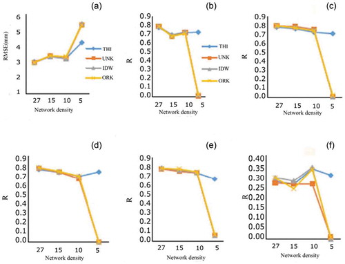
Figure 7. Observed and generated daily rainfall for three validation stations using different interpolation methods. (a) Mirabad, (b) Chadegan and (c) Chelgerd

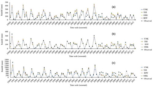
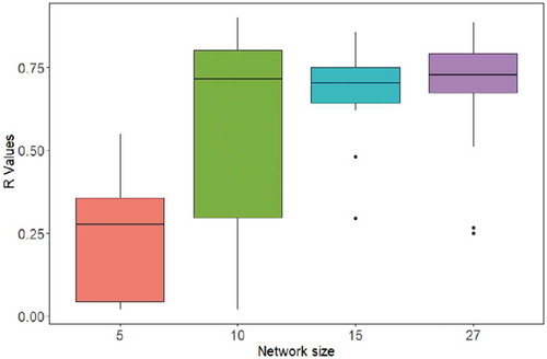
Figure 8. Boxplots of R values obtained from cross-validation for all gauges in interpolation using ORK and different network sizes

In summary, the R values obtained for the four seasons, except summer, ranged between 0.65 and 0.8 for network sizes of 27, 15 and 10 and remained higher than 0.7 for five gauges. The ORK proved to be the best model for interpolation using 27, 15 or 10 gauges, whereas the THI was the best method for interpolation with five rain gauges for the autumn and spring seasons (Fig. 6(c and d)). For winter, the best results were obtained with ORK for 27 gauges, IDW for 15 and 10 gauges, and THI (R = 0.68) for five gauges (Fig. 6(e)). The IDW was suitable for rainfall interpolation for the summer season with 27, 15 or 10 gauges, although it was outperformed, again, by the THI method for five gauges (Fig. 6(f)).

Better results were generally achieved in interpolating for the Mirabad station at both daily and annual time scales with 10 gauges rather than 15. This is true for almost all seasons. For this validation station, UNK proved to be the best algorithm, whereas for interpolation from five stations, IDW provided the most reliable results. These results were all supported by R values (Fig. S3). The annual results also support the daily results.

Based on the seasonal results, UNK was the most appropriate interpolation method when using network sizes of 27, 15 and 10 (and was among the best for five) rain gauges for the spring, autumn and winter seasons (Fig. S3). Moreover, the IDW and UNK algorithms produced more accurate results in interpolation using 27 or 15 stations than did other methods; however, ORK generated better results for 10 or five stations in the summer (Fig. S3).

In interpolation for the Chelgerd station (Fig. S4), the RMSE of daily results for the entire 20 years increased as network sizes decreased from 27 to five gauges, with the exception of a network size of 15. This is true for annual results but not for ORK. The daily results also demonstrate that IDW and THI displayed the best performance in interpolation through 27 rain gauges, which is consistent with the annual analysis, while THI produced the most acceptable results when using 15, 10 or five gauges. These results were also supported by R values (Fig. S4).

Moreover, the UNK method produced more reliable results in the interpolation of all network sizes for spring and autumn seasons, while IDW proved to be the preferred method for all network sizes for winter (Fig. S4). In interpolation for summer, THI proved the most acceptable method for network densities of 27, 15 and five gauges, while ORK was best for 10 stations (Fig. S4).

The annual mean and annual mean of maximum rainfall values were calculated based on the best-selected algorithm in interpolation across all network sizes, at both seasonal and annual time steps, for three validation gauges. These were then compared with measured seasonal and annual amounts (Table 5). For example, based on the selection of UNK as the best algorithm for interpolation using 27, 15 and 10 rain gauges and of IDW as the most reliable algorithm in interpolation using five rain gauges for the Mirabad station, the estimated annual mean rainfall using 27 rain gauges was 384 mm, compared to an observed mean value of 299 mm, and the predicted annual maximum was 45 mm, compared to the true maximum of 52 mm. Error percentages for the annual mean and annual maximum precipitation for various network sizes at three stations were calculated. The negative and positive values (Table 5) represent the percentage magnitude of underestimation or overestimation, respectively, of the interpolation algorithm.

Table 5. Observed and predicted annual mean (Mean, mm) and annual maximum mean rainfall (Max, mm) obtained by interpolation via the best method and different network sizes for Mirabad, Chadegan and Chelgerd stations for all 20 years and four seasons

Station density		20-year period		Spring		Summer		Autumn		Winter
		Measured	Estimated	Measured	Estimated	Measured	Estimated	Measured	Estimated	Measured	Estimated
					Mirabad
27	Mean	299	384 (28.4)	80	95 (18.8)	9	11 (22.2)	111	149 (34.2)	150	190 (26.7)
	Max	52	45 (−13.4)	50	45 (−10)	29	17 (−41.4)	70	45 (−35.7)	52	57 (9.6)
15	Mean	299	480 (60.5)	80	108 (35)	9	11 (22.2)	111	167 (50.5)	150	150 (0)
	Max	52	72 (38.5)	50	69 (38)	29	32 (10.3)	70	52 (−25.7)	52	74 (42.3)
10	Mean	299	495 (65.5)	80	93 (16.3)	9	7 (−22.2)	111	144 (29.7)	150	177 (18)
	Max	52	75 (44)	50	43 (−14)	29	13 (−55.2)	70	48 (−31.4)	52	68 (30.8)
5	Mean	299	540 (80.6)	80	93 (16.3)	9	7 (−22.2)	111	149 (34.2)	150	318 (112)
	Max	52	66 (27)	50	41 (−18)	29	17 (−41.4)	70	46 (−34.3)	52	103 (98.1)
					Chadegan
27	Mean	298	306 (2.6)	31	33 (6)	6	5 (−16.7)	124	125 (0)	151	157 (4)
	Max	78	62 (−25.8)	49	32 (−34.7)	35	8 (−77.1)	78	37 (−52.6)	61	62 (1.6)
15	Mean	298	298 (0)	31	32 (3.2)	6	8 (33.3)	124	118 (−4.8)	151	150 (−0.7)
	Max	78	66(−18.2)	49	29 (−40.8)	35	25(−28.6)	78	38 (−51.3)	61	62 (1.6)
10	Mean	298	303 (1.7)	31	34 (9.7)	6	5 (−16.7)	124	139 (12.1)	151	148 (−2)
	Max	78	61 (−27.9)	49	32 (−34.7)	35	8 (−77.1)	78	45 (−42.3)	61	57 (−6.6)
5	Mean	298	647 (53.9)	31	49 (58.1)	6	10 (66.7)	124	240 (93.5)	151	83 (−45)
	Max	78	103 (24.3)	49	42 (−14.3)	35	15 (57.1)	78	63 (−19.2)	61	61 (0)
					Chelgerd
27	Mean	1316	1155(−12.2)	117	79 (−32.5)	15	18 (20)	519	577 (11.2)	671	576 (−14.2)
	Max	167	220 (31.7)	87	55 (−36.8)	32	29 (−9.4)	136	220 (61.8)	179	167 (−6.7)
15	Mean	1316	1134 (−14)	117	80 (−31.6)	15	12 (−20)	489	577 (18)	671	557 (−17)
	Max	167	195 (16.7)	87	65 (−25.3)	32	22 (−31.3)	134	220 (64.2)	179	167 (−6.7)
10	Mean	1316	1171 (−11)	117	74 (−36.8)	15	18 (20)	527	577 (9.5)	671	584 (−13)
	Max	167	236 (41.3)	87	56 (−35.6)	32	29 (−9.4)	134	220 (64.2)	179	169 (−5.6)
5	Mean	1316	1151 (−12.5)	117	63 (−46.2)	15	15 (0)	438	577 (31.7)	671	540 (−19.5)
	Max	167	184 (10)	87	49 (−43.7)	32	21 (−34.4)	128	220 (71.9)	179	162 (−9.5)

Using the best interpolation algorithm across four network sizes for each validation gauge, a precipitation zonation map of annual rainfall was generated. (See Supplementary material, Fig. S5 for the rainfall distribution map for the Mirabad gauge.) Figure 7 provides a schematic comparison between aggregated seasonal time series of observed and simulated rainfall that was obtained through interpolation via 27 gauges, and the best method for each validation station. The results of interpolation and cross-validation for all gauges using ORK and different network sizes demonstrate the superiority of a gauge density of 27 while a network size of five presented the poorest results. Also, for some cases, a network size of 10 performed better than a network size of 15, whereas in other cases it did not (Fig. 8).

4 Discussion

It was assumed that in each cluster of rain gauges, the station with the lowest variance would have the least variance in its records, subsequently leading to less error in the comparison stage. This assumption held true particularly for the Chadegan and Mirabad sites compared to other stations. However, the two validation sites of Chelgerd and Freidunshahr were singles in their groups. Freidunshahr station was close to Mirabad and both time series were very similar. In order to have equally distributed validation gauges, Fereifunshahr station was subsequently discarded from the study while Chelgerd remained in use. The Chelgerd station demonstrates the effect of elevation on precipitation, as this is the area where most of the rainfall in the basin occurs. Thus, the three validation gauges used in the final evaluation process adequately represent the weather conditions of the entire basin.

Each algorithm employed in this study, from the most straightforward (THI) to the most complex (UNK), had the capacity to produce 20-year daily rainfall for the catchment grids. Results from the application of different algorithms provide insight into the strengths and weaknesses of each. Results also indicated whether deterministic and geostatistical methods were applicable to generate daily rainfall data using different densities of rain gauges in the Zayandeh Rud dam basin.

Different interpolation procedures produced similar results, except for THI, which differed most from the other methods (consistent with the results of Ly et al. 2011). Similarly, larger network sizes offered better and more homogeneous performance than the five-gauge network did. The results obtained from the daily time step study differ from those produced by the studies of Goovaerts (2000) and Lloyd (2005), which used monthly and annual time steps, and therefore cannot be directly compared.

Generally, as the number of stations increased to more than five (i.e. to 10, 15 and 27), the accuracy of the results increased, indicating a relationship between satisfactory rainfall estimation and the number of stations. According to the results, in some instances, better outputs were obtained in interpolation via 10 and 15 gauges. This difference in performance was more noticeable for geostatistical methods. Although marginally better than other network sizes, the results for 27 stations were very similar to those for 15 and 10 stations. For this reason, the optimal number of stations lies between 27 and 10. Ly et al. (2011) produced similar findings, where the use of many rain gauges (more than 10) did not improve the results significantly. In contrast, a low number of stations (five gauges) produced poor interpolation results.

It is difficult to select the best overall interpolation method, as different algorithms performed differently in interpolation for different network sizes. Based on the results, however, both ORK and UNK can be deemed the best interpolation algorithms. Frazier et al. (2016) and Zhang et al. (2018) also selected ORK as the best interpolation algorithm in comparison with other methods. The geostatistical algorithms generated better results for Chadegan and Mirabad stations because more stations were located near these two gauges than near Chelgerd. Hence, a stronger spatial dependency was created, which is crucial for better simulation via geostatistical algorithms. Consequently, poor results were obtained for the Chelgerd gauge due to its location away from other stations. The THI method performed well for Chelgerd station because, in contrast to other geostatistical methods, this method is not dependent on surrounding points. This holds true for interpolation using five gauges. Jacquin and Soto-Sandoval (2013) also obtained better estimates for gauges at high elevations using THI. Fewer gauges led to a weak spatial structure among existing stations and, consequently, poor outputs from geostatistical algorithms relative to other deterministic methods. Considerable variation in precipitation exists, both temporally and spatially. As a result, deterministic methods, especially THI, predict precipitation with low resolution, which is an insufficient representation of the rainfall conditions. Comparatively, geostatistical algorithms have higher output resolutions and produce better results. Moreover, the Thiessen polygon method ignores the pattern of spatial dependency and considers only one measurement, while IDW and geostatistical algorithms are based on the surrounding recorded values. This explains their favourable performance at the Chadegan and Mirabad stations and remains true for autumn and spring seasons, while, for summer, the reverse is true. Lebrenz and Bárdossy (2017) also referred to an increase of the quality of geostatistical methods with enhancing the dependency structure among data points. The summer season experienced less precipitation and most parts of the basin had the same amounts of rainfall. Therefore, the THI method, which creates only a few polygons, performed better in this season than did geostatistical methods. Occasionally, better results were obtained in interpolation using 10 gauges rather than 15, due to station location in relation to the target station, which influences the spatial dependency among existing gauges.

5 Conclusions

In this study, different deterministic and geostatistical methods were used to interpolate rainfall measurements in the Zavandeh Rud dam Basin in Isfahan, Iran. The performance of the different methods was compared using different network sizes. In order to select the best empirical model for fitting to a semi-variogram, a seasonal time step was first used. This method of fitting the model is more time-efficient than alternative methods.

Regarding the results of this study, although increasing the number of gauges leads to more accurate estimates, this is not true all the time and the relationship between network size and better prediction is relative. This is indicated by the results for a network size of 10 which presented more satisfactory results than a network of 15 gauges, especially in interpolation using geostatistical algorithms. This is due to the spatial structure among data points of each network size, which calculates the weight of each gauge in interpolation. A stronger spatial structure of a smaller number of gauges performs better than a weak structure with more gauges. Ly et al. (2011) obtained similar results and reached the same conclusion.

Overall, network sizes of 25 and 10 ranked first, followed by network sizes of 15 and five gauges. Similar results were obtained for Mirabad and Chadegan validation gauges, given more gauges were available surrounding them; however, as Chelged gauge is located near the border of the basin far away from other gauges and at a higher elevation than the other gauges, a strong spatial structure was not obtained and thus the performance of the deterministic methods was better than that of the geostatistical methods. This is the same in interpolation using a network size of five gauges, as a smaller number of gauges causes a very weak spatial structure among gauges, especially for the summer season because it has less rainfall than other seasons and, subsequently, a large area has the same amount of rainfall; thus, THI presents better estimates than geostatistical methods. The reverse is true for the winter season, as it includes the highest amount of rainfall and also is affected by elevation, resulting in a less homogeneous rainfall area, and in this case the THI method is not recommended for interpolation. Generally, IDW and kriging algorithms produced better results for rainfall interpolation at ungauged points, if sufficient existing gauges were present around passive points. In contrast, the THI method produced better results in a low-density network.

The interpolation methods used in this study can produce daily and annual rainfall time series with different accuracies, and this study demonstrated the possibility of obtaining more accurate results with fewer rain gauges. The agreement between the obtained results for daily and annual time scales highlights the robustness of applied interpolation methods.

This study indicates that it is possible to generate rainfall data in daily and annual time steps; however, it remains important to analyse the acquired results in different time steps, as weather parameters can vary significantly.

Upon consideration of the results of this study and the shortcomings of previous studies, the authors present the following suggestions for future studies:

• This paper used ArcGIS software for all stages of interpolation; therefore, it was impossible to create different anisotropy for each day. Thus, the same form of anisotropy was used for the entire study period. However, other software, such as Gslip, can also be used to solve this problem and could potentially lead to greater accuracy and improved speed of calculations.

• The current study focused on an area with climatic conditions ranging from semi-arid to wet. It is important to test different methods to find the best interpolation method for various climatic regions in other parts of the world, especially for arid areas where hydrological models suffer from a lack of rainfall data.

• Along with a direct comparison between generated and simulated data, another way of evaluating the generated data would be to use it as input for hydrological models, such as the Soil and Water Assessment Tools (SWAT) model (Schuol and Abbaspour 2007).

Acknowledgements

Reza Modarres would like to acknowledge support from the Center of Excellence on Risk Management and Natural Hazards, Isfahan University of Technology.

Disclosure statement

No potential conflict of interest was reported by the authors.

Supplementary material

Supplemental data for this article can be accessed here.

References

- Amini, M.A., et al., 2019. Analysis of deterministic and geostatistical interpolation techniques for mapping meteorological variables at large watershed scales. Acta Geophysica, 67 (1), 191–203. doi:10.1007/s11600-018-0226-y
- Angulo-Martínez, M., et al., 2009. Mapping rainfall erosivity at a regional scale: a comparison of interpolation methods in the Ebro Basin (NE Spain).
- Assakereh, H., 2004. Spatial changes modelling of climatic elements (Case study: annual mean precipitation of Isfahan province). Geographical researches.
- Attorre, F., et al., 2007. Comparison of interpolation methods for mapping climatic and bioclimatic variables at regional scale. International Journal of Climatology, 27 (13), 1825–1843. doi:10.1002/joc.1495
- Azizi, G., Abbaspour, R.A., Zadeh, T.S., 2009. The spatial change model at the middle mountain. Natural Geographic Researches Journal, 10, 35–51.
- Ball, J.E. and Luk, K.C., 1998. Modeling spatial variability of rainfall over a catchment. Journal of Hydrologic Engineering, 3 (2), 122–130. doi:10.1061/(ASCE)1084-0699(1998)3:2(122)
- Basistha, A., Arya, D., and Goel, N., 2008. Spatial distribution of rainfall in Indian Himalayas–a case study of Uttarakhand region. Water Resources Management, 22 (10), 1325–1346. doi:10.1007/s11269-007-9228-2
- Beek, E., Stein, A., and Janssen, L., 1992. Spatial variability and interpolation of daily precipitation amount. Stochastic Hydrology and Hydraulics, 6 (4), 304–320. doi:10.1007/BF01581623
- Bezdek, J.C., 1974. Numerical taxonomy with fuzzy sets. Journal of Mathematical Biology, 1 (1), 57–71. doi:10.1007/BF02339490
- Bilonick, R. A., 1991. An introduction to applied geostatistics.
- Borga, M. and Vizzaccaro, A., 1997. On the interpolation of hydrologic variables: formal equivalence of multiquadratic surface fitting and kriging. Journal of Hydrology, 195 (1–4), 160–171. doi:10.1016/S0022-1694(96)03250-7
- Bostan, P., Heuvelink, G., and Akyurek, S., 2012. Comparison of regression and kriging techniques for mapping the average annual precipitation of Turkey. International Journal of Applied Earth Observation and Geoinformation, 19, 115–126. doi:10.1016/j.jag.2012.04.010
- Burrough, P.A., et al., 1998. Principles of geographical information systems. Oxford: Oxford university press.
- Champigny, N., 1992. Geostatistics: a tool that works. Northern Miner, 18 May,p. 4.
- Chaubey, I., et al., 1999. Uncertainty in the model parameters due to spatial variability of rainfall. Journal of Hydrology, 220 (1–2), 48–61. doi:10.1016/S0022-1694(99)00063-3
- Chen, F.-W. and Liu, C.-W., 2012. Estimation of the spatial rainfall distribution using inverse distance weighting (IDW) in the middle of Taiwan. Paddy and Water Environment, 10 (3), 209–222. doi:10.1007/s10333-012-0319-1
- Chow, V.T., 1964. Handbook of applied hydrology; a compendium of water-resources technology.
- Da Silva, A.S.A., et al., 2019. Comparison of interpolation methods for spatial distribution of monthly precipitation in the State of Pernambuco, Brazil. Journal of Hydrologic Engineering, 24 (3), 04018068. doi:10.1061/(ASCE)HE.1943-5584.0001743
- Deutsch, C.V., 1996. Correcting for negative weights in ordinary kriging. Computers & Geosciences, 22 (7), 765–773. doi:10.1016/0098-3004(96)00005-2
- Faurès, J.-M., et al., 1995. Impact of small-scale spatial rainfall variability on runoff modeling. Journal of Hydrology, 173 (1–4), 309–326. doi:10.1016/0022-1694(95)02704-S
- Frazier, A.G., et al., 2016. Comparison of geostatistical approaches to spatially interpolate month‐year rainfall for the Hawaiian Islands. International Journal of Climatology, 36 (3), 1459–1470. doi:10.1002/joc.4437
- Goovaerts, P., 2000. Geostatistical approaches for incorporating elevation into the spatial interpolation of rainfall. Journal of Hydrology, 228 (1–2), 113–129. doi:10.1016/S0022-1694(00)00144-X
- Gundogdu, I.B., 2017. Usage of multivariate geostatistics in interpolation processes for meteorological precipitation maps. Theoretical and Applied Climatology, 127 (1–2), 81–86. doi:10.1007/s00704-015-1619-3
- Hevesi, J.A., ISTOK, J.D., and FLINT, A.L., 1992. Precipitation estimation in mountainous terrain using multivariate geostatistics. Part I: structural analysis. Journal of Applied Meteorology, 31 (7), 661–676. doi:10.1175/1520-0450(1992)031<0661:PEIMTU>2.0.CO;2
- Hyndman, R.J. and Koehler, A.B., 2006. Another look at measures of forecast accuracy. International Journal of Forecasting, 22 (4), 679–688. doi:10.1016/j.ijforecast.2006.03.001
- Isaaks, E.H. and Srivastava, R.M., 2001. An introduction to applied geostatistics. 1989. New York, USA: Oxford University Press. Jones DR, A taxonomy of global optimization methods based on response surfaces. Journal of Global Optimization, 23, 345–383.
- Jacquin, A.P. and Soto-Sandoval, J.C., 2013. Interpolation of monthly precipitation amounts in mountainous catchments with sparse precipitation networks. Chilean Journal of Agricultural Research, 73 (4), 406–413. doi:10.4067/S0718-58392013000400012
- Johnston, K., Ver Hoef, J. M., Krivoruchko, K., and Lucas, N. 2001. Using ArcGIS geostatistical analyst, vol. 380. Redlands: Esri.
- Krige, D., 1994. A statistical approach to some basic mine valuation problems on the Witwatersrand. Journal of the South African Institute of Mining and Metallurgy, 94 (3), 95–112.
- Kumari, M., et al., 2017. DEM-based delineation for improving geostatistical interpolation of rainfall in mountainous region of Central Himalayas, India. Theoretical and Applied Climatology, 130 (1–2), 51–58. doi:10.1007/s00704-016-1866-y
- Lebrenz, H. and Bárdossy, A., 2017. Estimation of the variogram using Kendall’s Tau for a robust geostatistical interpolation. Journal of Hydrologic Engineering, 22 (9), 04017038. doi:10.1061/(ASCE)HE.1943-5584.0001568
- Lee, C.S., et al., 2019a. Estimation of soil moisture using deep learning based on satellite data: a case study of South Korea. GIScience & Remote Sensing, 56 (1), 43–67. doi:10.1080/15481603.2018.1489943
- Lee, Y., Jung, C., and Kim, S., 2019b. Spatial distribution of soil moisture estimates using a multiple linear regression model and Korean geostationary satellite (COMS) data. Agricultural Water Management, 213, 580–593. doi:10.1016/j.agwat.2018.09.004
- Lloyd, C., 2005. Assessing the effect of integrating elevation data into the estimation of monthly precipitation in Great Britain. Journal of Hydrology, 308 (1–4), 128–150. doi:10.1016/j.jhydrol.2004.10.026
- Ly, S., Charles, C., and Degre, A., 2011. Geostatistical interpolation of daily rainfall at catchment scale: the use of several variogram models in the Ourthe and Ambleve catchments, Belgium. Hydrology and Earth System Sciences, 15 (7), 2259–2274. doi:10.5194/hess-15-2259-2011
- Marquínez, J., Lastra, J., and García, P., 2003. Estimation models for precipitation in mountainous regions: the use of GIS and multivariate analysis. Journal of Hydrology, 270 (1–2), 1–11. doi:10.1016/S0022-1694(02)00110-5
- Medhioub, E., Bouaziz, M., and Bouaziz, S., 2019. Spatial estimation of soil organic matter content using remote sensing data in Southern Tunisia. In: Conference of the arabian journal of geosciences. Springer, 215–217.
- Morid, S. 2003. Adaptation to climate change to enhance food security and environmental quality: Zayandeh Rud basin, Iran. ADAPT Project, Final Report. Tehran: Tabiat Modares University.
- Nalder, I.A. and Wein, R.W., 1998. Spatial interpolation of climatic normals: test of a new method in the Canadian boreal forest. Agricultural and Forest Meteorology, 92 (4), 211–225. doi:10.1016/S0168-1923(98)00102-6
- Nyssen, J., et al., 2005. Rainfall erosivity and variability in the Northern Ethiopian Highlands. Journal of Hydrology, 311 (1–4), 172–187. doi:10.1016/j.jhydrol.2004.12.016
- Paulhus, J.L. and Kohler, M.A., 1952. Interpolation of missing precipitation records. Monthly Weather Review, 80 (8), 129–133. doi:10.1175/1520-0493(1952)080<0129:IOMPR>2.0.CO;2
- Pearson, K., 1895. Note on regression and inheritance in the case of two parents. Proceedings of the Royal Society of London, 58, 240–242.
- Price, D.T., et al., 2000. A comparison of two statistical methods for spatial interpolation of Canadian monthly mean climate data. Agricultural and Forest Meteorology, 101 (2–3), 81–94. doi:10.1016/S0168-1923(99)00169-0
- Rendu, J.-M., 1978. An introduction to geostatistical methods of mineral evaluation, vol 2. South African Institute of Mining and Metallurgy.
- Schuol, J. and Abbaspour, K., 2007. Using monthly weather statistics to generate daily data in a SWAT model application to West Africa. Ecological Modelling, 201 (3–4), 301–311. doi:10.1016/j.ecolmodel.2006.09.028
- Syed, K.H., et al., 2003. Spatial characteristics of thunderstorm rainfall fields and their relation to runoff. Journal of Hydrology, 271 (1–4), 1–21. doi:10.1016/S0022-1694(02)00311-6
- Tabari, H., et al., 2014. A survey of temperature and precipitation based aridity indices in Iran. Quaternary International, 345, 158–166. doi:10.1016/j.quaint.2014.03.061
- Teegavarapu, R.S., et al., 2018. Infilling missing precipitation records using variants of spatial interpolation and data‐driven methods: use of optimal weighting parameters and nearest neighbour‐based corrections. International Journal of Climatology, 38 (2), 776–793. doi:10.1002/joc.5209
- Van De Beek, C., et al., 2011. Climatology of daily rainfall semi-variance in The Netherlands. Hydrology and Earth System Sciences, 15 (1), 171–183. doi:10.5194/hess-15-171-2011
- Wang, S., et al., 2014. Comparison of interpolation methods for estimating spatial distribution of precipitation in Ontario, Canada. International Journal of Climatology, 34 (14), 3745–3751. doi:10.1002/joc.3941
- Willmott, C.J. and Wicks, D.E., 1980. An empirical method for the spatial interpolation of monthly precipitation within California. Physical Geography, 1 (1), 59–73. doi:10.1080/02723646.1980.10642189
- Yao, X., et al., 2013. Comparison of four spatial interpolation methods for estimating soil moisture in a complex terrain catchment. PloS One, 8 (1), e54660. doi:10.1371/journal.pone.0054660
- Zhang, M., Leon, C.D., and Migliaccio, K., 2018. Evaluation and comparison of interpolated gauge rainfall data and gridded rainfall data in Florida, USA. Hydrological Sciences Journal, 63 (4), 561–582. doi:10.1080/02626667.2018.1444767
- Zhang, X. and Srinivasan, R., 2009. GIS‐based spatial precipitation estimation: a comparison of geostatistical approaches 1. JAWRA Journal of the American Water Resources Association, 45 (4), 894–906. doi:10.1111/j.1752-1688.2009.00335.x