Spatial and temporal characteristics of soil erosion and identification of source contributors of sediments in the tropical rainforest region of Borneo

ABSTRACT

Soil loss, erosion vulnerability and source contribution of sediments from the severely logged rainforest region of the Baram River basin, Borneo, were characterized for three periods over the past 25 years: 1991–1994 (T1), 2006–2007 (T2) and 2015 (T3). A geographical information system (GIS) was used to estimate the Revised Universal Soil Loss Equation (RUSLE) and sediment source determination. Maximum annual soil loss varied from 483 and 671 t ha⁻¹ year⁻¹ in T1 and T2, respectively, to 1312 t ha⁻¹ year⁻¹ in T3. Soil erosion vulnerability shows a significant increasing trend between T1 and T2, subsiding by T3, as reflected in the percentage area of high erosion vulnerability zones (T1 < T2 > T3). Development of logging roads in the region increased significantly during the period and was identified as the source contributor of sediments. Zones of high soil loss are more closely controlled by barren land, logging roads and shifting agricultural practices than by any other type of land use, and this indicates the need for better restoration methods to reduce overall soil loss.

KEYWORDS:

• rainforest
• logging
• soil erosion
• vulnerability
• sediment source

Editor S. Archfield Associate editor J. Rodrigo-Comino

1 Introduction

In recent decades soil erosion has been regarded as one of the severe threats that adversely affect agricultural productivity, water quality and aquatic life as well as causing biodiversity to deteriorate (Midmore et al. 1996, Carroll et al. 2000, Díaz et al. 2006, Pimentel 2006, Vanwalleghem et al. 2017, Panagos et al. 2018, van Zelm et al. 2018). Moreover, hydroelectric projects all around the world are facing issues related to severe sedimentation, which can ultimately reduce the reservoir capacity and destroy power generation facilities (Southgate and Macke 1989, Berkun 2010, de Moraes et al. 2016). Understanding spatial and temporal characteristics of soil loss and erosion vulnerability of regions undergoing severe terrain alteration and rapid depletion in forest resources is essential to derive and implement comprehensive management strategies (Martı́nez-Casasnovas and Sánchez-Bosch 2000, Panagos et al. 2015, Tamene et al. 2017, Wynants et al. 2018). Recognizing the importance of the information regarding soil loss and erosion vulnerability, numerous research studies have been conducted in different parts of the world using different methodologies and at various scales (Fu et al. 2005, Terranova et al. 2009, Mhangara et al. 2012, Panagos et al. 2014, García-Ruiz et al. 2015, Zeng et al. 2017, Thomas et al. 2018). Along with the estimation of soil loss, some researchers have attempted to estimate sediment delivery and sediment yield from upper catchment regions to downstream areas (Walling and Webb 1996, Jain and Kothyari 2000, de Vente and Poesen 2005, Borrelli et al. 2014, Didoné et al. 2017, Swarnkar et al. 2018). These studies together provide detailed information on the erosion and sediment delivery characteristics of the studied areas and help frame and implement better management strategies.

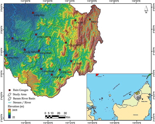
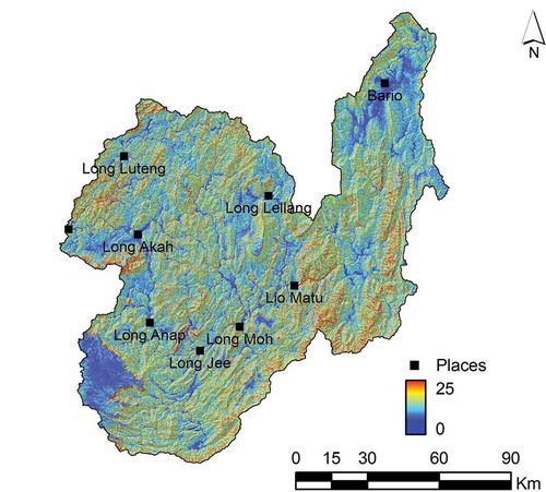
Figure 1. Study area location map with rain gauges

Tropical rainforests regions in Southeast Asia are undergoing rapid depletion due to logging activities and other infrastructure development projects (Lal 1987, Gupta 1996, Achard et al. 2002, Curran et al. 2004, Sidle et al. 2006, Miettinen et al. 2011). In connection with logging activities and other economic development activities, a large quantity of sediment is delivered to the rivers of these regions. Numerous studies have reported increased levels of soil erosion rate and sediment yields from the logged regions in Southeast Asia and Latin America (Lal 1990, Douglas 1996, Nainar et al. 2017). While reviewing the available literature and reports, it was noted that there have been studies dealing with soil erosion issues in Indonesia (Kalimantan region) and certain parts of Malaysia (West Malaysia and Sabah regions) (Besler 1987, Kusumandari and Mitchell 1997, Gregersen et al. 2003, Clarke and Walsh 2006, Halim et al. 2007, Pradhan et al. 2012, Kamaludin et al. 2013, Mojaddadi Rizeei et al. 2016, Roslee 2017), but no detailed studies are reported from the state of Malaysia known as Sarawak, which is undergoing severe terrain alteration in relation to logging activities. Regional studies carried out in Borneo as a whole indicate the extent of logging in Sarawak, especially in the northern and northwestern part. Considering the gap in research data related to soil erosion and sediment yield from Sarawak, the present research was initiated. The study aims to evaluate the spatial and temporal characteristics of soil loss, erosion vulnerability and sediment yield from the upper catchment region of the Baram River at three different time frames over the past 25 years (1991–1994, 2006–2007 and 2015).

2 Study area

Baram River basin, with a total drainage area of 22 000 km², is one of the largest river basins in Sarawak. The river originates from the northern flanks of the central highlands in Borneo, which act as a natural boundary between Malaysia to the north and Indonesia to the south. The area selected for this study is the upper catchment region of the Baram River (8887 km²) (Fig. 1). Geomorphologically and geologically the area is highly complex. The elevation varies between 22 m to 2418 m a.s.l. and the relief features consist of highly undulating hills to high elevated mountains, linear hill ranges and escarpments. The study area shows a variety of typical geomorphological features such as highland plateaus and low-lying flood plains. The geology consists mainly of sedimentary rock formations and very minor basaltic rocks. The major rock types present are sandstone, shale, mudstone, limestone, marlstone, siltstone, conglomerate, slate, phyllite, andesite and dacite basalt of Paleogene to Recent age (Department of Mineral and Geoscience Malaysia 2013). The area is structurally complex, as evidenced by the presence of multi-directional faults and folds which have a direct influence on the drainage networks. The presence of repeated rapids in river beds and varying drainage patterns (parallel, trellis and rectangular) in close spatial proximity with occasional waterfalls is evidence of lithological variations and/or other processes. The main soil types present are residual skeletal (76%) and podzolic (16%) soils derived from shale and sandy shale parent materials (Department of Agriculture 1982a, 1982b). Residual skeletal soils occur mainly on the upper slope and scarp slope positions and podzolic soils in moderately to steeply dissected hills. Both soil types are prone to erosion hazard as classified by the Department of Agriculture (DoA 1982b). The area receives an average annual rainfall greater than 4500 mm, and occasionally annual rainfall even exceeds 6000 mm (Malaysian Meteorological Department 2017). Mean daily temperatures fluctuate between 12 and 38°C. Tropical rainforests (primary and secondary) dominantly cover the area, with a small amount of area given to oil palm plantations and other agricultural practices such as paddy cultivation (both hill paddy and wet paddy) and fruit orchards. Terrain alteration is severe and is related to contouring of hills for oil palm and rubber plantations and to extensive logging activities (Vijith et al. 2018b).

3 Materials and methods

3.1 Assessment of annual soil loss

The analysis of spatial and temporal characteristics of soil erosion rate and its severity was instigated by application of the Revised Universal Soil Loss Equation (RUSLE) in a geographic information system (GIS) environment. The RUSLE is an empirical equation, developed by the US Department of Agriculture (USDA) to quantify the rate of soil erosion from agricultural plots (Wischmeier and Smith 1978) and later modified to its present form by Renard et al. (1991, 1997). This equation gained widespread application in quantifying soil erosion rates and also to determine erosion-vulnerable zones (Millward and Mersey 1999, Lu et al. 2004, Kouli et al. 2009, Prasannakumar et al. 2012, Fernández and Vega 2016, Borrelli et al. 2018). To quantify soil erosion, RUSLE uses meteorological, soil, terrain and land-cover variables as input parameters. The RUSLE can be written as:

(1) $A=R\times K\times LS\times C\times P$(1)

where A is annual soil loss (t ha⁻¹ year⁻¹); R is the rainfall–runoff erosivity factor (MJ mm ha⁻¹ h⁻¹ year⁻¹); K is soil erodibility (t ha h ha⁻¹ MJ mm⁻¹); LS represents the slope length and steepness factors; C is the cover management factor; and P is the conservation practice factor, where LS, C and P are dimensionless. Annual soil loss (A) in the study area was computed by multiplying all the variables in the equation in a raster-based GIS environment.

Information and data required to derive input variables of RUSLE were collected from different sources including government departments and portals serving as open and free sources of information (Table 1). Information collected from government departments includes topographical maps (1:50,000) from the Land Survey Department of Malaysia (JUPEM), soil maps (1:50 000) produced by the Department of Agriculture (DoA) and monthly rainfall data provided by the Department of Irrigation and Drainage (DID), Malaysia. The USGS Earth Explorer website (http://earthexplorer.usgs.gov/) was accessed to download processed elevation surface data from the Shuttle Radar Topographic Mission (SRTM) as well as Landsat images of different time frames. Further, to ensure the quality of the satellite data used, a special request was made to Earth Resources Observation and Science (EROS) Center Science Processing and Architecture (ESPA) to obtain processed datasets. The input variables required to assess the soil erosion rate were derived using ArcGIS 9.3, SAGA 2.1 and ERDAS Imagine 2015 software, and final integration was carried out in the raster processing module of ArcGIS 9.3.

Table 1. Sources, scale and information of data layers used in the study

Data source	Scale/resolution	Variables generated
Topographic sheets (Land Survey Department, Malaysia)	1:50 000	Study area boundary, drainage networks
Soil series maps (Department of Agriculture, Sarawak, Malaysia)	1:50 000	Soil texture and type
Landsat Images (downloaded from USGS Earth Explorer) Landsat 5 Thematic Mapper (TM) (acquired 1991–1994) Landsat 7 Enhanced Thematic Mapper Plus (ETM+) (acquired 2006–2007) Landsat 8 Operational Land Imager (OLI) (acquired on 2015)	30 m × 30 m	NDVI, C factor, land use/land cover, logging roads
SRTM data (downloaded from USGS Earth Explorer) SRTM Version 3–30 m global elevation data (acquired in 2000)	30 m × 30 m	Elevation and LS factor
Rainfall data (monthly between 1990 and 2014) (Department of Irrigation and Drainage, Malaysia)	mm	Rainfall distribution and R factor

It should be noted that in order to assess the temporal variation in annual soil loss, three different time frame datasets were used in the calculation of rainfall–runoff erosivity (R) and cover management (C) factors. The time frames used in the present study are 1991–1994 (T1), 2006–2007 (T2) and 2015 (T3). Selection of time frames to be analysed was made through the rapid assessment of the spatial spread of logging activity in the region. During the 1990s, logging activity was very low and primarily concentrated in the lower reaches; then, since the mid-2000s, due to increased accessibility though the construction of major bridges and greater mechanization of the logging process, most of the study area has undergone severe logging. This continued until 2010 and later, when some areas in the study regions were converted into protected land and no logging was allowed thereafter. Due to the non-availability of cloud-free satellite images to derive the cover management factors, a series of images was used to make a seamless image of the study area corresponding to time frames T1 and T2. In view of this, rainfall data for these periods were taken into account to generate the R factor. Further details on the datasets and the methodology used to derive the individual parameters to assess the spatial and temporal characteristics of soil erosion in the study area are given in the following sections.

3.1.1 Rainfall–runoff erosivity (R) factor

Among the variables of the RUSLE, the effect of erosive rainfall is expressed as the rainfall–runoff erosivity factor, which plays a major role in controlling erosion by initiation of erosion, sediment production, and its delivery and movement from erosion hotspots to downstream (Dabral et al. 2008, Thomas et al. 2018). In similar studies elsewhere, other authors used methods to calculate R factors using high-resolution (minute or hourly) to coarse-resolution (monthly and annual) rainfall data depending on their availability (Morgan 1974, Singh et al. 1981, Fu et al. 2005, Panagos et al. 2015). In the study area there is a lack of minute and hourly records (higher resolution) rainfall data for calculating event-based rainfall erosivity. Therefore in order to calculate the R factor, the available monthly rainfall data from 15 rain gauging stations in and around the study area from the DID was used. Considering the availability of rainfall data and its temporal resolution, the methodology that uses monthly and annual rainfall data for the calculation of R factor was selected in the present study. The R factor calculation methods originally proposed by Wischmeier and Smith (1978) and later modified by Arnoldus (1980) have been widely used in different regions with similar geo-climatic conditions and were applied here (Prasannakumar et al. 2012, Vijith and Dodge-Wan 2018, Vijith et al. 2018a). The rainfall–runoff erosivity equation can be written as:

(2) $\text{R = mathop {mathop sum nolimits{^} }limits\_{12}^{i = 1} 1.735 times {10^{(1.5log 10 left({{{P\_i^2} over P}} right)- 0.08188)}}}$(2)

where the rainfall erosivity, R, is expressed in MJ mm ha⁻¹ h⁻¹ year⁻¹; P_i is monthly rainfall; and P is annual rainfall (both in mm).

In order to calculate the R corresponding to different time frames, monthly rainfall data for the entire 25-year period (1990–2014) was analysed. For time frames T1 and T2, annual rainfall erosivity was derived and mean erosivity was calculated for use in the estimation of annual soil loss. For T3, annual rainfall erosivity of individual stations was used as such in the final calculation (see Appendix Table A1 and Fig 2.(a–c)). Later, using the spatial analyst extension of ArcGIS 9.3, by implementing the inverse distance weighted (IDW) interpolation method, the spatial distribution of rainfall erosivity in the study area was generated during the relevant time frames.

3.1.2 Soil erodibility (K) factor

Soil erosion is heavily dependent on the soil characteristics, e.g. loose unconsolidated soil will erode faster than clayey and sticky soil. There are many factors that control the properties of soil and determine its susceptibility to erosion. These factors vary between soil types and include porosity, permeability, texture, mineralogy (parent rock) and organic matter content (Wischmeier and Smith 1978). Considering the need for generalized and widely applicable soil erodibility factors, Wischmeier and Smith (1978) developed a soil nomograph which considers five measurable properties. These are the percentages of modified silt (0.002–0.1 mm), modified sand (0.1–2 mm), organic matter (OM), soil structure (s) and permeability (p), which have been extensively used to estimate the K factor worldwide. In this study, a soil texture map (1:50 000) produced by the DoA was used to derive the K factor for the Upper Baram catchment. The major soil types present and the area covered by each type are summarized in Table 2. Soil erodibility values corresponding to each type of soil were also collected from the DoA and checked against other studies conducted in Malaysia (Tew 1999, Mir et al. 2010, Ramli and Bahri 2011, Teh 2011, Pradhan et al. 2012). The K factor for each soil texture class was added to the soil textural map, as it is readily available, and then converted into raster format using the assigned K factor values as the population field.

Table 2. Major soil types and proposed soil erodibility values

Soil group	Soil family (local name)	Soil texture	Proposed K factor
Skeletal	Kapit	Residual (saprolite)	0.019
	Meluan	Lithic/paralithic	0.005
	Kapit/Meluan/Tutoh	Residual (clay loam)/lithic/paralithic/colluvium	0.021
	Meluan/Kapit	Lithic/paralithic (residual)	0.005
	Tutoh	Colluvium (clay loam)	0.017
Skeletal – Podzols	Kapit/Silantek	Residual (non-indurated)	0.047
	Bako/Kapit	Sandy loam (residual)	0.010
	Silantek/Kapit	Sandy loam (residual)	0.010
Red-yellow podzolic	Bekenu	Fine loam (residual)	0.007
	Merit	Fine clayey	0.004
	Bekenu/Merit/Nyalau	Fine loamy, fine clayey, coarse loam	0.021
	Merit/Bemang	Fine clay loam	0.017
Andisols	Linau	Clay (residual)	0.009
Peat (oxisols – organic)	Selio/Nibong/Mulu	Residual clay-fine (lateritic with organic content)	0.009
Podzols – arenaceous	Silantek/Tika	Residual (sandy)	0.041
Oxisols	Nibong/Selio	Residual (fine clay)	0.009
Grey-white podzolic – gleysols	Latan/Penara	Clay	0.004
Red-yellow podzolic – arenaceous	Merit/Tika	Fine clayey, sandy	0.038
Organic – gleysols	Bareo/Dalan	Organic, clayey	0.004
Gleysols – alluvial	Bijat/Seduau	Clay (alluvial)	0.009
	Bemang/Dalan	Fine clay loam	0.017
	Julan/Jiwan	Coarse clay loam	0.021
Podzols – organic	Silantek/Umor/Bareo	Sandy loam, residual (organic)	0.010
Organic	Bareo/Umor	Organic (residual)	0.004
Alluvium – red-yellow podzolic	Bemang/Bekenu	Fine loam (alluvial/residual)	0.018
Recent alluvium	Bemang/Seduau	Fine loamy/clayey (alluvium)	0.017

3.1.3 Slope length and steepness (LS) factor

The effect of topography on soil erosion modelling is accounted for by the slope length and steepness (LS) factor. The LS factor describes the combined effect of slope length and steepness (i.e. flow length and its slope gradient) and represents the ratio of soil loss per unit area (Dabral et al. 2008, Terranova et al. 2009, Alexakis et al. 2013). The LS factor has a significant influence over sediment movement from an area, i.e. long, steep slopes deliver more sediment than gentle and shorter slopes (Moore and Burch 1986). In this study, in order to generate the LS factor, a 30-m digital elevation model (DEM) of SRTM data was hydrologically processed to remove any artefacts present in the data. The terrain analysis module of SAGA 2.1.2 (System for Automated Geoscientific Analysis) software was then used to generate the LS factor via the methodology proposed by Moore and Burch (1986), Moore et al. (1991) and Moore and Wilson (1992):

(3) $LS={\left(A_s/22.13\right)}^{0.4}\times {\left(\mathrm{s}\mathrm{i}\mathrm{n}\beta /0.0896\right)}^{1.3}$(3)

where A_s is the specific catchment area. This calculation returned a spatially distributed LS factor map for the entire study area.

3.1.4 Cover management (C) factor

Vegetation can reduce the direct impact of rainfall on the land surface by decreasing its tendency to erode, and this is expressed in the RUSLE by the cover management factor, C. The C factor is attributed to the protection provided by the existing vegetation against erosion, and can be identified by categorizing different land-use/land-cover (LULC) types (Wischmeier and Smith 1978, Zhou et al. 2008). The C factor varies between 1 and 0, indicating a range between no protection and maximum protection against soil erosion. For the calculation of the C factor, different authors use different methods and datasets. Among these methods, the C factor map derived from the normalized difference vegetation index (NDVI) and LULC maps (existing or newly prepared) have gained wide applicability (Karaburun 2010, Zhongming et al. 2010, Durigon et al. 2014, Panagos et al. 2015, Schmidt et al. 2018). In our study, to generate cover management factors at the different time frames studied (T1, T2 and T3), a coupled approach was adopted. For T1 and T2, the NDVI-based cover management factor generation proposed by Van der Knijff et al. (1999, 2000) was used. The proposed methodology uses an exponential function based on the NDVI, the equation for which can be written as:

(4) $C=\mathrm{e}\mathrm{x}\mathrm{p}\left[-\alpha \times \frac{\mathrm{N}\mathrm{D}\mathrm{V}\mathrm{I}}{\left(\beta -\mathrm{N}\mathrm{D}\mathrm{V}\mathrm{I}\right)}\right]$(4)

where α (= 2) and β (= 1) are dimensionless parameters that determine the shape of the curve relating to NDVI, and the C factor is derived through the constant calibration of monthly C factor data.

For T1, Landsat 5 TM satellite images acquired in the period 1991–1994 were used to derive a cloud-free seamless image from which NDVI was established (Fig. 3(a)). Similarly, for T2, Landsat 7 ETM+ (see Table 1) satellite images acquired in the period 2006–2007 were used to generate NDVI (Fig. 3(b)). The reason that NDVI was selected to generate the C factor for T1 and T2 was the non-availability of good images and also the difficulty of producing the supervised classification map (lack of ground truth points and issues in signature collection). Satellite datasets corresponding to T1 and T2 are processed at the USGS EROS ESPA to generate the NDVI data with assured quality to use in spatial analysis. For the same special data, requests (for data on demand) are made to ESPA by selecting the images corresponding to the time frames considered in the analysis. For T3, a LULC map of the study area was generated through supervised classification of Landsat 8 OLI (see Table 1) images for 2015, with extensive field-based validation (Fig. 3(c)). A total of 539 ground truth points corresponding to various land-use types present in the study area were collected by conducting intensive field work during the period 2014–2017. Later, these points were split into two categories, where one set (239 points) was used for signature collection and the other set (300 points) for validation of the supervised classification map, to assess the accuracy. The classification was carried out to estimate the area covered by individual LULC classes present in the study area. Major land-cover classes present in the study area are primary forest, secondary forest, montane forest, mixed agriculture, hill paddy, wet paddy, bushes, shrubs and grasses, water bodies, exposed barren land, pebbles and cobbles in river beds, and artificial surfaces (Vijith et al. 2018b). Areal extents covered by individual LULC types are given in Table 3. The LULC map generated shows an overall accuracy of 82%. For each class of LULC, suitable C factor values were assigned by considering regional studies carried out in soil erosion modelling (Norsahida 2008, Teh 2011, Pradhan et al. 2012, Vijith et al. 2018a).

Table 3. Major land use/land cover (LULC) types and corresponding C factor values assigned to each

LULC type	Area (km^2)	Area (%)	C factor
Primary forest (PFR)	4397.42	49.48	0.003
Secondary forest (SFR)	3413.30	38.41	0.03
Montane forest (MF)	30.46	0.34	0.003
Mixed agriculture (MA)	349.68	3.93	0.60
Hill paddy (HP)	72.42	0.81	0.45
Paddy field (wet) (PF)	5.88	0.07	0.25
Bushes/shrubs/grasses (BSG)	286.81	3.23	0.86
Water body (WB)	29.31	0.33	0
Exposed barren land (EBL)	293.39	3.30	1
Pebbles/cobbles in river bed (PC)	2.59	0.03	0.01
Artificial surface (AS)	5.90	0.07	0.01
Total	8887.17	100%

3.1.5 Conservation practice (P) factor

The conservation practice factor deals with the soil erosion conservation measures introduced along with the land-use practices in an area. Conservation practice (P) factors are specific to individual land uses, and the most common practices are contour tilling, buffer strips, terracing, gully plugging, small check dams, stone bunds and sediment traps (Wischmeier and Smith 1978, Renard et al. 1997, Thomas et al. 2018). Based on type and contribution to the reduction of sediment erosion, the P factor value of each conservation measure will range from 0 (well conserved) to 1 (no conservation practices). In this case, no conservation practices were identified during field surveys.

3.2 Integration of variables to produce the temporal soil loss map

To assess the spatial and temporal characteristics of soil erosion and sediment contributing sources from the upper catchment regions of the Baram River, RUSLE variables corresponding to the three different time frames were integrated using the raster calculator option of the spatial analyst extension of ArcGIS software. The results, expressed as soil loss, erosion vulnerability and the influence of different land-use practices that contribute a higher amount of sediment to erosion, are discussed in detail in the following sections. Further, 500 random points were generated in the study area and the annual soil loss values for each time frame were extracted to compute the statistics. To identify the areas showing increasing and decreasing characteristics for erosion rate and susceptibility, a spatial differencing of soil erosion rate for individual time frames was also carried out.

3.3 Spatial and temporal characteristics of logging roads

Another important development noticed in the study area was the expansion of logging roads that made most of the region accessible. Therefore, an attempt was made to characterize the development of logging roads in the study area at the different time frames considered in the soil erosion assessment. To determine the temporal trend of logging road development, satellite images from 1991, 2001 and 2015 were digitally analysed, logging roads were extracted and their statistics were computed. Finally, a qualitative comparison of logging roads with soil erosion maps for the corresponding time frames was also carried out.

4 Results and discussion

4.1 Spatial and temporal characteristics of RUSLE variables

4.1.1 R factor

The R factor assessed for the different time frames shows varying characteristics (see Table A1). During T1 (1991–1994), the mean annual rainfall in the study area varies between 2096 mm at Bario (the driest station) to 5037 mm at Long Jee (the wettest station). The study area mean was 3700 mm. The R factor estimated for T1 ranges from 1381 MJ mm ha⁻¹ h⁻¹ year⁻¹ (Bario) to 5314 MJ mm ha⁻¹ h⁻¹ year⁻¹ (Long Jee), with a mean of 3666 MJ mm ha⁻¹ h⁻¹ year⁻¹ (Fig. 2(d)). Considering T2 (2006–2007), again Bario had the lowest mean rainfall of 2252 mm and Long Jee showed the highest (5812 mm), with a study area mean of 4120 mm. The R factor calculated for this time frame ranges between 1392 and 5937 MJ mm ha⁻¹ h⁻¹ year⁻¹, being lowest at Bario and highest at Long Jee (Fig. 2(e)). The mean R value for the whole study area was 3733 MJ mm ha⁻¹ h⁻¹ year⁻¹. At T3 (2014), annual rainfall varied from 1796 mm (Bario) to 4470 mm (Long Moh), with a study area mean of 3409 mm, indicating that 2014 was a relatively dry year. The R factor during this time frame ranged between 1788 (Bario) and 5908 (Long Jee) MJ mm ha⁻¹ h⁻¹ year⁻¹, with a mean of 3789 MJ mm ha⁻¹ h⁻¹ year⁻¹ (Fig. 2(f)).

Figure 2. Temporal distribution of: (a–c) rainfall (mm) and (d–f) rainfall erosivity (MJ mm ha⁻¹ h⁻¹ year⁻¹) during the three time frames (T1, T2 and T3). (Places listed are interior villages present in the study area)

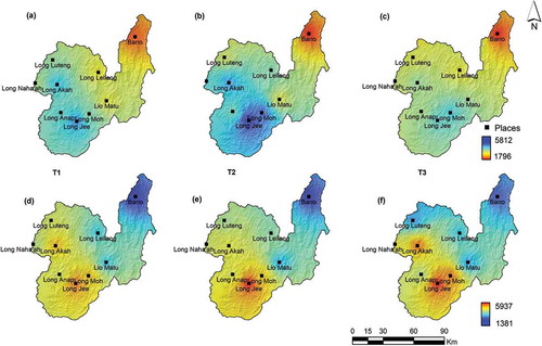
Considering the spatial distribution of rainfall, higher rainfall was found to occur more frequently in the lower reaches of the study area than in the higher elevation places. On the whole, the spatial pattern indicates a similar distribution of rainfall in all time frames, with a higher rainfall corridor in the lower catchment region of the study area. For example, the area around Long Moh, Long Jee and Long Akah showed a comparatively higher amount of rainfall during T2. It was also noted that the upper catchment region, around the areas of Long Lellang, Lio Matu and Bario, shows low mean and annual rainfall totals in all time frames. The R factor also shows a similar spatial pattern, with lower erosivity in the upper catchment (centred on Bario, Lio Matu and Long Lellang) and higher erosivity in the lower catchment, especially around Long Moh, Long Jee and the Long Akah cluster of communities in Baram River corridor.

4.1.2 K factor

There are 26 types of soil in the study area, and these were grouped under 22 textural classes to produce the soil erodibility (K) map. The K factor values vary between 0.004 and 0.047 t ha h ha⁻¹ MJ mm⁻¹ (Table 2 and Fig. 4). The lowest erodibility values are attributed to fine clayey or organic clayey soils, whereas the highest K values are attributed to residual non-indurated soils. Considering the spatial distribution of soil erodibility, most of the study area shows moderate erodibility (K between 0.019 and 0.021 t ha h ha⁻¹ MJ mm⁻¹), with localized areas of higher erodibility.

4.1.3 LS factor

The slope length and steepness (LS) factors, derived from the void-filled DEM, are in the range 0–25 (Fig. 5), with 69% of total study having moderate LS (≤ 7) factor values. The study area has a mean LS of 5. The spatial distribution of LS factor indicates a concentration of higher LS values in steeply sloping hills, escarpments and plateau slopes. It was also noted that a few of the higher elevation places show low LS values, suggesting comparatively smaller terrain undulations in the region. Areas with low LS values are seen around Bario in the upper catchment to the north of the study area, on the Usun Apau Plateau in the southwest and around Long Akah in the southern part of the study area.

4.1.4 C factor

The cover management (C) factor values corresponding to the different time frames show highly varying characteristics. For T1 and T2, the C factor based on NDVI returned a continuous value raster, whereas for T3, an arbitrary value for C was used for each individual LULC mapped through supervised classification, as detailed in Section 3.1.4 (Table 3). The C factors calculated for all three time frames range from 0 (low vulnerability to erosion) to 1 (high vulnerability), with a wide variation in spatial spread of values over the time frames considered (Fig. 3). It should be noted that for the time frame T1, the majority of the study area showed low C values, with higher values concentrated in and isolated to the northern and northwestern parts of the lower catchment region (Fig. 3(d)). For time frame T2, most of the study area showed moderate and higher C factor values (Fig. 3(e)). By time frame T3, the scenario was reversed, with regions of high C factor values appearing more clustered than during the other two time frames (Fig. 3(f)).

Figure 3. Temporal distribution of (a, b) NDVI, (c) land use/land cover and (d–f) corresponding cover management factors. See Table 3 for abbreviations of land-use types

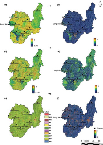
Figure 4. Spatial distribution of K factor in the study area

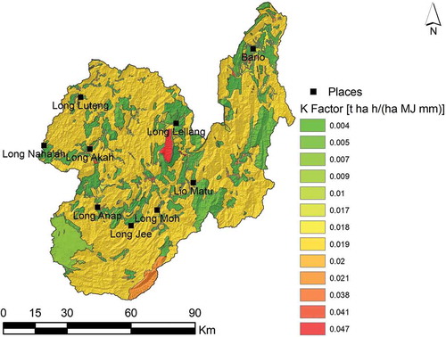
Figure 5. Spatial distribution of LS factor in the study area

The C factor maps generated through two well-established, distinct methods show varying spatial characteristics. This is likely due to the inherent characteristics of the methodology used in this research. The cover management factor maps generated through NDVI-based methods (T1 and T2) show the property of vegetation vigour, which varies in a continuous manner; the values represent a mixed spectral reflectance of material present in each pixel. In contrast, the LULC maps generated through the supervised classification of satellite images show discrete characteristics based on the land-use class attributed to each pixel. Therefore the LULC map can be considered a thematic map which shows non-continuous values. The difference between continuous vs. discrete values has the potential to produce variations in the effect of the cover management factor, C, as observed in our research. A recent study carried out by Vijith et al. (2017) suggests that the LULC-based C factor is suitable for one-time prediction of soil erosion rate if the study ignores the spatial variation in the cover management factor within any land-use type. The area covered by a particular LULC type, e.g. exposed barren land, is assigned a value of 1 for the whole area covered by that class, whereas in the NDVI method, due to minor vegetation variations among the individual pixels, C might be calculated to have a range of values, e.g. ranging from 0.60 to 1. This can result in the observed differences in the spatial pattern of cover management factors generated through two different methods. Considering the overall analytical results and statistical comparison, it can be concluded that both methods have validity in estimating the cover management factor, and both also have limitations. The analysis also indicates that for the assessment of the temporal soil erosion rate, NDVI-based methods are fast and good for generation of the C factor, because they offer the ability to model continuous and progressive variation in cover management factor values, which is more realistic under the given field conditions (Vijith et al. 2017).

The spatial distribution pattern of C factor values over the study period suggests an overall significant increase in vulnerability to erosion between time frames T1 and T2. This can be correlated with the intensification of logging activities between the two time frames. During T1, logging activity was comparatively limited and was concentrated in the lower catchment region. By T2, however, much of the study area was being logged, and erosion vulnerability had increased due to loss of protective cover. So, there was a huge change in vegetation content and terrain characteristics during the period 1990–2000. Considering T3, a well-established pattern of logging can be observed in the region below Bario, which shows more erosion than other places do.

4.2 Spatial and temporal characteristics of soil loss and erosion vulnerability

The RUSLE-based soil losses in each time frame show variations in the total amount of annual soil loss; later, to identify areas of different erosion vulnerability, these were categorized into the three following classes: low (0–5 t ha⁻¹ year⁻¹), moderate (5–25 t ha⁻¹ year⁻¹) and high (>25 t ha⁻¹ year⁻¹). The results for each time frame are discussed in detail below.

4.2.1 Time frame T1 (1991–1994)

In the time frame T1 (Fig. 6(a) and Table 4), soil loss from the study area ranged from 0 to 483 t ha⁻¹ year⁻¹ and showed a highly localized nature, with a mean erosion value for the whole catchment of 2 t ha⁻¹ year⁻¹. Approximately 95% of the area had low erosion vulnerability (Fig. 7(a) and Table 5), while erosion vulnerability was moderate in only 3% of the area and high in less than 2%. In reality, the moderate- and high-vulnerability areas amount to a smaller percentage, as some data anomalies due to minor cloud could not be removed. The higher erosion rates are found to be concentrated in the lower elevation zones of the study area, especially in the Sungai Patah (northern) region, with remaining areas showing relatively low erosion.

Table 4. Maximum and mean erosion rate in different time frames. T1: 1991–1994; T2: 2006–2007; T3: 2015

			Soil loss (t ha^−1 year^−1)
Time frame	Method of C factor calculation	Dataset^a	Maximum	Mean
T1	NDVI	Landsat 5 TM	483	2
T2	NDVI	Landsat 7 ETM+	671	33
T3	Supervised classification	Landsat 8 OLI	1312	27

^aDataset: 30 m × 30 m pixel size.

Table 5. Areal distribution of soil erosion vulnerability classes in the study area in different time frames

	Soil erosion loss range	Time frame 1 (1991–1994)		Time frame 2 (2006–2007)		Time frame 3 (2015)
Soil erosion vulnerability class	(t ha^−1 year^−1)	Area (km^2)	Area (%)	Area (km^2)	Area (%)	Area (km^2)	Area (%)
Low	0–5	8479.21	95.41	3337.46	37.55	5724.06	64.41
Moderate	5–25	253.94	2.86	3646.24	41.03	2160.1	24.31
High	>25	153.85	1.73	1903.30	21.42	1002.84	11.28

4.2.2 Time frame T2 (2006–2007)

In time frame T2, soil loss from the study area varied from 0 to 671 t ha⁻¹ year⁻¹, with comparatively high spatial distribution and showing a considerably small area of relatively low erosion compared to time frame T1 (Fig. 6(b) and Table 4). The mean erosion rate for the entire study area had increased from 2 in T1 to 33 t ha⁻¹ year⁻¹ by T2. Approximately 38% of the area still had low soil erosion vulnerability, indicating a very significant drop from T1 (Fig. 7(b) and Table 5). Around 41% had moderate vulnerability and as much as 21% had high soil erosion vulnerability. This amounts to a 10-fold increase in vulnerable area compared to T1. This is believed to be related to the exposure of the land surface to erosion due to the removal of protective tree cover through logging during the 12 years between T1 and T2. During this time, logging activity was intense and extended into much of the area. These logging areas can be clearly identified from satellite images as exposed barren land, and this was reflected in the estimation of the cover management factor having extreme values (higher vulnerability to erosion).

Figure 6. Spatial distribution of soil erosion rate in different time frames

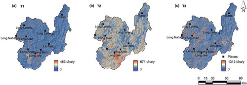
Figure 7. Spatial distribution of soil erosion vulnerability in different time frames

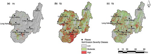
Figure 8. Boxplots explaining the statistical characteristics of soil erosion in the three time frames studied

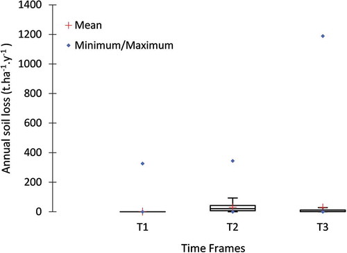
Figure 9. Areal distribution of erosion vulnerability classes in the study area

4.2.3 Time frame T3 (2015)

At T3, the erosion rate ranged from zero to a maximum of 1312 t ha⁻¹ year⁻¹, with co-occurrence of areas having different soil loss rates and a mean erosion rate of 27 t ha⁻¹ year⁻¹ (Fig. 6(c) and Table 4). The spatial pattern shown by the T3 soil erosion rate map indicates more local clustering of high-erosion areas than in the other two time frames. Areas showing relatively high erosion rates are concentrated around Long Luteng, Lio Matu and Long Banga. Classification of the soil loss map according to the soil erosion vulnerability map indicates that low erosion vulnerability zones cover approx. 64% of the area. This is a significant increase in areas under low erosion vulnerability compared with T2 (Fig. 7(c) and Table 5). Twenty-four percent of the area has moderate vulnerability, and the remaining 11% of the area has high soil erosion vulnerability. This is also a significant decrease, i.e. an improvement in comparison to T2.

Annual soil loss estimated at different time frames was extracted through the random points and then used to generate boxplots for better understanding and explanation of the statistical characteristics of annual soil loss at the different time frames (Fig. 8). These data highlight the differences between the time frames in terms of rate of annual soil loss and its distribution in the study area. The boxplots show that although there is a difference in the higher rate of annual soil loss, the distribution characteristics of soil loss for T1 and T3 are similar. Maximum variance was noted in T3, followed by T2, whereas T1 shows the lowest variance in erosion values. At the same time, annual soil loss estimated for T2 shows higher mean and median values than T1 and T3, indicating the occurrence of an almost equal rate of erosion (i.e. high soil loss rate) in the study area during the time frame. Although the T3 samples show a comparatively high rate of erosion, it is noted that the maximum data show a lower rate of erosion (<100 t ha⁻¹ year⁻¹). From the boxplots, it can be inferred that time frame T2 shows a higher rate of erosion than T1 and T3, while there are a few erosion hotspots that deliver a higher rate of sediments during the T3 period. Overall, the study area shows a stabilisation of erosion in T3, but soil erosion hotspots of a very localized nature still exist, which deliver higher amounts of soil during heavy erosive rainfall events.

4.2.4 Comparison with other studies

The results of this research were compared with other soil erosion estimation studies conducted in other parts of Malaysia and Southeast Asia and were found to be similar. For example, Mir et al. (2010) modelled the soil erosion rate from Tasik Chini catchment in West Malaysia by considering different soil series present in the study area; their results show a maximum rate of 348 t ha⁻¹ year⁻¹. Soil loss from the Pahang River Basin in West Malaysia was estimated by Kamaludin et al. (2013), who also identified a relatively high rate of soil loss, of 95.5 t ha⁻¹ year⁻¹. Erosion rates from Penang Island, West Malaysia, estimated by Pradhan et al. (2012), identified a gradual increase in soil loss rate between 2005 and 2010, increasing from 75 to 92 t ha⁻¹ year⁻¹ overall. Also, Mojaddadi Rizeei et al. (2016) identified an increasing trend in soil loss rate from the Semenyih watershed in West Malaysia, with soil losses varying between 43 and 151 t ha⁻¹ year⁻¹ between 2004 and 2010. Soil erosion estimated from the Sabah district of Malaysia shows a severe rate of soil loss exceeding 550 t ha⁻¹ year⁻¹ (Gregersen et al. 2003). Similarly, Russo (2015) attempted to estimate the soil erosion rate from selected cleared areas in Brunei Darussalam and identified severe erosion rates of 1500 t ha⁻¹ year⁻¹. These regions are relatively close to the study area and have undergone similar terrain alteration processes. Detailed studies by the authors (Vijith and Dodge-Wan 2018, Vijith et al. 2018a) in selected sub-basins of the Baram River basin identified severe erosion rates: soil erosion from the Sungai Patah sub-basin of the Baram River basin was estimated at a high rate of 1190 t ha⁻¹ year⁻¹, with a mean loss of 28 t ha⁻¹ year⁻¹. Similarly, the temporal erosion rate estimated for the Sungai Akah sub-basin also showed an increasing trend (mean erosion rates of 4, 6 and 24 t ha⁻¹ year⁻¹ during 1991, 2001 and 2015, respectively) and the maximum rates of soil loss were 1744, 1636 and 1674 t ha⁻¹ year⁻¹, respectively. These results indicate the severity of soil loss from the region, with field and remote sensing observations indicating a connection with logging activities.

Considering the neighbouring countries, soil erosion studies conducted in the Nam Dong and Huong Tra districts of Vietnam by Ham (2008) and Tran et al. (2014) identified an average soil loss of 63.50 and 47.40 t ha⁻¹ year⁻¹, respectively. A recent study conducted by Pham et al. (2018) identified annual soil loss exceeding 50 t ha⁻¹ year⁻¹ from A Sap River Basin in central Vietnam; these authors suggested that the higher erosion rates were contributed by agricultural land and some natural forests. Nontananandh and Changnoi (2012) characterized temporal soil loss from the Songkhram Basin in northeastern Thailand through Internet GIS and USLE. They identified high maximum rates of annual soil losses of 700 and 692 t ha⁻¹ year⁻¹ for 2006 and 2010, respectively, but with comparatively low mean erosion rates (4.94 and 3.95 t ha⁻¹ year⁻¹, respectively).

Studies reported from different provinces of Indonesia also showed comparable high rates of mean soil loss. Saidi et al. (2010) assessed the temporal variation in the soil erosion rate from an agricultural watershed in West Sumatra and identified an increasing trend in mean soil loss rate during the time periods considered. For 1992, the mean annual soil loss was 43.13 t ha⁻¹ year⁻¹; this increased to 58.91 t ha⁻¹ year⁻¹ for 2002. Gusta Gunawan et al. (2013) reported an increase in the mean erosion rate from 3 to 27.30 t ha⁻¹ year⁻¹ within a period of 9 years (2000–2009) from Manjunto Watershed, Bengkulu Province, Indonesia.

From the studies discussed above it is apparent that, overall, most countries in Southeast Asia face severe erosion hazards, with very high values reported from Malaysia and Indonesia.

The spatial distribution of areas with high erosion rates was found to vary significantly between the assessment periods in the study area. Among these, the map corresponding to the period 2006–2007 (T2) suggests a major increase in the spatial spread of high erosion rate areas. Visual inspection of the erosion maps indicates that for the T1 time frame, there was an overall low rate of erosion and limited spatial spread of areas with higher erosion. In comparison, during T2 and ongoing in T3, there are relatively widespread areas characterized by high erosion rates. Output maps of soil loss clearly show a substantial increase in erosion values in the study area between 1990 and 2015, indicating that most of the changes occurred during the period 1994–2006. Moreover, high-elevation zones of the study area (such as the inaccessible Usun Apau Plateau), which are relatively devoid of human activities, can be clearly identified on the maps as they show very low (and sometimes nil) rates of soil loss. Erosion rates estimated during different time frames clearly indicate differential zonation of vegetation disturbances with varying severity in the study area.

4.2.5 Summary

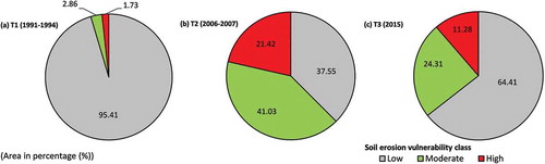
Comparison of three erosion vulnerability maps in terms of area percentage under each class of erosion vulnerability has highlighted that the temporal changes show drastic variations between the time frames considered (Fig. 9). During 1991–1994 (T1), most of the study area could be considered as having low erosion vulnerability. This changed significantly by T2 (2006–2007), as shown by the percentage areas of different vulnerability classes. The percentage of area covered by the low vulnerability zone was reduced from 95% to 38% between T1 and T2 (i.e. within a period of 12 years). Most of the low erosion vulnerability zones became moderate or high vulnerability zones during that time frame. More than 21% of the area became highly vulnerable to erosion. This very significant level of increase, from 2% to 21% in 12 years, indicates the intensification of terrain susceptibility to erosion during this period. This can be attributed to the increased accessibility in the study area and associated intense and widespread logging activity between 1994 and 2006. Maps of soil erosion and regrowth of vegetation in logged forest areas in Borneo indicate that once the terrain in these region loses its natural protection, it will remain an erosion hotspot for a long time and will show high erosion vulnerability. By T3 (2015), most of the region had regained some stability in terms of erosion vulnerability and up to 64% of the area was again characterized by low erosion vulnerability, although more than 11% of the area still had high erosion vulnerability. Considering the results of the soil erosion vulnerability analysis in the three time frames (1991–1994, 2006–2007 and 2015), it can be concluded that the study area still possesses a certain level of high erosion vulnerability, which is directly related to logging and terrain alteration activities in the region.

4.3 Source contributors of sediments in the region

4.3.1 Contribution of LULC

Sources contributing sediments to erosion in the region were identified by comparing the existing land-use map with a recent soil erosion map (T3). Sediment delivery from a region is heavily dependent on a multitude of factors, varying from terrain to meteorological and land-use activities (de Vente et al. 2007, Zhang et al. 2010, Didoné et al. 2015, Noori et al. 2016). The spatial pattern of the soil loss map indicates areas of higher and lower erosion, in which the higher erosion areas are likely to contribute to the sediment delivery if connectivity is efficient (Bracken et al. 2015). In our analysis, during the detailed field mapping and verification of different land-use types (2014–2017), it was observed that several types of land use show spatial variation in their coverage due to various anthropogenic activities in the region. These are strong contributors to soil loss, having high mean annual soil loss. The LULC types that show a higher variation in spatial characteristics are exposed barren land, mixed agriculture, bushes/shrubs and paddy (wet and hill) fields (Vijith et al. 2018b). To assess the sediment contribution from each of these, their respective mean erosion rates were assessed (Table 6). All these LULC classes show comparatively higher ranges of erosion rate with large variation in mean soil loss. It was also noted that, among the identified LULC types, exposed barren land delivers a mean soil loss of 228 t ha⁻¹ year⁻¹ followed by bushes and shrubs (178.76 t ha⁻¹ year⁻¹). The other dynamic land use categories (hill paddy, wet paddy and mixed agriculture) also show comparatively higher rates of sediment removal (141, 98.67 and 88.09 t ha⁻¹ year⁻¹, respectively).

Table 6. Mean soil erosion corresponding to the most dynamic land-use activity in the study area

Land use/land cover	Area (km^2)	Area (%)	Mean soil loss (t ha^−1 year^−1)
Exposed barren land	293.39	3.30	228.00
Mixed agriculture	349.68	3.93	88.09
Bushes/shrubs	286.81	3.23	178.76
Hill paddy	72.42	0.81	141.00
Paddy field	5.88	0.07	98.67

Land-use types that deliver higher amounts of sediment and show higher rates of erosion and vulnerability are the product of human intervention in the region, such as agricultural practices and logging. As an agricultural practice, hill paddy, which is located on steep mountain slopes, had a mean erosion rate of 141 t ha⁻¹ year⁻¹, delivering more sediment per surface area than wet paddy or mixed agriculture. This highlights the influence of LS over the soil loss in these regions. It is thought that this is becasue most hill paddy cultivation is done without any conservation measures, and because forest in the area will continue to be cut and burnt for the purpose. In contrast, mixed agriculture includes small trees and grassland, which are capable of reducing the direct impact of erosive rain, thus reducing the sediment delivery from those areas. In the case of wet paddy cultivation, only over-flooding will cause sediment delivery downstream. However, exposed barren land and bushes/shrubs are both the product of intense logging in the area and major contributors to higher erosion vulnerability, soil loss and sediment yield due to a lack of protective vegetative cover, without which the direct impact of erosive rainfall is severe. Exposed barren land in the study area consists mainly of logging roads and logged areas with tracks. Bushes and shrubs indicate a regeneration of logged areas and are mostly associated with logging roads (sides of hills or on their flanks). Field observations reveal that streams emerging from logged regions are severely turbid due to the increased sediment. It is to be noted that, although exposed barren land and bushes/shrubs only comprise 6.53% of the land use in the total area, these land-use classes contribute more than 49% of total sediment losses. Although the estimates are based on empirical methods, they suggest that over 70% of sediment delivery is from exposed barren land and bushes/shrubs.

4.3.2 Comparison with other studies

These findings were well supported by local and regional studies carried out by other authors in different countries in Southeast Asia that have also undergone severe terrain alteration due to anthropogenic activities – mainly logging. Kasran and Nik (1994) attempted to model suspended sediment yield from a 28.4-ha logged forested catchment in Jengka experimental basin (Malaysia) after different periods of logging. The suspended sediment yield showed a two-fold increase in three consecutive years (yields of 0.10 t ha⁻¹ year⁻¹ in the first year, 0.27 t ha⁻¹ year⁻¹ in the second year and 0.39 t ha⁻¹ year⁻¹ in the third year), while in the fourth year the suspended sediment yield was similar to that in the pre-logged period. A regional-scale comparative study carried out by Gupta (1996) demonstrated the severity of sediment yield from the region due to deforestation and shifting agriculture, urbanization, etc. Considering logged areas, sediment yield was very high (70–150 t ha⁻¹ year⁻¹) during the first 3 years of logging (Lal 1987, Greer et al. 1994). Rijsdijk (2005) characterized land-use-based sediment yield from selected parts of Indonesia. He emphasized that among the land uses, rain-fed agricultural areas, stable trails and unconsolidated trails had maximum sediment yields (of 41, 75 and 433 t ha⁻¹ year⁻¹, respectively). A recent study conducted by Straub et al. (2011) found that the Baram River discharges 2.4 × 10¹⁰ kg year⁻¹ sediment to the South China Sea. It is to be noted that the present study area is the upper Baram River basin, which contributes to that total sediment yield. High sediment discharge and sediment yields from this region are mainly due to logging, skid trails and other terrain alteration in relation to agricultural practices (shifting cultivation, oil palm plantations and rubber plantations).

4.3.3 Contribution of rainfall erosivity

Though the land-use activity in the study region controls the production of sediment by acting as source contributors, the erosivity strength of rainfall determines the detachment, movement and channelization of sediment to downstream parts of the region. In the study area, the region around Bario has the comparatively lowest erosivity potential, whereas areas around Long Jee show higher erosivity in all time frames considered. In the present study, for T1 and T2, average rainfall erosivity was calculated by considering the years of acquisition of satellite images used to generate the C factor. Averaging the R factor for this time frame does not generate any drastic variation in the effect and influence of the R factor over the total soil loss from the region, because in most individual years considered in time frames T1 (1991–1994) and T2 (2006–2007), the rain gauging stations in Bario and Long Jee continued to show the lowest and highest rainfall erosivity, respectively, compared to all other stations in the region.

A recent study of the spatial and statistical trend characteristics of rainfall erosivity in the study area, conducted by the authors (Vijith and Dodge-Wan 2019), also suggests there is a concentration of increased rainfall erosivity in the lower elevation areas along the Baram corridor compared to the higher elevation places in the upper catchment. The results of the soil loss estimated in the present study confirm this, showing higher erosion rates in lower elevation parts of the region. This points towards the combined effect of land-use activities and higher rainfall availability with severe erosion potential in controlling the rate of soil loss from the region. Further, it also indicates that even if the rainfall erosivity is severe, where the area is protected by vegetation, the total amount of soil loss will be much less than in exposed areas.

4.3.4 Spatial distribution of soil loss

Spatial differencing of individual time frames carried out for the soil erosion rate maps gives a very clear picture of the dynamic of soil erosion characteristics of the region in the time frames considered (Fig. 10). Differencing of T1 and T2 shows a widespread increase of erosion covering the vast majority of the study area (Fig. 10(a)). It was also observed that some places showed a reduction whereas others showed a steady rate of erosion. In areas that showed decreasing erosion, it was linear in nature, indicating previously logged regions and existing logging roads. While comparing the erosion rates of T1 and T3, it was noted that although the majority of the study area shows increasing erosion, areas with decreasing erosion rates and no change in erosion are also present and are located throughout the study area (Fig. 10(b)). However, when comparing erosion rates between T2 and T3, a predominantly decreasing erosion rate is observed, and this covers most of the area (Fig. 10(c)). Furthermore, there were isolated and clustered zones with increasing or with no change in erosion rates between these periods. Considering the three spatial differencing maps, it may be concluded that the severity of logging-related effects was greater between T1 and T2 than between T2 and T3.

Figure 10. Spatial distribution of soil loss characteristics of the study area, identified through differencing of erosion rates calculated for the time frames considered

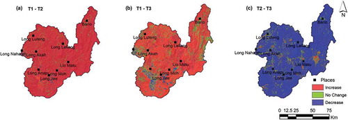
Figure 11. Spatial distribution of logging roads in the different time frames considered

4.4 Spatial and temporal characteristics of logging roads

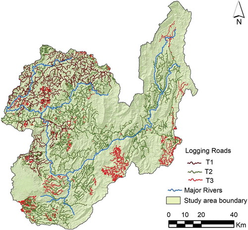
During the analysis, it was noted that zones of severe erosion and higher sediment yields are well correlated with logging activity, especially the development logging roads and skid trails. The spatial pattern of logging roads and their statistics are shown in Fig. 11 and Table 7. In the T1 time frame, logging roads in the study area were concentrated in the lower catchment region, with a total length of 3272 km and a mean density of 0.36 km km⁻². Logging roads showed an increasing trend in the T2 time frame, with a total length of 7539 km, which is a 56% increase over T1. The spatial pattern indicates that the logging road network had extended into the upper catchment and had also extended to both sides of the Baram River. This trend continued in time frame T3, with an increase in the total length of logging roads to 9451 km. As a result of these successive increases, by 2015 (T3), the mean road density had reached 1.06 km km⁻², with a spatial spread across most of the study area. When viewed as a whole from T1 to T3, the development of logging activity in the study area shows roughly a doubling in logging road length and density across each time frame. The trend and spatial spread of logging roads show that their development was strongly influenced by the construction of major bridges across the Baram River, which enabled access to both banks. The Long San bridge in the lower part of the study area allowed access to the right bank, in particular towards Long Banga, and the Long Matapa bridge in the upper part allowed access to the upstream left-bank areas. Both bridges led to intensified logging activity and ultimately contributed to increased soil loss in the study area.

Table 7. Logging road characteristics in the Upper Baram catchment in different time frames. T1: 1991–1994; T2: 2006–2007; T3: 2015

Characteristics analysed	Time frame
	T1	T2	T3
Total length of road networks (km)	3272	7539	9451
Mean density – whole study area (km km^−^2)	0.36	0.84	1.06
Trend (% change^a)	-	+56%	+25%
Logging road clusters^b	Right bank (North)	Right bank (North, northeast)	Left bank (South, southwest)

^aCompared to the previous time frame.

^bCompared with the Baram River basin.

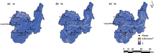
The increase in soil erosion rates observed between the time frames can be explained by the interconnection of soil erosion rate with logging activity and especially the degradation of vegetation associated with the development of logging roads and skid trails. Regions with high density of logging roads and skid trails show a higher rate of soil loss and erosion vulnerability than other areas. Moreover, it was observed that during the first 5 years of the study period, the vast majority (95%) of the study area showed low vulnerability to soil loss and erosion. During that time, the mean road density was 0.36 km km⁻². In the next time frame (T2), the area classified as having low erosion vulnerability had been reduced to 38% and the logging road length and mean density had increased to 7539 km and 0.84 km km⁻², respectively, with a wide spatial spread. By 2015 (T3), 64% of the study area showed low erosion vulnerability, i.e. there was an improvement, but logging road length and mean density, in contrast, had increased further to 9451 km and 1.06 km km⁻², respectively. The increase in low erosion vulnerability areas between T2 and T3 is believed to be related to the stabilization of terrain against erosion after a few years of logging due to regrowth of vegetation. Considering the road density at the spatial scale, it shows variation at the unit scale (Fig. 12). During T1, the road density varied in the range 0–2.57 km km⁻² (Fig. 12(a)), whereas in T2, it had increased to 0–2.91 km km⁻² (Fig. 12(b)). Further, in T3 – as discussed above – the road density had increase to 3.99 km km⁻² (Fig. 12(c)).

Figure 12. Spatial distribution of logging road density in the study area

This increasing road density indicates the severity of logging activity in the region. Our results are well correlated with the findings of Gaveau et al. (2014), who investigated forest clearance and logging in Borneo, and estimated a total length of primary logging roads between 1973 and 2010 of 271 819 km for the whole of Borneo. While considering the different administrative divisions in Borneo, Sarawak (Malaysia) alone was reported to have 82 239 km of logging roads, with a density of 0.89 km km⁻², which is almost double the average density for the entire Island of Borneo (0.48 km km⁻²). This alone highlights the intensity of the logging process in Sarawak as a whole and is supported by our findings in the Upper Baram study area in particular.

5 Summary and conclusion

This study analysed the spatial and temporal characteristics of soil loss, erosion vulnerability and dominant contributors of sediments from severely logged areas in the upper Baram River basin (Sarawak) by applying empirical equations. Three time frames, 1991–1994 (T1), 2006–2007 (T2) and 2015 (T3), were considered in our analysis. Soil loss from the study area varied in the range 0–483 t ha⁻¹ year⁻¹, with a mean of 2 t ha⁻¹ year⁻¹ in time frame T1. For T2, the range and mean are 0–671 and 33 t ha⁻¹ year⁻¹, respectively, and for T3 they are 0–1312 and 27 t ha⁻¹ year⁻¹. Of the three time frames considered, the highest mean erosion rate was that of T2. Soil erosion vulnerability classification indicates a varying trend, with a significantly smaller area (38%) in the low vulnerability class in time frame T2 compared to T1 (95%) and some improvement by T3 (64%). Similarly, highly vulnerable areas also show higher percentage of total area vulnerable to soil erosion in T2 (21%) than in T1 (2%) and in T3 (11%).

Considering the relationship between soil loss and sediment contribution by LULC activities/classes in the region, barren land exposed as a result of logging followed by agricultural activity quantitatively contributed the most to overall soil losses. Logging roads and associated skid trails show a high rate of mean soil loss (228 t ha⁻¹ year⁻¹); in addition, hill paddy cultivation, which covers less than 0.07% of the total area, shows a relatively alarming rate of soil loss (98.67 t ha⁻¹ year⁻¹). Both these contributing factors need to be properly managed to reduce the loss of soil and subsequent reduction of soil fertility in the region. Comparison of the temporal characteristics of logging roads with soil loss and soil loss erosion vulnerability shows a high level of correlation. This was well reflected in the spatial pattern of logging roads and indirectly indicates the extent of logging in the study area during T2 and T3.

In summary, the spatial and temporal variation of soil loss and erosion vulnerability show high dynamicity in relation to the logging activity, and the study finds a 10-fold or greater increase in sediment yield in the upper Baram over the past three decades. The research also demonstrates the acceptability of concurrent use of cover management factors generated through two different methodologies to assess spatial and temporal changes in soil erosion rate and vulnerability. The outcome of this research confirms the need to address and plan proper management strategies specific to land-use activities delivering higher amounts of sediment. Implementation of proper sediment-trapping techniques and channel routing in severely logged areas will reduce sediment delivery and, thus, can reduce overall soil loss and sediment load in major rivers flowing in the region.

Acknowledgements

The authors wish to thank Sarawak Energy Berhad for funding this research under the Project “Mapping of Soil Erosion Risk.” They also thank Curtin University Malaysia for facilities and other assistance and the Department of Irrigation and Drainage (DID), Malaysia, for providing rainfall data. The authors are also thankful to the anonymous reviewers and associate editor Dr. Jesus Rodrigo-Comino for their critical reviews, constructive comments and suggestions, which significantly improved the quality of the manuscript.

Disclosure statement

No potential conflict of interest was reported by the authors.

Additional information

Funding

This research was carried out as part of the project “Mapping of Soil Erosion Risk” funded by Sarawak Energy Berhad (RD01/2014(C)), Malaysia.

Appendix

Table A1. Rainfall (mm) and rainfall–runoff erodibility factor (R, MJ mm/(ha/h year)) corresponding to different time frames. Time frame 1: 1991–1994; time frame 2: 2006–2007; time frame 3: 2015

	Time frame 1										Time frame 2						Time frame 3
	1991		1992		1993		1994		Mean 1991–1994		2006		2007		Mean 2006–2007		2015 (using rainfall of 2014)
Station code	Rainfall	R	Rainfall	R	Rainfall	R	Rainfall	R	Rainfall	R	Rainfall	R	Rainfall	R	Rainfall	R	Rainfall	R
Long Akah	4399	5727	4972	4550	4428	5104	4783	3768	4645	4787	5491	4889	4586	3644	5038	4266	3967	5380
Long Lellang	2986	2651	3050	2857	3499	3428	3180	2569	3179	2876	4307	3391	–	–	4307	3391	3253	2822
Long Naha’ah	4267	4610	3490	3389	3756	3653	3757	3294	3817	3736	4591	4299	4589	3708	4590	4003	3629	4518
Long Luteng	–	–	–	–	–	–	–	–	–	–	3620	3563	3925	3539	3772	3551	3378	2353
Long Anap	3822	3333	4861	4507	4253	3841	4564	4856	4375	4134	4287	3994	4536	4403	4411	4199	3846	3798
Long Jee	4659	6196	5269	4844	5343	5901	4877	4313	5037	5314	5779	5926	5846	5949	5812	5937	4396	5908
Long Moh	4407	5368	3925	4649	4158	4632	3929	4350	4105	4750	5282	4358	5387	4980	5335	4669	4470	5269
Lio Matu	3164	2267	2924	2317	3693	3500	3207	3223	3247	2827	3686	2598	3636	2516	3661	2557	- -	–
Bario	2102	1619	1997	1343	2361	1364	1925	1199	2096	1381	2271	1487	2234	1296	2252	1392	1796	1788
Long Seridan	3463	2902	3055	2623	3149	3111	2150	3043	2954	2920	3779	3000	3904	2872	3842	2936	3342	3207
Pa Tik	–	–	–	–	–	–	–	–	–	–	3730	2762	3502	2540	3616	2651	4136	3357
Long Atip	3685	4495	4409	6582	4157	4767	3075	2622	3831	4616	3636	3232	2359	4625	2998	3928	–	–
Long Pilah	3940	3155	3874	3403	3565	3325	3853	5932	3808	3954	3596	6398	4963	3850	4280	5124	–	–
Long Subing	3282	2510	2881	3514	3220	2373	3793	3226	3294	2906	4011	3634	–	–	4011	3634	2043	3639
Long Aton	3721	3484	3400	3649	3641	3519	4098	3202	3715	3463	4209	5013	3533	2500	3871	3756	2650	3423

References

- Achard, F., et al., 2002. Determination of deforestation rates of the world’s humid tropical forests. Science, 297 (5583), 999–1002. doi:10.1126/science.1070656
- Alexakis, D.D., Hadjimitsis, D.G., and Agapiou, A., 2013. Integrated use of remote sensing, GIS and precipitation data for the assessment of soil erosion rate in the catchment area of Yialias in Cyprus. Atmospheric Research, 131, 108–124. doi:10.1016/j.atmosres.2013.02.013
- Arnoldus, H.M.J., 1980. An Approximation of the rainfall factor in the universal soil loss equation. In: M. De Boodt and D. Gabriels, D, eds. Assessment of erosion. New York: John Wiley and Sons, 127–132.
- Berkun, M., 2010. Hydroelectric potential and environmental effects of multidam hydropower projects in Turkey. Energy for Sustainable Development, 14 (4), 320–329. doi:10.1016/j.esd.2010.09.003
- Besler, H., 1987. Slope properties, slope processes and soil erosion risk in the tropical rain forest of Kalimantan Timur (Indonesian Borneo). Earth Surface Processes and Landforms, 12 (2), 195–204. doi:10.1002/esp.3290120209
- Borrelli, P., et al., 2014. Modeling soil erosion and river sediment yield for an intermountain drainage basin of the Central Apennines, Italy. Catena, 114, 45–58. doi:10.1016/j.catena.2013.10.007
- Borrelli, P., et al., 2018. Object‐oriented soil erosion modelling: A possible paradigm shift from potential to actual risk assessments in agricultural environments. Land Degradation & Development, 29 (4), 1270–1281. doi:10.1002/ldr.2898
- Bracken, L.J., et al., 2015. Sediment connectivity: a framework for understanding sediment transfer at multiple scales. Earth Surface Processes and Landforms, 40 (2), 177–188. doi:10.1002/esp.3635
- Carroll, C., Merton, L., and Burger, P., 2000. Impact of vegetative cover and slope on runoff, erosion, and water quality for field plots on a range of soil and spoil materials on central Queensland coal mines. Soil Research, 38 (2), 313–328. doi:10.1071/SR99052
- Clarke, M.A. and Walsh, R.P.D., 2006. Long-term erosion and surface roughness change of rain-forest terrain following selective logging, Danum Valley, Sabah, Malaysia. Catena, 68 (2–3), 109–123. doi:10.1016/j.catena.2006.04.002
- Curran, L.M., et al., 2004. Lowland forest loss in protected areas of Indonesian Borneo. Science, 303 (5660), 1000–1003. doi:10.1126/science.1091714
- Dabral, P.P., Baithuri, N., and Pandey, A., 2008. Soil erosion assessment in a hilly catchment of North Eastern India using USLE, GIS and remote sensing. Water Resources Management, 22 (12), 1783–1798. doi:10.1007/s11269-008-9253-9
- de Moraes, M.V.A., et al., 2016. Monitoring bank erosion in hydroelectric reservoirs with mobile laser scanning. IEEE Journal of Selected Topics in Applied Earth Observations and Remote Sensing, 9 (12), 5524–5532. doi:10.1109/JSTARS.2016.2574704
- de Vente, J., et al., 2007. The sediment delivery problem revisited. Progress in Physical Geography, 31 (2), 155–178. doi:10.1177/0309133307076485
- de Vente, J. and Poesen, J., 2005. Predicting soil erosion and sediment yield at the basin scale: scale issues and semi-quantitative models. Earth-science Reviews, 71 (1–2), 95–125. doi:10.1016/j.earscirev.2005.02.002
- Department of Agriculture (DoA), 1982a. The soils of northern interior Sarawak (East Malaysia). Malaysia: Department of Agriculture, Sarawak.
- Department of Agriculture (DoA), 1982b. Soil classification in Sarawak. Technical paper no.6. Malaysia: Department of Agriculture, Sarawak.
- Department of Mineral and Geoscience Malaysia (DMGM), 2013. Geological map of Sarawak (1:750,000). Third edition. Malaysia: Directorate of National Mapping.
- Díaz, S., et al., 2006. Biodiversity loss threatens human well-being. PLoS Biology, 4 (8), e277. doi:10.1371/journal.pbio.0040277
- Didoné, E.J., Minella, J.P.G., and Evrard, O., 2017. Measuring and modelling soil erosion and sediment yields in a large cultivated catchment under no-till of Southern Brazil. Soil and Tillage Research, 174, 24–33. doi:10.1016/j.still.2017.05.011
- Didoné, E.J., Minella, J.P.G., and Merten, G.H., 2015. Quantifying soil erosion and sediment yield in a catchment in southern Brazil and implications for land conservation. Journal of Soils and Sediments, 15 (11), 2334–2346. doi:10.1007/s11368-015-1160-0
- Douglas, I., 1996. The impact of land-use changes, especially logging, shifting cultivation, mining and urbanization on sediment yields in humid tropical Southeast Asia: a review with special reference to Borneo. IAHS Publications-Series of Proceedings and Reports-International Association of Hydrological Sciences, 236, 463–472.
- Durigon, V.L., et al., 2014. NDVI time series for monitoring RUSLE cover management factor in a tropical watershed. International Journal of Remote Sensing, 35 (2), 441–453. doi:10.1080/01431161.2013.871081
- Fernández, C. and Vega, J.A., 2016. Evaluation of RUSLE and PESERA models for predicting soil erosion losses in the first year after wildfire in NW Spain. Geoderma, 273, 64–72. doi:10.1016/j.geoderma.2016.03.016
- Fu, B.J., et al., 2005. Assessment of soil erosion at large watershed scale using RUSLE and GIS: a case study in the Loess Plateau of China. Land Degradation & Development, 16 (1), 73–85. doi:10.1002/ldr.646
- García-Ruiz, J.M., et al., 2015. A meta-analysis of soil erosion rates across the world. Geomorphology, 239, 160–173. doi:10.1016/j.geomorph.2015.03.008
- Gaveau, D.L.A., et al., 2014. Four decades of forest persistence, clearance and logging on Borneo. PLoS ONE, 9 (7), e101654. doi:10.1371/journal.pone.0101654
- Greer, T., Bidin, K., and Douglas, I., 1994. Tropical rainforest disturbance and suspended sediment-discharge rating variation. In: L.J. Olive and J.A. Kesby, eds. Variability in stream erosion and sediment tramport: poster contributions (Proc.CanbertdLSymp., December l994). Canberra: Australian Defence Force Academy, Dept. of Geography and Oceanography Special Publ. 5, 34–38.
- Gregersen, B., et al., 2003 January–March. Land use and soil erosion in Tikolod, Sabah, Malaysia. ASEAN Review of Biodiversity and Environmental Conservation (ARBEC), 1–11.
- Gupta, A., 1996. Erosion and sediment yield in Southeast Asia: a regional perspective. IAHS Publications-Series of Proceedings and Reports-International Association of Hydrological Sciences, 236, 215–222.
- Gusta Gunawan, G., et al., 2013. Evaluation of erosion based on GIS and remote sensing for supporting integrated water resources conservation management. (Case study: Manjunto Watershed, Bengkulu Province-Indonesia). International Journal of Technology, 4 (2), 147–156. doi:10.14716/ijtech.v4i2.110
- Halim, R., et al., 2007. Integration of biophysical and socio‐economic factors to assess soil erosion hazard in the Upper Kaligarang Watershed, Indonesia. Land Degradation & Development, 18 (4), 453–469. doi:10.1002/ldr.774
- Ham, H.T., 2008. Soil erosion risk modelling within upland landscapes using remotely sensed data and the RUSLE model (Acase study in Huong Tra district, Thua Thien Hue province, Vietnam). In: International Symposium on Geoinformatics for Spatial Infrastructure Development in Earth and Allied Sciences, 4–6 December. Hanoi, Vietnam.
- Jain, M.K. and Kothyari, U.C., 2000. Estimation of soil erosion and sediment yield using GIS. Hydrological Sciences Journal, 45 (5), 771–786. doi:10.1080/02626660009492376
- Kamaludin, H., et al., 2013. Integration of remote sensing, RUSLE and GIS to model potential soil loss and sediment yield (SY). Hydrology and Earth System Science Discussion, 10 (4), 4567–4596. doi:10.5194/hessd-10-4567-2013
- Karaburun, A., 2010. Estimation of C factor for soil erosion modeling using NDVI in Buyukcekmece watershed. Ozean Journal of Applied Sciences, 3 (1), 77–85.
- Kasran, B. and Nik, A.R., 1994. Suspended sediment yield resulting from selective logging practices in a small watershed in Peninsular Malaysia. Journal of Tropical Forest Science, 7 (2), 286–295.
- Kouli, M., Soupios, P., and Vallianatos, F., 2009. Soil erosion prediction using the revised universal soil loss equation (RUSLE) in a GIS framework, Chania, Northwestern Crete, Greece. Environmental Geology, 57 (3), 483–497. doi:10.1007/s00254-008-1318-9
- Kusumandari, A. and Mitchell, B., 1997. Soil erosion and sediment yield in forest and agroforestry areas in West Java, Indonesia. Journal of Soil and Water Conservation, 52 (5), 376–380.
- Lal, R., 1987. Tropical ecology and physical edaphology. Chichester: Wiley.
- Lal, R., 1990. Soil erosion and land degradation: the global risks. In: Advances in soil science. vol 11. New York, NY: Springer, 129–172.
- Lu, D., et al., 2004. Mapping soil erosion risk in Rondonia, Brazilian Amazonia: using RUSLE, remote sensing and GIS. Land Degradation & Development, 15 (5), 499–512. doi:10.1002/ldr.634
- Malaysian Meteorological Department, 2017. Malaysia’s Climate: seasonal rainfall variation in Sabah and Sarawak. http://www.met.gov.my [Accessed 12 July 2017].
- Martı́nez-Casasnovas, J.A. and Sánchez-Bosch, I., 2000. Impact assessment of changes in land use/conservation practices on soil erosion in the Penedès–Anoia vineyard region (NE Spain). Soil and Tillage Research, 57 (1–2), 101–106. doi:10.1016/S0167-1987(00)00142-2
- Mhangara, P., Kakembo, V., and Lim, K.J., 2012. Soil erosion risk assessment of the Keiskamma catchment, South Africa using GIS and remote sensing. Environmental Earth Sciences, 65 (7), 2087–2102. doi:10.1007/s12665-011-1190-x
- Midmore, D.J., Jansen, H.G., and Dumsday, R.G., 1996. Soil erosion and environmental impact of vegetable production in the Cameron Highlands, Malaysia. Agriculture, Ecosystems & Environment, 60 (1), 29–46. doi:10.1016/S0167-8809(96)01065-1
- Miettinen, J., Shi, C., and Liew, S.C., 2011. Deforestation rates in insular Southeast Asia between 2000 and 2010. Global Change Biology, 17 (7), 2261–2270. doi:10.1111/j.1365-2486.2011.02398.x
- Millward, A.A. and Mersey, J.E., 1999. Adapting the RUSLE to model soil erosion potential in a mountainous tropical watershed. Catena, 38 (2), 109–129. doi:10.1016/S0341-8162(99)00067-3
- Mir, S.I., et al., 2010. Soil loss assessment in the Tasik Chini catchment, Pahang, Malaysia. Geological Society of Malaysia Bulletin, 56, 1–7. doi:10.7186/bgsm56201001
- Mojaddadi Rizeei, H., et al., 2016. Soil erosion prediction based on land cover dynamics at the Semenyih watershed in Malaysia using LTM and USLE models. Geocarto International, 31 (10), 1158–1177. doi:10.1080/10106049.2015.1120354
- Moore, I. and Burch, G. 1986. Sediment transport capacity of sheet and rill flow: application of unit stream power theory. Water Resources Research, 22 (8), 1350–1360. doi:10.1029/WR022i008p01350
- Moore, I.D., Grayson, R.B., and Ladson, A.R., 1991. Digital terrain modelling: A review of hydrological, geomorphological, and biological applications. Hydrological Processes, 5 (1), 3–30. doi:10.1002/hyp.3360050103
- Moore, I.D. and Wilson, J.P., 1992. Length-slope factors for the revised universal soil loss equation: simplified method of estimation. Journal of Soil and Water Conservation, 47, 423–428.
- Morgan, R.P.C., 1974. Estimating regional variations in soil erosion hazard in peninsular Malaysia. Malaysian Nature Journal, 28, 94–106.
- Nainar, A., et al., 2017. Effects of different land-use on suspended sediment dynamics in Sabah (Malaysian Borneo)–a view at the event and annual timescales. Hydrological Research Letters, 11 (1), 79–84. doi:10.3178/hrl.11.79
- Nontananandh, S. and Changnoi, B., 2012. Internet GIS, based on USLE modeling, for assessment of soil erosion in Songkhram Watershed, Northeastern of Thailand. Agriculture and Natural Resources, 46, 272–282.
- Noori, H., Siadatmousavi, S.M., and Mojaradi, B., 2016. Assessment of sediment yield using RS and GIS at two sub-basins of Dez Watershed, Iran. International Soil and Water Conservation Research, 4 (3), 199–206. doi:10.1016/j.iswcr.2016.06.001
- Norsahida, B.S., 2008. Determination of soil erosion parameters for Malaysian conditions using remote sensing and geographic information system approach. Unpublished Master’s Thesis. UniversitiTeknologi Malaysia, 179.
- Panagos, P., et al., 2014. Assessing soil erosion in Europe based on data collected through a European Network. Soil Science and Plant Nutrition, 60 (1), 15–29. doi:10.1080/00380768.2013.835701
- Panagos, P., et al., 2015. Estimating the soil erosion cover-management factor at the European scale. Land Use Policy, 48, 38–50. doi:10.1016/j.landusepol.2015.05.021
- Panagos, P., et al., 2018. Cost of agricultural productivity loss due to soil erosion in the European Union: from direct cost evaluation approaches to the use of macroeconomic models. Land Degradation & Development, 29 (3), 471–484. doi:10.1002/ldr.2879
- Pham, T.G., Degener, J., and Kappas, M., 2018. Integrated universal soil loss equation (USLE) and Geographical Information System (GIS) for soil erosion estimation in A Sap basin: Central Vietnam. International Soil and Water Conservation Research, 6 (2), 99–110. doi:10.1016/j.iswcr.2018.01.001
- Pimentel, D., 2006. Soil erosion: a food and environmental threat. Environment, Development and Sustainability, 8 (1), 119–137.
- Pradhan, B., et al., 2012. Soil erosion assessment and its correlation with landslide events using remote sensing data and GIS: A case study at Penang Island, Malaysia. Environmental Monitoring and Assessment, 184 (2), 715–727. doi:10.1007/s10661-011-1996-8
- Prasannakumar, V., et al., 2012. Estimation of soil erosion risk within a small mountainous sub-watershed in Kerala, India, using Revised Universal Soil Loss Equation (RUSLE) and geo-information technology. Geoscience Frontiers, 3 (2), 209–215. doi:10.1016/j.gsf.2011.11.003
- Ramli, R. and Bahri, I.S.S., 2011. Determination of soil erodiblity, K factor for Sungai Kurau soil series. ESTEEM Academic Journal, 7 (1), 55–65.
- Renard, K.G., et al., 1991. RUSLE: revised universal soil loss equation. Journal of Soil and Water Conservation, 46 (1), 30–33.
- Renard, K.G., et al., 1997. Predicting soil erosion by water: a guide to conservation planning with the Revised Universal Soil Loss Equation (RUSLE). Agriculture Handbook No. 703. Washington, DC: USDA.
- Rijsdijk, A., 2005. Tropical volcanic watershed. Sediment Budgets, 292, 16.
- Roslee, R., 2017. GIS application for comprehensive spatial soil erosion analysis with MUSLE model in Sandakan town area, Sabah, Malaysia. Geological Behavior, 1 (1), 01–05.
- Russo, A., 2015. Applying the revised universal soil loss equation model to land use planning for erosion risk in Brunei Darussalam. Australian Planner, 52 (2), 1–17. doi:10.1080/07293682.2014.957332
- Saidi, A., et al., 2010. Soil erosion characterization in an agricultural watershed in West Sumatra, Indonesia. Tropics, 19 (1), 29–42. doi:10.3759/tropics.19.29
- Schmidt, S., Alewell, C., and Meusburger, K., 2018. Mapping spatio-temporal dynamics of the cover and management factor (C-factor) for grasslands in Switzerland. Remote Sensing of Environment, 211, 89–104. doi:10.1016/j.rse.2018.04.008
- Sidle, R.C., et al., 2006. Erosion processes in steep terrain—truths, myths, and uncertainties related to forest management in Southeast Asia. Forest Ecology and Management, 224 (1), 199–225. doi:10.1016/j.foreco.2005.12.019
- Singh, G., Rambabu, and Subhash, C., 1981. Soil loss prediction research in India. Dehradun: Bull. No. T-12/D-9, CSWCR & TI.
- Southgate, D. and Macke, R., 1989. The downstream benefits of soil conservation in third world hydroelectric watersheds. Land Economics, 65 (1), 38–48. doi:10.2307/3146262
- Straub, M.K., Mohrig, D., and Pirmez, C., 2011. Architecture of an aggradational tributary submarine channel network on the continental slope offshore Brunei Darussalam. In: Application of seismic geomorphology principles to continental slope and base-of-slope systems: case studies from seafloor and near-seafloor analogues. Tulsa, Oklahoma, USA: SEPM Special Publication, 13–30.
- Swarnkar, S., et al., 2018. Assessment of uncertainties in soil erosion and sediment yield estimates at ungauged basins: an application to the Garra River basin, India. Hydrology and Earth System Sciences, 22 (4), 2471–2485. doi:10.5194/hess-22-2471-2018
- Tamene, L., et al., 2017. Mapping soil erosion hotspots and assessing the potential impacts of land management practices in the highlands of Ethiopia. Geomorphology, 292, 153–163. doi:10.1016/j.geomorph.2017.04.038
- Teh, S.H., 2011. Soil erosion modelling using RUSLE and GIS on Cameron highlands, Malaysia for hydropower development. Unpublished Master’s Thesis. University of Iceland, 74
- Terranova, O., et al., 2009. Soil erosion risk scenarios in the Mediterranean environment using RUSLE and GIS: an application model for Calabria (southern Italy). Geomorphology, 112 (3–4), 228–245. doi:10.1016/j.geomorph.2009.06.009
- Tew, K.H., 1999. Production of Malaysian soil erodibility nomograph in relation to soil erosion issues. In: VT soil erosion research and consultancy. Malaysia: Subang Jaya, Malaysia: Tew Kia Hui, 27. ISBN:983-40126-1-6
- Thomas, J., Joseph, S., and Thrivikramji, K.P., 2018. Assessment of soil erosion in a tropical mountain river basin of the southern Western Ghats, India using RUSLE and GIS. Geoscience Frontiers, 9 (3), 893–906. doi:10.1016/j.gsf.2017.05.011
- Tran, T.P., et al., 2014. Modelingsoilerosion within small mountainous watershed in central Vietnam using GIS and SWAT. Journal of Resources and Environment, 4 (3), 139–147.
- Van der Knijff, J.M., Jones, R.J.A., and Montanarella, L., 1999. Soil erosion risk assessment in Italy. European Commission, Directorate General, Joint Research Centre, Space Applications Institute European Soil Bureau. Luxembourg: Office for Official Publications of the European Communities.
- Van der Knijff, J.M., Jones, R.J.A., and Montanarella, L., 2000. Soil erosion risk assessment in Europe. European Commission, European Soil Bureau. Luxembourg: Office for Official Publications of the European Communities.
- van Zelm, R., et al., 2018. Spatially explicit life cycle impact assessment for soil erosion from global crop production. Ecosystem Services, 30, 220–227. doi:10.1016/j.ecoser.2017.08.015
- Vanwalleghem, T., et al., 2017. Impact of historical land use and soil management change on soil erosion and agricultural sustainability during the Anthropocene. Anthropocene, 17, 13–29. doi:10.1016/j.ancene.2017.01.002
- Vijith, H. and Dodge-Wan, D., 2018. Spatio-temporal changes in rate of soil loss and erosion vulnerability of selected region in the tropical forests of Borneo during last three decades. Earth Science Informatics, 11 (2), 171–181. doi:10.1007/s12145-017-0321-7
- Vijith, H. and Dodge-Wan, D., 2019. Spatial and statistical trend characteristics of rainfall erosivity (R) in upper catchment of Baram River, Borneo. Environmental Monitoring and Assessment, 191 (8), 494. doi:10.1007/s10661-019-7604-z
- Vijith, H., Hurmain, A., and Dodge-Wan, D., 2018b. Impacts of land use changes and land cover alteration on soil erosion rates and vulnerability of tropical mountain ranges in Borneo. Remote Sensing Applications: Society and Environment, 12, 57–69. doi:10.1016/j.rsase.2018.09.003
- Vijith, H., Seling, L.W., and Dodge-Wan, D., 2017. Effect of cover management factor in quantification of soil loss: case study of Sungai Akah subwatershed, Baram River basin Sarawak, Malaysia. Geocarto International, 33 (5), 505–521. doi:10.1080/10106049.2016.1273398
- Vijith, H., Seling, L.W., and Dodge-Wan, D., 2018a. Estimation of soil loss and identification of erosion risk zones in a forested region in Sarawak, Malaysia, Northern Borneo. Environment, Development and Sustainability, 20 (3), 1365–1384. doi:10.1007/s10668-017-9946-4
- Walling, D.E. and Webb, B., eds., 1996. Erosion and sediment yield: global and regional perspectives. In: Proceedings of an International Symposium Held at Exeter, UK, from 15 to 19 July 1996 (No. 236). IAHS.
- Wischmeier, W. and Smith, D., 1978. Predicting rainfall erosion losses—A guide to conservation planning. Washington, D.C., USA: U.S. Department of Agriculture Handbook, No. 537.
- Wynants, M., et al., 2018. Pinpointing areas of increased soil erosion risk following land cover change in the Lake Manyara catchment, Tanzania. International Journal of Applied Earth Observation and Geoinformation, 71, 1–8. doi:10.1016/j.jag.2018.05.008
- Zeng, C., et al., 2017. Soil erosion evolution and spatial correlation analysis in a typical karst geomorphology using RUSLE with GIS. Solid Earth, 8 (4), 721. doi:10.5194/se-8-721-2017
- Zhang, X., et al., 2010. Effects of land use change on surface runoff and sediment yield at different watershed scales on the Loess Plateau. International Journal of Sediment Research, 25 (3), 283–293. doi:10.1016/S1001-6279(10)60045-5
- Zhongming, W., et al., 2010. Stratified vegetation cover index: a new way to assess vegetation impact on soil erosion. Catena, 83 (1), 87–93. doi:10.1016/j.catena.2010.07.006
- Zhou, P., et al., 2008. Effect of vegetation cover on soil erosion in a mountainous watershed. Catena, 75 (3), 319–325. doi:10.1016/j.catena.2008.07.010