New neural fuzzy-based machine learning ensemble for enhancing the prediction accuracy of flood susceptibility mapping

ABSTRACT

High-accuracy flood susceptibility maps play a crucial role in flood vulnerability assessment and risk mitigation. This study assesses the potential application of three new ensemble models, which are integrations of the adaptive neuro-fuzzy inference system (ANFIS), analytic hierarchy process (AHP), certainty factor (CF) and weight of evidence (WoE). The experimental area is the Trotuș River basin in Romania. The database for the present research consisted of 12 flood-related factors and 172 flood locations. The quality of the models was evaluated using root mean square error (RMSE) values and the ROC curve (AUC). The results showed that the ANFIS-CF model and the ANFIS-WOE model have a high prediction capacity (accuracy > 91.6%). Therefore, we concluded that ANFIS-CF and ANFIS-WoE are two new tools that should be considered for future studies related to flood susceptibility modelling.

KEYWORDS:

• flood
• ensemble learning
• GIS
• neural fuzzy
• bivariate statistics
• Romania

Editor A. Castellarin Associate editor A. Domeneghetti

1 Introduction

Flood phenomena were responsible for one-third of the economic losses caused by natural disasters, between 1980 and 2016, in the European Union (Kurnik et al. 2017). In terms of the loss of human lives and destruction of property, floods are among the most widespread and severe natural hazards around the world (Adhikari et al. 2010). According to the Centre for Research on the Epidemiology of Disasters (CRED) (Guha-Sapir 2012), in recent decades, the damages and casualties caused by flood phenomena have increased globally. Between 1980 and 2000, the number of causalities related to flood phenomena reached 170 000 (Pelling et al. 2004). In 2011, flood phenomena caused 5202 deaths, being the third most deadly disasters after earthquakes and tsunamis. Worldwide, in 2017 alone, more than 3000 deaths were recorded and more than 50 million people were affected by floods (Below and Wallemacq 2018). Currently, approximately one-third of the global surface, comprising more than 90 countries, is prone to flooding. Overall, floods are more dangerous than other catastrophic natural hazards, such as landslides, earthquakes and volcanoes (Bolt et al. 2013). Alfieri et al. (2018) put the flood frequency on account of socio-economic developments combined with ongoing climate change. Thus, the identification of areas prone to floods is a crucial element for any mitigation strategy towards flood risk (Sarhadi et al. 2012, Tanwattana 2018, Bodoque et al. 2019, Henstra et al. 2019).

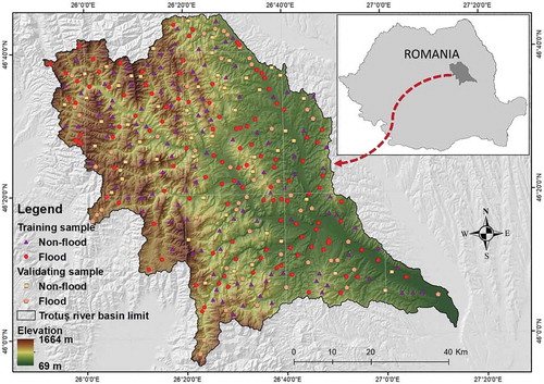
Figure 1. Study area location

Flood susceptibility mapping is an essential activity that is considered the first step in implementing flood risk management and mitigation (Kourgialas and Karatzas 2011). However, according to Dottori et al. (2018), floods are complex processes that are difficult to predict with high accuracy. A review of the literature indicates that various methods have been proposed to identify areas prone to flood hazards. These methods can be separated into four categories: conventional analysis, hydrodynamic simulation, binary pattern recognition and multicriteria-decision making (MCDM) models (Bui Tien and Hoang 2017, Ali et al. 2020). In the first category, frequency and statistical analyses are employed for time-series samples at gauging stations (Petrow and Merz 2009, Lázaro et al. 2016, Yan et al. 2017). Then, regression formulae are constructed to predict discharge dynamics. However, long-term monitoring data are required to produce reliable results.

In the second category, mathematical equations capturing the laws of physics are used to simulate water movements and, finally, to predict flood events (Skaugen et al. 2015, Costa and Fernandes 2017, Masseroni et al. 2017). This category is efficient in flood forecasting, especially when the models are integrated with a geographic information system (GIS) (Skaugen and Onof 2014, El Alfy 2016, Khattak et al. 2016). Additionally, hydrodynamic models can be integrated with both hydraulic and hydrological models to forecast flood risk according to different scenarios. Consequently, various successful models have been proposed, e.g. Hydrologic Engineering Center-River System Analysis (HEC-RAS) (Brunner 1995), HYDROTEL (Fortin et al. 2001), MIKE flood (Zhou et al. 2012) and high-resolution coupled hydrologic-hydraulic model for flash-flood modelling (HiResFlood-UCI) (Nguyen et al. 2016). A detailed review of these hydrodynamic models can be found in (Teng et al. 2017). However, flood processes are typically nonlinear and time-varying, and therefore remain challenging to predict, especially at a regional scale. As reported by Teng et al. (2017), flood modelling is not viable in catchments with areas of more than 1000 km².

For the third category, flood modelling is formulated as a binary pattern recognition problem (Bui Tien and Hoang 2017), in which catchment areas are divided into pixels, which are then classified into flood and non-flood classes. Finally, a decision value belonging to the flood class is used as a flood susceptibility index and, herein, the flood is spatially predicted. Several highly accurate models have been proposed in this category, e.g. frequency ratios (FR) (Tehrany et al. 2014), multivariate statistics (Tehrany et al. 2014), support vector machines (Tehrany et al. 2015, Abedini et al. 2019, Zhao et al. 2019), logistic regression (Nandi et al. 2016), neuro-fuzzy (Bui et al. 2016, Termeh et al. 2018), evidential belief function (Rahmati and Pourghasemi 2017), logistic model trees (Chapi et al. 2017), decision trees (Lee et al. 2017, Khosravi et al. 2018, Yariyan et al. 2020b), multivariate adaptive regression splines (Bui et al. 2019a), weights of evidence (Costache 2019a), genetic algorithm rule-set production (GARP), quick, unbiased and efficient statistical trees (QUEST), random forest (Hosseini et al. 2020), boosted regression trees (Dodangeh et al. 2020) and deep learning neural networks (Bui et al. 2020).

The last category, represented by MCDM methods, includes many algorithms that are based on expert judgement (Costache et al. 2020b, 2020c). Thus, in order to determine the flood susceptibility using MCDM methods, the conditioning factors will be weighted following an expert judgement algorithm. In the last few years, to evaluate flood susceptibility, the following algorithms have been used: analytical hierarchy process (AHP) (Elkhrachy 2015, Costache and Bui 2020), analytical network process (ANP) (Azareh et al. 2019), technique for order preference by similarity to ideal solution (TOPSIS) (Khosravi et al. 2019), simple additive weighting (SAW) (Ameri et al. 2018) and Vlse Kriterijuska Optamizacija i Komoromisno Resenje (VIKOR) (Khosravi et al. 2019).

In recent years, machine learning ensembles have been proposed to improve the prediction quality of flood susceptibility models; these include Bayesian ensemble framework (Costache et al. 2019), hybrid evolutionary algorithms (Bui et al. 2018), swarm-based neural networks (Ngo et al. 2018), ensemble of statistics and machine learning (Choubin et al. 2019, Costache et al. 2020a), decision-making ensemble (Wang et al. 2019a), fuzzy unordered rules induction algorithm (FURIA) ensembles (Bui et al. 2019b), and ensembles of bivariate statistics and artificial intelligence (Costache and Bui 2019, Costache 2019b). Overall, advanced hybrid models are capable of producing promising results (Mosavi et al. 2018, Bui et al. 2020, Talukdar et al. 2020).

In the light of the efficient research trend above, the main goal of the present paper is to expand the body of knowledge of flood modelling by evaluating the potential application of three hybrid models – a neuro-fuzzy inference system (ANFIS) with analytical hierarchy process (AHP), with certainty factor (CF) and with weight of evidence (WoE) – for flood susceptibility mapping. The study will be focused on the Trotuș River basin, which is one of the most flood hazard-exposed areas in Romania.

This research will mainly contribute to enriching our knowledge related to how new machine learning hybrid algorithms can be applied to flood risk management in Romania and other parts of the world. To our knowledge, the present research is the first time the three ensembles, ANFIS-AHP, ANFIS-CF and ANFIS-WOE, have been assessed for use in flood susceptibility modelling.

2 Study area and data used

2.1 General characteristics of the Trotuș River basin

The Trotuş River basin is located in the central–northeastern region of Romania (Fig. 1). The river basin has a slightly oblong shape with a total surface area of 4456 km², and the average slope is 12.5°. The length and the width of the basin are 115 km and 68 km, respectively. This geographical position places the Trotuş River basin in the full temperate zone, where the climatic conditions present a seasonal regime with significant variations in terms of temperature and precipitation. The altitude of the study area varies between 69 and 1664 m a.s.l. The hydrographic network is relatively dense, with average values of 0.3–0.5 km/km² in the hilly area and 0.8–1.2 km/km² in the mountainous area. It is worth noting that the critical surfaces are occupied by floodplains that have slope values close to 0°.

Given the torrential flow conditions in the upper part, as well as the relatively short concentration time within its sub-basins, the study area is exposed to flash floods. These conditions lead, most often, to flooding within the areas at low altitudes, which are also characterized by flat relief. At the catchment level, the mean annual rainfall amount is approximately 800 mm. In 2005, the precipitation recorded between 11 and 13 July represented 100–150% of the multi-annual average for July. It should be mentioned that in 2005 the maximum historical value of the river discharge of 2850 m³/s was recorded (Dumitriu 2019). Thus, flooding is a severe hazard in the Trotuș River basin, strongly affecting areas such as Comănești, Onești, Dărmănești and Târgu Ocna. Moreover, the flood propagating from the upper river catchment towards the lower areas caused serious damage to various sections of national roads: DN11A, DN12A, DN12B, DN2G.

2.2 Historically flooded locations

In the case of studies regarding the identification of areas susceptible to the occurrence of a natural hazard, it is vital to know the physical-geographical properties of the regions where these phenomena occurred in the past (Costache and Bui 2019). For this reason, we consider the identification of historical flood locations within the Trotuș River basin a crucial step in order to achieve a flood susceptibility map that is as accurate as possible. Many data sources were used to extract flood locations, such as governmental sources (Khosravi et al. 2018, Costache 2019b), newspaper articles, field surveys (Nguyen et al. 2017) and remote sensing techniques (Wang et al. 2019b). In order to identify the historical flood locations across the Trotuș River basin, the archive of the General Inspectorate for Emergency Situations of Romania was used. Herein, a total of 172 flood locations was identified and mapped.

2.3 Flood-related factors

Flood genesis is a result of the synergic action of several geographical factors. For this reason, in the case of flood susceptibility studies, it is essential to consider those geographical variables with the highest influence on flood genesis (Costache and Bui 2019). Thus, taking into account the geographical characteristics of the Trotuș River basin and based on the international literature (Costache et al. 2015, Bui et al. 2018, Choubin et al. 2019, Costache 2019c, Pham et al. 2020), in the present study, the following 12 flood conditioning factors were selected: slope angle, topographic position index (TPI), land use, plan curvature (PC), topographic wetness index (TWI), aspect, convergence index, hydrological soil groups, distance from rivers, rainfall, elevation and lithology. The flood predictors represented by slope angle, TWI, TPI, plan curvature, convergence index and elevation were obtained based on the digital elevation model (DEM) at a resolution of 30 m × 30 m. The DEM was extracted from the Shuttle Radar Topography Mission (30 m) database. Land use, lithology and hydrological soil groups were derived from the Corine Land Cover 2018 (Kucsicsa et al. 2019), Geological Soil Map of Romania 1:200 000 (Linzer et al. 1998) and Digital Soil Map of Romania 1:200 000 (Luca and Avram 2017) geodatabases, respectively. A brief description of the flood conditioning factors is presented in the following paragraphs.

Slope angle (Fig. 2(a)) is an important flood conditioning factor because of its direct influence on water accumulation and the surface runoff process (Prăvălie and Costache 2014a, Costache et al. 2015, Zaharia et al. 2015, Tincu et al. 2018, Nhu et al. 2020). Thus, the high slopes determine the flow of water towards the areas with low slopes, which are characterized by a very high potential for water accumulation (Prăvălie and Costache 2013). Slope values are represented in degrees and were separated into the following five classes (Costache 2014a, 2019a, Costache et al. 2020d): 0–3°, 3.1–7°, 7.1–15°, 15.1–25° and 25.1–48.9°. The class of 7.1–15° is encountered on 40.5% of the surface of the research zone and accounts for 5% of the flood locations. Even though the class of 0–3° covers only 10.7% of the study area, more than 68% of the flood pixels are included in this class.

The TPI values (Fig. 2(b)) were divided into the following five classes: −24.4 to −5.1, −5 to −1.4, −1.3 to 1.2, 1.3 to 4.6 and 4.7 to 23.6. The class −1.3 to 1.2 occupies 42% of the study area and overlaps 57.5% of the flood pixels. For land use (Fig. 2(c)), obtained from the CORINE Land Cover 2018 dataset, nine categories were established based on their general characteristics. The nine land-use classes are as follows: built-up areas, agricultural areas, vineyards, fruit trees, pastures, forest, shrub, marsh and rivers. According to the information extracted from the dataset, more than 57.5% of the study area is covered by forests and approximately 17% is covered by agricultural areas. The majority of flood pixels overlap the agricultural areas (35.4%).

Figure 2. Flood predictors: (a) slope angle; (b) topographic position index (TPI); (c) land use; (d) plan curvature; (e) topographic wetness index (TWI); (f) aspect; (g) convergence index (CI); (h) hydrological soil group; (i) distance from rivers; (j) rainfall; (k) elevation; and (l) lithological category

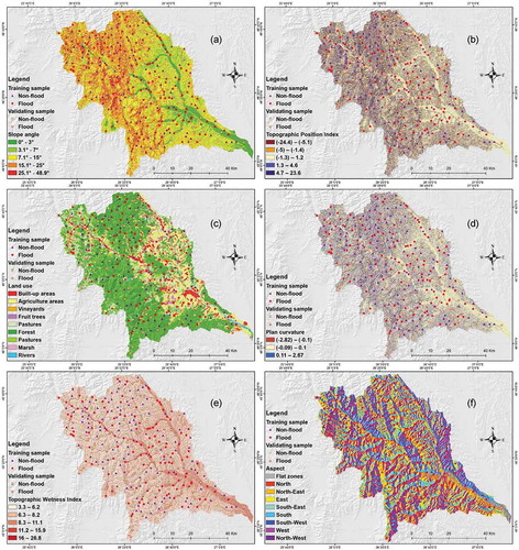
Figure 2. (Continued)

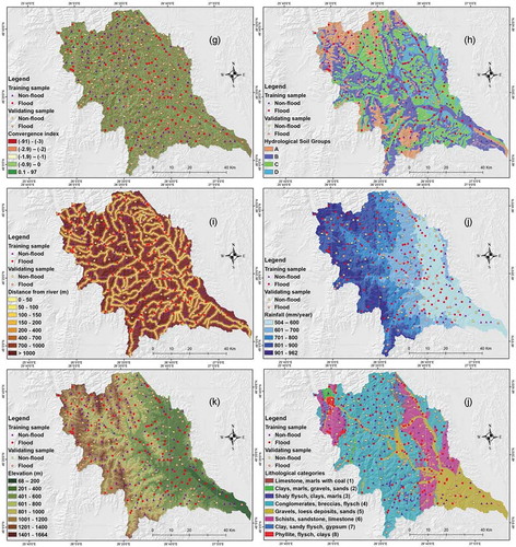
Figure 3. Frequency distribution of flood pixels within the flood predictor classes

TPI - Topographic Position Index; P.C. - Plan curvature; TWI - Topographic Wetness Index; C.I. - Convergence Index; HSG - Hydrological Soil Groups; D.f.R. - Distance from Rivers.

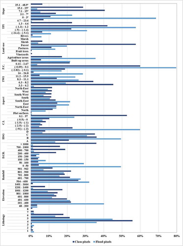
Figure 4. General ANFIS architecture of first-order Takagi-Sugeno fuzzy model

MFs - Membership Functions.

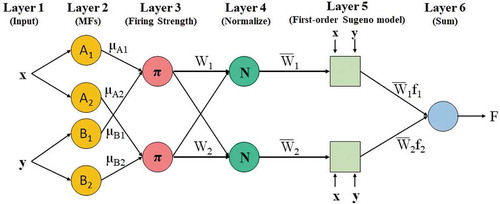
Figure 5. Flowchart of the developed methodology. ANFIS - Adaptive Neuro-Fuzzy Inference System; AHP - Analytical Hierarchy Process; CF - Certainty Factor; WOE - Weights of Evidence; RMSE - Root Mean Sqaured Error; K-index- Kappa Index; FPI - Flood Potential Index

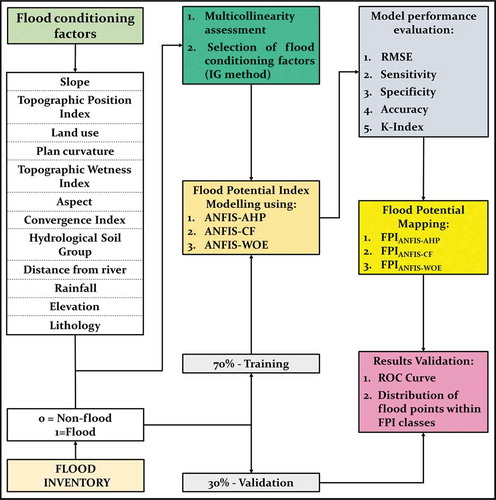
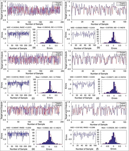
Figure 6. Performance in terms of RMSE calculated for the training dataset: (a) ANFIS-AHP, (c) ANFIS-CF and (e) ANFIS-WOE, and the validation dataset: (b) ANFIS-AHP, (d) ANFIS-CF and (f) ANFIS-WOE

MSE - Mean Squared Error; RMSE - Root Mean Squared Error; StD - Standard Deviation.

The plan curvature (Fig. 2(d)) represents a flood conditioning factor that allows us to detect the areas with a convergent or a divergent runoff phenomenon. This morphometric factor was reclassified into three classes, ranging from −2.82 to 2.67. The class between −0.09 and 0.1 covers 59.9% of the study area and includes 79.6% of the flood pixels.

The TWI is another morphometric flood predictor with a great influence on the flow accumulation process. The values of this index were split into the following five classes: 3.3–6.2, 6.3–8.2, 8.3–11.1, 11.2–15.9 and 16–26.8 (Fig. 2(e)). The class between 3.3 and 6.2 has the largest spatial extent (45.19%) but includes only 1.74% of the flood pixels.

The aspect (Fig. 2(f)) is a flood predictor that has a direct impact on the soil moisture. The eastern slopes cover 14.5% of the area and account for over 20% of the flood pixels, whereas the south-eastern slopes overlap 21.5% of the flood locations.

The convergence index (Fig. 2(g)) is another morphometric flood conditioning factor used in the present study. Its values were divided into five classes taken according to the literature (Zaharia et al. 2017). The class between 0.1 and 97 covers 52.6% of the catchment area and contains 23.8% of the flood pixels. Approximately 59.8% of the flood pixels are located in the class between −91 and −3.

Hydrologic soil groups (Fig. 2(h)) include four soil classes: A, B, C and D (Costache et al. 2014, Costache 2014b, Costache et al. 2020a), each characterized by a different hydraulic conductivity. Group B covers 36% of the area, whereas Group C covers 35%. Approximately 49% of the flood pixels are located within soil Group B, while group C contains 30.8% of the flood locations.

The distance from rivers (Fig. 2(i)) is calculated as the Euclidean distance from a specific point to the closest water course. This factor was reclassified into the following eight classes: 0–50, 50–100, 100–150, 150–200, 200–400, 400–700, 700–1000 and >1000 m. It is notable that the areas within 0 to 100 m of the closest water course cover 8.4% of the catchment’s surface.

Rainfall is a flood predictor that is directly related to the genesis of flood phenomena (Prăvălie and Costache 2014b, Pham et al. 2019). In this research, the rainfall dataset was established using the monitoring values from the weather stations of the National Meteorological Administration of Romania. The spline method was used to interpolate the 23 rainfall values collected from the weather stations. The rainfall values were recorded during the period 1961–2013. The following ranges of values were used to produce the precipitation map: 504–600, 601–700, 701–800, 801–900 and 900–962 mm/year (Fig. 2(j)). The 504–600 mm/year class covers 26% of the Trotuș catchment and overlaps 31.9% of the flood pixels.

Elevation is a morphometric factor that significantly influences the flood potential across a region. It is well known that the water flow drains from the highland areas towards the lowland areas. The following eight classes were delimited for the Trotuș River basin: 68–200, 201–400, 401–600, 601–800, 801–1000, 1001–1200, 1200–1400 and 1401–1664 m a.s.l. (Fig. 2(k)). The 201–400 m elevation class covers 21.9% of the study area and accounts for 40% of the flood pixels. The second class, in terms of percentage of coverage, is the 401–600 m class; it covers 19.7% of the total catchment area. This class accounts for 21.5% of the total flood pixels.

Lithology acts indirectly on the flooding process. Thus, this flood predictor mainly controls the water infiltration process. The lithological characteristics of the area (Fig. 2(l)) were extracted from the geological map of Romania (Linzer et al. 1998) and were reclassified, based on their rock groups, into eight classes. Most of the catchment area is covered by the fourth geological class, representing 55.7%. It should be mentioned that the fourth geological class contains 36% of the flood pixels (Fig. 3). The fifth geological class covers 21.2% of the study area and overlaps 44.7% of the flood pixels.

3 Background on the employed methods

3.1 Adaptive neuro-fuzzy inference system

The ANFIS model is a hybrid between an artificial neural network (ANN) and fuzzy logic (Jang 1993). ANFIS has a self-learning capability without any input conditions. The outputs are provided by the fuzzy logic decisions (Celikyilmaz and Turksen 2009). It is worth noting that the automatic generation of the fuzzy if-then rule, and the parameter optimization of the ANFIS model, can resolve critical problems of the fuzzy system design (Maiti and Tiwari 2014).

The if-then rules are declared as follows:

(1) $Rule1:=\mathrm{i}\mathrm{f}x\mathrm{i}\mathrm{s}{A}_1\mathrm{a}\mathrm{n}\mathrm{d}y\mathrm{i}\mathrm{s}{B}_1,\mathrm{t}\mathrm{h}\mathrm{e}\mathrm{n}{f}_1=p_{1}x+q_{1}y+r_1$(1)

(2) $Rule2:=\mathrm{i}\mathrm{f}x\mathrm{i}\mathrm{s}{A}_2\mathrm{a}\mathrm{n}\mathrm{d}y\mathrm{i}\mathrm{s}{B}_2,\mathrm{t}\mathrm{h}\mathrm{e}\mathrm{n}{f}_2=p_{2}x+q_{2}y+r_2$(2)

where A₁, A₂, B₁ and B₂ represent the membership functions (MFs) for which x and y are the inputs. The consequent parameters are represented by p₁x, q₁yr₁ and r₂ (Jang 1993).

The structure represented by the if-then rules of the ANFIS model corresponds to the Takagi and Sugeno type and holds six layers (Fig. 4). The structure of the layers can be described as follows:

1. The first layer contains the inputs represented by x and y.

2. The second layer consists of adaptive nodes which have the role of creating a degree of membership between the inputs, while the output layers are determined as follows:

(3) $Q_{Ai}={\mu }_{Ai}\left(x\right)fori=1,2$(3)

(4) $Q_{Bj}={\mu }_{Bi}\left(y\right)fori=3,4$(4)

where x and y are the crisp inputs, whereas A_i and B_j are the fuzzy sets (Oh and Pradhan 2011).

• (c) The third layer is made up of fixed nodes (π), which are used as simple multipliers that generate the output. This layer is represented as follows:

(5) $Q_{ij}=W_{ij}={\mu }_{Ai}\left(x\right){\mu }_{Bi}\left(y\right)i,j=1,2,\dots ,n$(5)

where O_ij is the degree to which the previous step was fulfilled.

• (d) The output of the fourth layer is represented through the following relation:

(6) $C_{ij}=\overline{W_{ij}}=\frac{W_{ij}}{W11+W12+W21+W22}i,j=1,2,\dots ,n$(6)

• (e) The fifth layer consists of the adaptive nodes, whose output consists of the product between the normalized values of the third layer and the Sugeno function. The fourth layer is represented as follows:

(7) $T_{ij}=W_{ij}=\overline{W_{ij}}\left(p_{ijx}+q_{ijy}+r_{ij}\right)i,j=1,2,\dots ,n$(7)

• (f) The sixth layer represents the final output of the Adaptive Neuro-Fuzzy Inference Systems model and consists of the sum of the outputs of the fourth layer. The sum is represented as follows:

(8) $\sum \overline{W_{iZj}}=\frac{\sum W_{iZj}}{\sum Zi};i=1,\dots ,n$(8)

3.2 Analytical hierarchy process

The analytical hierarchy process (AHP) method is an algorithm developed by Saaty (1980), which allows any given problem to be solved and analysed in a fast and easy way. The AHP model is very popular in the studies that focus on assessing the degree of susceptibility to natural hazards such as floods. The computational process of the AHP model consists of breaking down a complex problem in a hierarchy with the main objective located at the top level and its criteria and sub-criteria at lower hierarchical levels and sub-levels. The decisional options are located at the lowest part of the hierarchy.

To apply the AHP model for calculating the flood potential index (FPI), the AHP procedure was split into six major steps:

Step 1. Splitting the problem into several components, and setting and defining the objectives.

Step 2. Detailed determination of the criteria and their alternatives.

Step 3. Construction of the pairwise comparison matrix, using the flood-conditioning factors, as well as the pairs formed by their classes or categories. The matrix is constructed based on the influence of each factor class/category in the flood genesis. When a factor has higher importance than another, its relative value will be in the interval between 1 and 9 and is attributed horizontally. In contrast, when a factor is less important than another, its values are assigned vertically and will range from 1/2 to 1/9. Note that the vertical values inside the comparison matrix will be equal to the inverse of those that were assigned horizontally.

Step 4. Use of the eigenvalue algorithm to derive the relative weights for each flood predictor, as well as for each class/category of flood predictors.

Step 5. Computation of the consistency ratio (CR) of the matrix. The CR reflects the quality of the comparison between the pairs. The CR value can be estimated using Equation (10(10) $\mathrm{C}\mathrm{I}=\frac{{\lambda }_{\mathrm{m}\mathrm{a}\mathrm{x}}-n}{n-1}$(10) ), which implies the determination of the consistency index (CI) (Equation (10(10) $\mathrm{C}\mathrm{I}=\frac{{\lambda }_{\mathrm{m}\mathrm{a}\mathrm{x}}-n}{n-1}$(10) )) and the random consistency index (RI). The RI values depend on the number of factors included in the pairwise comparison matrix (Table 1).

(9) $\mathrm{C}\mathrm{R}=\frac{\mathrm{C}\mathrm{I}}{\mathrm{R}\mathrm{I}}$(9)

(10) $\mathrm{C}\mathrm{I}=\frac{{\lambda }_{\mathrm{m}\mathrm{a}\mathrm{x}}-n}{n-1}$(10)

Table 1. Random consistency index (RI; after Saaty 1980)

N	1	2	3	4	5	6	7	8	9	10	11	12	13	14	15
RI	0	0	0.58	0.9	1.12	1.24	1.32	1.41	1.45	1.49	1.51	1.53	1.56	1.57	1.59

where λ represents the highest eigenvalue within the matrix and N is the sum of flood predictors and the number of classes/categories of each factor. The pairwise comparison matrix is indicated by a CR value of less than 0.1.

3.3 Certainty factor (CF)

The CF, developed by Shortliffe and Buchanan (1975), is a bivariate statistical model used to determine the heterogeneity and uncertainty of the input data (Xu et al. 2013). The CF value for each class/category of flood-conditioning factors can be computed using the following equation:

(11) $\mathrm{C}\mathrm{F}=\left\{\begin{array}{c}\frac{\mathrm{P}\mathrm{P}a-\mathrm{P}\mathrm{P}s}{\mathrm{P}\mathrm{P}a\left(1-\mathrm{P}\mathrm{P}s\right)}ifPPa\ge PPs\\ \frac{\mathrm{P}\mathrm{P}a-\mathrm{P}\mathrm{P}s}{\mathrm{P}\mathrm{P}s\left(1-\mathrm{P}\mathrm{P}a\right)}ifPPa<PPs\end{array}\right.$(11)

where PPa is the conditional probability of a flood pixel in class a, whereas PPs presents the prior probability of the total number of flood pixels.

The two above-mentioned probabilities can be calculated as follows:

(12) $\mathrm{P}\mathrm{P}a=\mathrm{P}\left(S/B\right)=\frac{\mathrm{P}\left(S{\cap }^B\right)}{\mathrm{P}\left(B\right)}=\frac{N\mathrm{p}\mathrm{i}\mathrm{x}\left(S{\cap }^B\right)}{N\mathrm{p}\mathrm{i}\mathrm{x}\left(B\right)}$(12)

(13) $\mathrm{P}\mathrm{P}s=\mathrm{P}\left(S\right)=\frac{N_{\mathrm{p}\mathrm{i}\mathrm{x}}\left(\mathrm{f}\mathrm{l}\mathrm{o}\mathrm{o}\mathrm{d}\right)}{N_{\mathrm{p}\mathrm{i}\mathrm{x}}\left(\mathrm{t}\mathrm{o}\mathrm{t}\mathrm{a}\mathrm{l}\right)}$(13)

where P$\left(S/B\right)$ is the conditional probability that unit B contains flood pixels, N_pix(S∩B) represents the sum of the flood pixels in Class B, N_pix(B) represents the sum of the pixels included in Class B, P(S) is the prior probability, N_pix(flood) represents the sum of pixels containing flood locations and N_pix(total) is the sum of the pixels across the entire study area.

3.4 Weight of evidence

Weight of evidence (WoE) is a popular quantitative weighting scheme based on Bayesian statistics (Wod 1985). This method has been successfully used to compute weights in various environmental modelling problems, e.g. landslide, groundwater (Corsini et al. 2009, Regmi et al. 2010) and mineral prospective mapping (Zuo et al. 2015). In this work, WoE was adopted to compute the weights for each class/category of the 12 flood-conditioning factors. Because the WoE model has been well described in the previous literature (Linkov et al. 2009), only the most essential features of this algorithm will be mentioned below.

The first step consists in the computation of the positive weight (W⁺), which indicates the spatial association between the class of a factor and the presence of a flood event:

(14) $W^{+}=ln\frac{\mathrm{P}\left\{B|S\right\}}{\mathrm{P}\{B|\bar{S}\}}$(14)

where W⁺ represents the positive weight, P is the probability rate and B is the presence of flood events, while S and $\bar{S}$ represent the presence and absence of a flood event, respectively.

The next step is the determination of the negative weight (W⁻), which indicates the absence of the spatial association between a predictor and the presence of a flood event (Costache and Zaharia 2017):

(15) $W^{-}=ln\frac{\mathrm{P}\left\{\bar{B}|S\right\}}{\mathrm{P}\{\bar{B}|\bar{S}\}}$(15)

where W⁻ represents the negative weight, P is the probability rate and $\bar{B}$ is the absence of flood events, while S and $\bar{S}$ represent the presence and absence of a flood event, respectively.

Thus, the two equations above could be rewritten as follows (Costache and Bui 2019):

(16) $W^{+}=\mathrm{l}\mathrm{n}\frac{N_{\mathrm{p}\mathrm{i}\mathrm{x}1}/\left(N_{\mathrm{p}\mathrm{i}\mathrm{x}1}+N_{\mathrm{p}\mathrm{i}\mathrm{x}2}\right)}{N_{\mathrm{p}\mathrm{i}\mathrm{x}3}/\left(N_{\mathrm{p}\mathrm{i}\mathrm{x}3}+N_{\mathrm{p}\mathrm{i}\mathrm{x}4}\right)}$(16)

(17) $W^{-}=\mathrm{l}\mathrm{n}\frac{N_{\mathrm{p}\mathrm{i}\mathrm{x}1}/\left(N_{\mathrm{p}\mathrm{i}\mathrm{x}1}+N_{\mathrm{p}\mathrm{i}\mathrm{x}2}\right)}{N_{\mathrm{p}\mathrm{i}\mathrm{x}4}/\left(N_{\mathrm{p}\mathrm{i}\mathrm{x}3}+N_{\mathrm{p}\mathrm{i}\mathrm{x}4}\right)}$(17)

where N_pix1 represents the number of pixels with flood events inside the class, N_pix2 is the number of pixels with flood events outside the class, N_pix3 represents the number of pixels without flood events and N_pix4 is the number of pixels without flood events from outside the class.

Finally, the overall weight of each factor used to compute the FPI was computed using the following mathematical relationship:

(18) $\mathrm{W}\mathrm{f}=W_{\mathrm{p}\mathrm{l}\mathrm{u}\mathrm{s}}+W_{\mathrm{m}\mathrm{i}\mathrm{n}\mathrm{t}\mathrm{o}\mathrm{t}\mathrm{a}\mathrm{l}}-W_{\mathrm{m}\mathrm{i}\mathrm{n}}$(18)

where W_plus represents the positive weight of a flood-conditioning factor, W_mintotal is the total of all negative weights and W_min is the negative weight.

4 Proposed new ensemble methods for predicting the flood-susceptible area

In this paper, the flood susceptibility will be estimated using three hybrid models generated by the combination of the ANFIS algorithm on the one hand with, respectively, the AHP, CF and WOE method on the other hand. The workflow developed in this regard is described below and schematically represented in Fig. 5.

4.1 Establishment of the Trotuș River catchment database

The first step is the establishment of a database that will be used to train the models for flood susceptibility assessment. The database includes 12 flood predictors and 172 flood locations. In this research, flood modelling is formulated as binary pattern recognition (Bui et al. 2016); therefore, 172 non-flood locations were sampled using ArcGIS 10.5 software and included in the database.

4.2 Preparation of the training dataset and the validation dataset

The second step was the preparation of the training dataset and the validation dataset. Taking into account the previous studies (Costache and Zaharia 2017, Moradi et al. 2019, Wang et al. 2019b, Avand et al. 2020, Yariyan et al. 2020a), in order to train the models, the flood predictors were used along with 70% of the flood and non-flood locations. The other 30% of the flood and non-flood locations were used for confirming the model. In this regard, with the help of the “Subset feature” tool in ArcGIS 10.5, the flood and non-flood points were split into training and validating datasets. Thus, 120 flood locations and 120 non-flood locations were included in the training sample, while 52 flood and non-flood locations each were assigned to the validation sample. Note that the flood points were encoded as ‘1’ while the non-flood locations were encoded as ‘0’.

4.3 Multicollinearity check and selection of flood conditioning factor

Another critical step in this workflow is the check for multicollinearity and the selection of flood predictors based on their predictive ability. The multicollinearity check is intended to reduce the redundant information between the flood predictors (Costache 2019b). In contrast, the flood conditioning selection process is applied to remove any information that is irrelevant for flood susceptibility assessment (Costache and Bui 2019). Thus, the variance inflation (VIF) and tolerance (TOL) indicators, computed using SPSS 23 software, are used to estimate the multicollinearity between the flood predictors, while the information gain (IG) method, implemented in Weka 9.2 software, is employed for flood conditioning selection.

4.4 Establishing and training ensemble models

In this fourth step, the proposed hybrid models used in this study were produced by combining ANFIS with (individually) AHP, CF and WoE. Thus, the configuration of the three hybrid models required, in the first stage, the calculation of AHP, CF and WOE coefficients for each factor class/category. These values were determined by applying the methodology described in sections 3.2, 3.3 and 3.4. Note that all values of the three types of coefficients were normalized between 0.1 and 0.9 as follows (Costache and Bui 2019):

(19) $y=\frac{\left(x-min\left(d\right)\right)\times \left(max\left(n\right)-\mathrm{m}\mathrm{i}n\left(n\right)\right)}{max\left(d\right)-\mathrm{m}\mathrm{i}\mathrm{n}\left(d\right)}+\mathrm{m}\mathrm{i}\mathrm{n}\left(n\right)$(19)

where y is the standardized value of x, x is the current value of the variable, d represents the range value limits, and n represents the standardization range limits.

Thus, AHP, CF and WOE have a role of coding flood-related factors for the ANFIS ensemble models (ANFIS-AHP, ANFIS-CF and ANFIS-WOE). Thus, the coding process was performed using a script developed by us in MATLAB software. For each of the three ensembles, the root mean square error (RMSE) was also determined in the case of both training and validating samples. It should be noted that the RMSE parameter was used on a large scale in the previous studies that evaluate the susceptibility of natural hazards with the help of classification applied via the ANFIS model (Hong et al. 2018, Termeh et al. 2018, Tien Bui et al. 2018, Ahmadlou et al. 2019). In this study, the reliability of the model is also tested using several classification metrics, such as sensitivity, specificity, accuracy and k index.

4.5 Generating flood susceptibility maps

In Step 5, flood susceptibility maps were created by multiplying the weights of the flood predictors determined through the ANFIS-AHP, ANFIS-CF and ANFIS-WOE models with the values of the coefficients for AHP, CF and WOE. These operations were performed in ArcGIS 10.5 software.

4.6 Validation of results (ROC curve and density of flood pixels within FPI classes)

Finally, the performance of the flood models was checked using the receiver operating characteristic (ROC) curve and density of flood pixels within the FPI classes. The ROC curve is a graphic in which the x-axis represents the specificity, while the y-axis represents the sensitivity. Specificity refers to the number of incorrectly classified flood locations based on the total number of predicted non-flood locations, while the sensitivity is the number of correctly classified flood locations relative to the total number of flood locations. The area under the curve (AUC) can be derived using the following relationship:

(20) $\mathrm{A}\mathrm{U}\mathrm{C}=\frac{\left(\sum \mathrm{T}\mathrm{P}+\sum \mathrm{T}\mathrm{N}\right)}{\left(P+N\right)}$(20)

where TP (true positive) is the sum of flood pixels correctly classified as floods, TN (true negative) is the sum of non-flood pixels classified as non-floods, P is the sum of flood pixels and N is the sum of non-flood pixels.

The closer the AUC value is to 1, the more efficient the model is. The density of flood locations within the classes of FPI was the second method used in the present study to evaluate the performance of the applied models. The higher the density of flood locations within the high and very high classes of FPI, the better are the applied models.

5 Results

5.1 Multicollinearity assessment and selection of flood conditioning factors

As mentioned in Section 4.3, the multicollinearity assessment was based on the VIF and TOL values. The values of VIF varied between 1.04 (hydrological soil group) and 1.21 (slope angle), while the TOL values range from 0.83 (plan curvature) to 0.96 (aspect). Based on these values, it can be concluded that no serious multicollinearity is present among the flood predictors. The IG values revealed that the highest predictive ability was established for slope angle (0.85), followed by distance from river (0.71), land use (0.67), lithology (0.53), elevation (0.48), plan curvature (0.46), TWI (0.41), TPI (0.39), convergence index (0.37), hydrological soil group (0.32), rainfall (0.29) and aspect (0.18) (Table 2). Given that all IG values are greater than 0, we can accept that all the flood influencing variables have a specific influence on the flooding process. Therefore, all variables will be considered in the analysis.

Table 2. Multicollinearity analysis and predictive ability of independent variables. TPI: topographic position index; TWI: topographic wetness index; TOL: tolerance; VIF: variance inflation; IG: information gain

Flood predictor	TOL	VIF	IG
Slope angle	0.89	1.21	0.85
TPI	0.91	1.12	0.39
Land use	0.85	1.16	0.67
Plan curvature	0.83	1.12	0.46
TWI	0.84	1.09	0.41
Aspect	0.96	1.14	0.18
Convergence index	0.86	1.16	0.37
Hydrological soil groups	0.91	1.04	0.32
Distance from rivers	0.94	1.08	0.71
Rainfall	0.88	1.19	0.29
Elevation	0.85	1.11	0.48
Lithology	0.95	1.04	0.53

5.2 ANFIS-AHP ensemble

The first step to calculate the flood susceptibility through the ANFIS-AHP hybrid model was the computation of the weight of each factor class/category through the AHP multicriteria decision making model. These coefficients resulted from the application of all the pairwise comparisons between the classes/categories of the same factor. Thus, 12 pairwise comparison matrices resulted, and these are included in Table 3. It should be mentioned that the achievement of these matrices was based on expert judgement. The highest weights were assigned to the classes/categories of factors that enhance the probability of flood phenomena, such as slope angles between 0 and 3° (0.516), TPI values between −24.4 and −5.1 (0.416), built-up areas (0.268) and negative values of CI. Further, all the values were normalized in the range 0.1 to 0.9. It should be noted that the CR was also determined to evaluate the consistency of judgement for each of the 12 matrices (Table 4). These values ranged from 0.002 for elevation to 0.064 for curvature plan. Given that all values were below 0.1, it can be stated that all comparisons are consistent.

Table 3. Pairwise comparison matrices

	Pairwise comparison matrix
Factor class/category	[1]	[2]	[3]	[4]	[5]	[6]	[7]	[8]	[9]	Weight	Normalized weight
Slope angle (°)
[1] 0–3	1									0.516	0.90
[2] 3.1 to 7	1/3	1								0.257	0.47
[3] 7.1 to 15	1/5	1/3	1							0.119	0.23
[4] 15.1 to 25	1/7	1/4	1/2	1						0.068	0.15
[5] 25.1 to 48.9	1/9	1/7	1/4	1/2	1					0.039	0.10
TPI
[1] −24.4 to −5.1	1									0.416	0.90
[2] −5 to −1.4	1/2	1								0.262	0.55
[3] −1.3 to 1.2	1/3	1/2	1							0.161	0.32
[4] 1.3 to 4.6	1/4	1/3	1/2	1						0.099	0.18
[5] 4.7 to 23.6	1/5	1/4	1/3	1/2	1					0.062	0.10
Land use
[1] Built-up area	1									0.268	0.90
[2] Agriculture area	1/3	1								0.108	0.37
[3] Vineyard	1/4	1/2	1							0.065	0.23
[4] Fruit trees	1/4	1/2	1	1						0.068	0.24
[5] Pasture	1/2	2	3	2	1					0.198	0.67
[6] Forest	1/7	1/4	1/3	1/4	1/5	1				0.026	0.10
[7] Shrub	1/4	1/2	1	2	1/3	3	1			0.072	0.25
[8] Marsh	1/4	1/2	1	1	1/4	3	1	1		0.063	0.22
[9] River	1/2	2	2	2	1/3	5	2	2	1	0.131	0.45
Plan curvature
[1] −2.82 to −0.1	1									0.175	0.10
[2] −0.09 to 0.1	4/3	1								0.303	0.40
[3] 0.11 to 2.67	4	4/3	1							0.521	0.90
TWI
[1] 3.3 to 6.2	1									0.428	0.90
[2] 6.3 to 8.2	1/2	1								0.259	0.55
[3] 8.3 to 11.1	1/3	2/3	1							0.187	0.40
[4] 11.2 to 15.9	1/5	1/4	1/3	1						0.084	0.19
[5] 16 to 26.8	1/7	1/6	1/5	1/3	1					0.042	0.10
Aspect
[1] Flat surfaces	1									0.032	0.10
[2] North	4	1								0.074	0.28
[3] Northeast	5	2	1							0.109	0.44
[4] East	5	3	4	1						0.216	0.90
[5] Southeast	4	4	2	3/4	1					0.169	0.70
[6] South	4	3/2	3/2	2/3	2/3	1				0.137	0.56
[7] Southwest	3	4/3	1	2/3	3/4	4/5	1			0.114	0.46
[8] West	3	5/4	2/3	2/5	2/5	3/5	4/5	1		0.087	0.34
[9] Northeast	2	1	1/2	1/3	1/2	1/3	3/7	3/4	1	0.062	0.23
Convergence index
[1] −91 to −3	1									0.431	0.90
[2] −2.9 to −2	1/2	1								0.253	0.53
[3] −1.9 to −1	1/3	1/2	1							0.182	0.39
[4] −0.9 to 0	1/5	1/3	1/3	1						0.090	0.19
[5] 0.1 to 97	1/7	1/5	1/5	1/3	1					0.044	0.10
Hydrological soil group
[1] A	1									0.108	0.10
[2] B	4/3	1								0.157	0.19
[3] C	2	4/3	1							0.201	0.27
[4] D	5	3	3	1						0.534	0.90
Distance from rivers (m)
[1] 0–50	1									0.321	0.90
[2] 50–100	1/2	1								0.220	0.63
[3] 100–150	1/3	1/2	1							0.151	0.45
[4] 150–200	1/4	1/3	1/2	1						0.103	0.32
[5] 200–400	1/5	1/4	1/3	1/2	1					0.082	0.26
[6] 400–700	1/6	1/5	1/4	1/3	1/3	1				0.062	0.21
[7] 700–1000	1/7	1/6	1/5	1/4	1/4	1/4	1			0.041	0.16
[8] >1000	1/9	1/7	1/6	1/5	1/5	1/6	1/7	1		0.020	0.10
Rainfall (mm/year)
[1] 504–600	1									0.046	0.10
[2] 601–700	2	1								0.075	0.15
[3] 701–800	4	3	1							0.157	0.31
[4] 801–900	6	4	2	1						0.247	0.48
[5] 901–962	7	5	4	3	1					0.475	0.90
Elevation (m)
[1] 68–200	1									0.318	0.90
[2] 201–400	1/2	1								0.217	0.63
[3] 401–600	1/3	1/2	1							0.151	0.45
[4] 601–800	1/4	1/3	1/2	1						0.132	0.40
[5] 801–1000	1/5	1/4	1/3	1/3	1					0.078	0.26
[6] 1001–1200	1/6	1/5	1/4	1/5	1/3	1				0.049	0.18
[7] 1201–1400	1/7	1/6	1/5	1/6	1/4	1/2	1			0.033	0.14
[8] 1401–1664	1/9	1/7	1/7	1/7	1/5	1/5	1/3	1		0.020	0.10
Lithology
[1] 1	1									0.061	0.20
[2] 2	3	1								0.120	0.38
[3] 3	2	2	1							0.135	0.42
[4] 4	2	1	1	1						0.128	0.40
[5] 5	1/3	1/4	1/4	1/5	1					0.026	0.10
[6] 6	2	1	1	1/2	5	1				0.113	0.36
[7] 7	1	1/2	1/2	1	3	1/2	1			0.123	0.39
[8] 8	7	3	3	2	9	5	1/2	1		0.294	0.90

Table 4. Pairwise comparison matrix properties. CI: consistency index; CR: consistency ratio; RI: random consistency index; TPI: topographic position index; TWI: topographic wetness index

Factor	N	λmax	CI	RI	CR
Slope angle	5	5.114	0.028	1.12	0.025
TPI	5	5.068	0.017	1.12	0.015
Land use	9	9.269	0.034	1.45	0.023
Plan curvature	3	3.074	0.037	0.58	0.064
TWI	5	5.120	0.030	1.12	0.027
Aspect	9	9.256	0.032	1.45	0.022
Convergence index	5	5.140	0.035	1.12	0.031
Hydrological soil group	4	4.011	0.004	0.90	0.004
Distance from rivers	8	8.255	0.036	1.41	0.026
Rainfall	5	5.158	0.040	1.12	0.035
Elevation	8	8.018	0.003	1.41	0.002
Lithology	8	8.119	0.017	1.41	0.012

Normalized values, along with flood and non-flood locations, were used to train the ANFIS-AHP model. RMSE values were used to evaluate the degree to which the targets match the outputs (Fig. 6). In the case of the ANFIS-AHP model, the RMSE was 0.2072 for the training dataset and 0.2434 for the validation dataset. Therefore, we can state that the ANFIS-AHP model has a high accuracy for both training data and validation data.

To emphasize the quality of the models applied in the present research, several metrics such as sensitivity, specificity, accuracy and k index were computed for all flood models (see section 5.3). For the ANFIS-AHP model, the training dataset revealed sensitivity, specificity, accuracy and k values of 0.909, 0.916, 0.913 and 0.825, respectively. The corresponding values for the validation dataset were 0.882, 0.868, 0.875 and 0.808. These parameters indicate that the performance of the model is very good.

Another important result offered by the ANFIS-AHP model in this analysis is the values of the relative importance of the flood conditioning factors. The highest weights resulted for the slope angle (13.97%), followed by distance from rivers (13.65%), land use (12.06%), TWI (10.79%), convergence index (9.21%), lithology (7.62%), rainfall (7.3%), elevation (7.3%), plan curvature (6.9%), TPI (6.67%), hydrological soil groups (6.35%) and aspect (5.08%) (Fig. 7).

The weights of the 12 factors were used to determine the FPI using the ANFIS-AHP hybrid model. Thus, the FPI_ANFIS-AHP values between 0.22 and 0.81 were grouped into five classes, using the natural breaks method. The first class of values, between 0.22 and 0.34, appears on about 21.14% of the whole Trotuș River basin (Fig. 8). The second class, which designates the low values of FPI_ANFIS-AHP, occupies the largest areas, being distributed on about 35.57% of the study area. The average values of FPI_ANFIS-AHP, between 0.41 and 0.45, covered a quarter of the study area (24.69%), while the high and very high values are found in 18.6% of the total area. High and very high susceptibility to floods characterize the areas within the closest proximity to and along the main rivers in the catchment.

5.3 ANFIS-CF ensemble

Table 5 shows the CF values for all classes/categories of flood factors in this research. Table 5 shows that the highest CF value (0.94) is for the 16.0–26.8 class of TWI, followed by the 0–50 m class of distance from river, and then the “rivers” land-use category. Subsequently, these CF values were coded by normalizing all values in the range between 0.1–0.9 for the ANFIS model (Table 5).

Table 5. Certainty factor (CF) and weight-of-evidence (WOE) coefficients. TPI: topographic position index; TWI: topographic wetness index

Factors	Class	Class pixels	Flood	CF	WOE	CFN	WOEN
Slope angle (°)	0 to 3	534565	79	0.84	2.51	0.90	0.90
	3.1 to 7	680406	26	0.37	0.29	0.70	0.55
	7.1 to 15	2007111	10	−0.79	−2.28	0.19	0.14
	15.1 to 25	1421526	5	−0.85	−2.49	0.16	0.10
	25.1 to 48.9	312256	0	−1.00	−2.50	0.10	0.10
TPI	−24.4 to −5.1	309626	14	0.46	0.56	0.90	0.90
	−5 to −1.4	1098837	37	0.28	0.32	0.79	0.85
	−1.3 to 1.2	2082632	66	0.24	0.39	0.77	0.86
	1.3 to 4.6	1117893	2	−0.93	−2.97	0.10	0.10
	4.7 to 23.6	346876	1	−0.88	−2.32	0.13	0.25
Land use	Built-up area	277617	26	0.74	1.71	0.84	0.76
	Agriculture area	845085	39	0.48	1.03	0.73	0.62
	Vineyard	33450	0	−1.00	−1.55	0.10	0.10
	Fruit trees	22613	0	−1.00	−1.55	0.10	0.10
	Pasture	562104	16	0.15	0.36	0.59	0.49
	Forest	2851025	24	−0.65	−1.51	0.25	0.11
	Shrub	313819	5	−0.34	−0.27	0.38	0.36
	Marsh	2149	0	−1.00	−1.55	0.10	0.10
	River	47993	10	0.88	2.40	0.90	0.90
Plan curvature	−2.82 to −0.1	928127	21	−0.07	−0.43	0.66	0.59
	−0.09 to 0.1	2971217	92	0.22	0.44	0.90	0.90
	0.11 to 2.67	1056520	7	−0.73	−1.82	0.10	0.10
TWI	3.3 to 6.2	2239313	2	−0.96	−3.80	0.10	0.10
	6.3 to 8.2	1699284	23	−0.44	−0.70	0.32	0.45
	8.3 to 11.1	707081	29	0.41	0.74	0.68	0.62
	11.2 to 15.9	235882	35	0.84	2.20	0.86	0.78
	16 to 26.8	73946	31	0.94	3.22	0.90	0.90
Aspect	Flat surface	17914	0	−1.00	−0.65	0.10	0.10
	North	594014	18	0.20	0.25	0.84	0.78
	Northeast	691586	17	0.01	0.01	0.73	0.60
	East	719890	17	−0.02	−0.04	0.70	0.56
	Southeast	671671	23	0.29	0.41	0.90	0.90
	South	552529	12	−0.10	−0.13	0.65	0.49
	Southwest	560986	13	−0.04	−0.06	0.69	0.55
	West	571502	8	−0.42	−0.61	0.46	0.13
	Northeast	575772	12	−0.14	−0.17	0.63	0.46
Convergence index	−91 to −3	1133914	72	0.62	1.52	0.90	0.90
	−2.9 to −2	307398	2	−0.73	−1.46	0.10	0.10
	−1.9 to −1	405635	4	−0.59	−1.05	0.18	0.21
	−0.9 to 0	500461	10	−0.17	−0.31	0.43	0.41
	0.1–97	2608456	32	−0.49	−1.22	0.24	0.17
Hydrological soil group	A	1033758	16	−0.36	−0.62	0.10	0.10
	B	1788430	62	0.30	0.56	0.90	0.90
	C	1740316	35	−0.17	−0.35	0.33	0.28
	D	393351	7	−0.27	−0.41	0.22	0.24
Distance from rivers (m)	0–50	216627	56	0.91	2.85	0.90	0.90
	50–100	200304	40	0.88	2.37	0.89	0.84
	100–150	197815	11	0.56	0.78	0.75	0.64
	150–200	147651	4	0.11	0.01	0.56	0.55
	200–400	685596	3	−0.82	−1.94	0.16	0.31
	400–700	934459	2	−0.91	−2.72	0.12	0.21
	700–1000	792689	2	−0.90	−2.52	0.12	0.23
	>1000	1780723	2	−0.95	−3.60	0.10	0.10
Rainfall (mm/year)	504–600	1289813	38	0.18	0.26	0.90	0.90
	601–700	1062760	30	0.14	0.18	0.83	0.80
	701–800	920009	21	−0.06	−0.09	0.45	0.45
	801–900	1092026	20	−0.24	−0.36	0.10	0.10
	901–962	591332	11	−0.23	−0.31	0.12	0.17
Elevation (m)	68–200	169557	4	−0.03	−0.09	0.64	0.62
	201–400	1090021	47	0.44	0.77	0.90	0.90
	401–600	980645	25	0.05	0.01	0.68	0.65
	601–800	692803	16	−0.05	−0.11	0.63	0.61
	801–1000	724734	13	−0.26	−0.40	0.51	0.52
	1001–1200	858858	13	−0.37	−0.60	0.45	0.46
	1201–1400	385246	2	−0.79	−1.66	0.22	0.11
	1401–1664	54000	0	−1.00	−1.70	0.10	0.10
Lithology	1	58963	0	−1.00	−0.80	0.10	0.10
	2	44140	1	−0.06	−0.01	0.59	0.42
	3	29342	1	0.29	0.40	0.78	0.59
	4	2761921	43	−0.36	−0.76	0.44	0.12
	5	1055312	54	0.53	1.16	0.90	0.90
	6	885359	18	−0.16	−0.15	0.54	0.36
	7	78446	2	0.05	0.11	0.65	0.47
	8	42372	1	−0.03	0.03	0.61	0.44

The training process of the ANFIS-CF model was carried out based on the same rules as in the case of the ANFIS-AHP model. The results (Table 6) show RMSE values of 0.2217 and 0.2229 in the training and validation datasets, respectively. Overall, the ANFIS-CF model performed well for both training and validation datasets (Table 6).

Table 6. Statistical metrics used to evaluate model performance. TP: true positive; TN: true negative; FP: false positive; FN: false negative

Metric	Training dataset			Validation dataset
	ANFIS-AHP	ANFIS-CF	ANFIS-WOE	ANFIS-AHP	ANFIS-CF	ANFIS-WOE
TP	110	113	109	45	47	47
TN	109	111	108	46	48	46
FP	10	7	11	7	5	5
FN	11	9	12	6	4	6
Sensitivity	0.909	0.926	0.901	0.882	0.922	0.887
Specificity	0.916	0.941	0.908	0.868	0.906	0.902
Accuracy	0.913	0.933	0.904	0.875	0.913	0.894
k index	0.825	0.867	0.808	0.750	0.827	0.788

ANFIS - Adaptive Neuro-Fuzzy Inference System; AHP - Analytical Hierarchy Process; CF - Certainty Factor; WOE - Weights of Evidence.

Regarding the relative importance of flood conditioning factors determined by the ANFIS-CF model, the slope of the relief has the highest value (14.38%), followed by distance from river (13.71%), land use (11.71%), TWI (10.37%), elevation (8.7%), TPI (8.36%), convergence index (8.36%), plan curvature (7.4%), hydrological soil groups (7.36%), lithology (7.02%), rainfall (5.69%) and aspect (4.35%) (Fig. 9).

The FPI_ANFIS-CF values, determined with the help of relative importance, range from 0.16 to 0.95 (Fig. 10). The very low values of the FPI_ANFIS-CF (0.16–0.34) are distributed over 21.14% of the research zone, while the low values cover about 30.38%. The medium values of FPI_ANFIS-CF (0.46–0.57) are distributed over 26.03% of the area, while the high and very high values together cover 23.02% (Fig. 10).

5.4 ANFIS-WOE ensemble

The WOE values for all classes/categories of flood factors are shown in Table 5. The highest WOE value is for the 16–26.8 class of TWI, followed by the 0–50 m class of the distance from rivers, the the <3° class of the slope factor and the land-use category “rivers”. These WOE values were then normalized in the range 0.1–0.9 for the ANFIS-WOE model.

The results of the ANFIS-WOE model gave RMSE values of 0.2202 for the training dataset and 0.2266 for the validation dataset. The statistical metrics of the ANFIS-WOE model in the training and validation datasets indicate high accuracy of the model (Table 6).

The highest relative importance was again assigned to slope angle (13.65%), followed by distance from river (11.95%), land use (10.92%), TWI (9.9%), elevation (9.56%), TPI (8.53%), plan curvature (8.4%), lithology (8.19%), convergence index (7.85%), hydrological soil groups (7.51%), rainfall (6.48%) and aspect (5.46%) (Fig. 7).

Figure 7. Relative importance of flood conditioning factors

ANFIS - Adaptive Neuro-Fuzzy Inference System; AHP - Analytical Hierarchy Process; CF - Certainty Factor; WOE - Weights of Evidence.

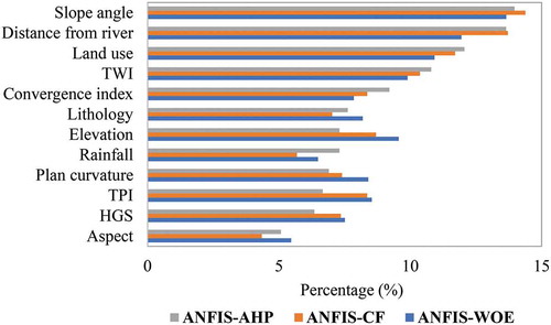
Figure 8. Map of FPI_ANFIS-AHP values across the Trotuș River basin

FPI - Flood Potential Index; ANFIS - Adaptive Neuro-Fuzzy Inference System; AHP - Analytical Hierachy Process.

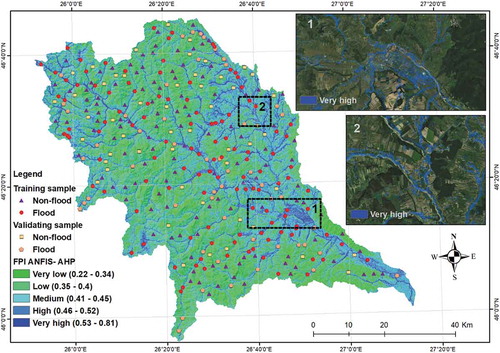
Figure 9. Map of FPI_ANFIS-CF values across the Trotuș River basin

FPI - Flood Potential Index; ANFIS - Adaptive Neuro-Fuzzy Inference System; CF - Certainty Factor.

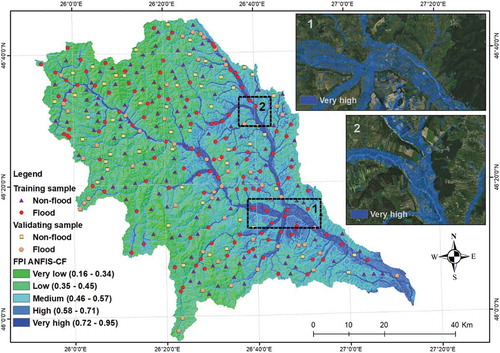
Figure 10. Weights of the FPI classes

FPI - Flood Potential Index; ANFIS - Adaptive Neuro-Fuzzy Inference System; AHP - Analytical Hierarchy Process; CF - Certainty Factor; WOE - Weights of Evidence.

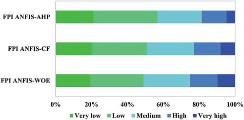
Figure 11. Map of FPI_ANFIS-WOE values across the Trotuș River basin

FPI - Flood Potential Index; ANFIS - Adaptive Neuro-Fuzzy Inference System; WOE - Weights of Evidence.

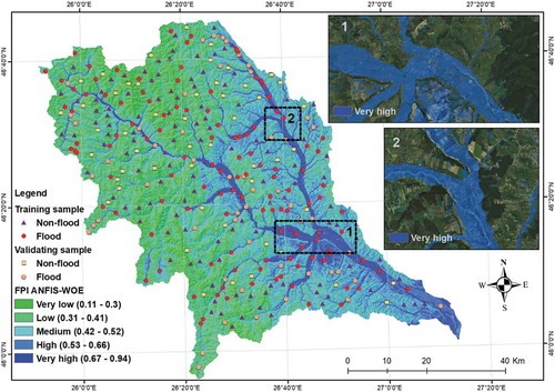
The multiplication of the relative importance with the values of WOE coefficients allowed the derivation of FPI_ANFIS-WOE throughout the study area. The range of values between 0.11 and 0.94 was divided into five classes by the natural breaks method. The first class of FPI_ANFIS-WOE values (0.11–0.3) covers about 19.43% of the study area, while the low values class (0.31–0.41) covers 29.56%. The middle values extend over more than a quarter of the river basin (25.87%), while the large and very large values together cover about 25.13% (Fig. 11).

5.5 Performance validation

5.5.1 ROC curve

The first method used to validate the results is the ROC curve. The success rate was computed with the help of the training samples. Meanwhile, the prediction rate was estimated with the help of the validation samples. In terms of the success rate, the best performing model was ANFIS-CF (AUC = 0.947), followed by ANFIS-WOE (AUC = 0.932) and ANFIS-AHP (AUC = 0.930) (Fig. 12(a)). The good success rate demonstrates that most flood locations were classified in areas of high and very high flood susceptibility. In contrast, the non-flood locations are classified into very low and low flood susceptibility. In terms of the prediction rate, the ANFIS-CF (AUC = 0.892) model was also the best performing model, followed by ANFIS-AHP (AUC = 0.887) and ANFIS-WOE (AUC = 0.882) (Fig. 12(b)).

Figure 12. ROC curves: (a) success rate and (b) prediction. AUC: area under curve

ANFIS - Adaptive Neuro-Fuzzy Inference System; AHP - Analytical Hierarchy Process; CF - Certainty Factor; WOE - Weights of Evidence; AUC - Area Under Curve.

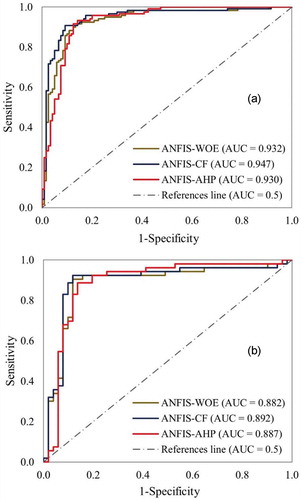
Analysing the obtained results, we can state that all three ensemble models achieved very good results in both the training dataset and the validation dataset. As in the case of the success rate, the AUC results of the prediction rate are explained by the presence of flood locations from the validation dataset in areas with high and very high flood susceptibility. The distribution of flood points within FPI classes is exemplified in the next section.

5.5.2 Flood point distribution within FPI classes

The second method used to validate the results is the estimation of the percentage of flood pixels within the FPI classes. As Table 7 indicates, in terms of the training sample, the highest presence (91.6%) of flood locations within the high and very high FPI classes belongs to the ANFIS-WOE hybrid model, followed by the ANFIS-CF hybrid model (90.9%) and the ANFIS-AHP hybrid model (84.1%). Regarding the validation sample, the highest performance was obtained also by the ANFIS-WOE hybrid model (92.4%), followed by the ANFIS-CF (88.4%) hybrid model and the ANFIS-AHP hybrid model (88.4%) (Table 7).

Table 7. Flood point distribution (%) within FPI classes

Sample	Class	ANFIS-AHP	ANFIS-CF	ANFIS-WOE
Training	Very low	0.0	0.8	1.7
	Low	4.2	0.8	1.7
	Medium	11.7	7.5	5.0
	High	30.0	16.7	22.4
	Very high	54.1	74.2	69.2
Validation	Very low	0.0	1.9	0.0
	Low	6.9	3.8	3.8
	Medium	12.8	5.8	3.8
	High	24.8	19.3	25.1
	Very high	55.5	69.2	67.3

FPI - Flood Potential Index; ANFIS - Adaptive Neuro-Fuzzy Inference System; AHP - Analytical Hierarchy Process; CF - Certainty Factor; WOE - Weights of Evidence.

6 Discussion

It is a fact that Romania, along with many other parts of the world, is increasingly affected by flood phenomena (Vinke-de Kruijf et al. 2015, Costache and Bui 2020, Costache et al. 2020b). One of Romania’s most exposed areas to flood phenomena is the Trotuș River basin. This basin was affected many times by severe flood hazard events during the last 5 years (Tincu et al. 2018). Given this fact, flood susceptibility maps with high accuracy are crucial for the local authorities. In previous work, Tincu et al. (2018) evaluated the flood susceptibility at the Trotuș River catchment using a Modified Flash Flood Potential Index (MFFPI); however, they focused only on the upper part. The MFFPI is critical because weights for generating susceptibility maps were based on expert judgement only that are somewhat objective.

Nevertheless, the results of the present research support the finding of Tincu et al. (2018) that the main river valleys at the upper part of the Trotuș River basin have the highest susceptibility to floods. Costache et al. (2020a) pointed out that between 21.88% and 36.53% of the Trotuș River basin has a high or very high flood susceptibility, while in the present study, these values range from 18.6% (FPI_ANFIS-AHP) to 25.13%. In terms of the accuracy of the results, the ANFIS-based models used here have higher accuracy than the models proposed by Costache et al. (2020a).

For the Romania territory, ANFIS, as a stand-alone model, was applied in a previous study by Costache (2019c), who analysed the flood susceptibility across the Prahova river catchment. The accuracy of the results in terms of the training data was 90.9%, while in terms of the validating sample it was 0.89. The ANFIS-based models for flood susceptibility assessment have also been used in other countries. For example, Tien Bui et al. (2018) assessed the flood susceptibility across the Haraz River basin in Iran, using ANFIS along with three optimization algorithms. In that case, the accuracy of the ANFIS hybrid models reached 94.4%. Another study, in which ANFIS was combined with two artificial intelligence algorithms, was conducted by Bui et al. (2018). In the present study, the highest accuracy was 94.7%. Therefore, in the present research, the accuracy of the ANFIS ensembles was in line with the results reported in the literature.

7 Conclusions

In the context of the continued increase in the severity and intensity of floods across the Trotuș River basin, this study proposed the application of three hybrid models to assess susceptibility to these phenomena. Research on the risk of these phenomena is becoming more and more critical. Based on the findings of this study, some conclusions can be drawn as follows:

• ANFIS is a powerful data-driven model for flood susceptibility mapping; however, the performance of the ANFIS model is dependent on how the input factors are coded. Therefore, pre-processing and coding the flood factors should be carried out properly.

The high performance of the three ensemble models (ANFIS-AHP, ANFIS-CF, ANFIS-WOE) in this study indicates that AHP, CF and WOE are appropriate techniques for translating categorical variables into numeric variables for flood modelling.

• Using these three hybrid models to calculate flood susceptibility has not previously been explored in the literature and represents the main novelty of the present study. These models, which are characterized by very high accuracy and performance, can represent an essential reference for future studies carried out by other researchers.

• The present analysis is also important in practical terms: once the flood-prone areas are identified, appropriate measures to reduce the adverse effects of these phenomena can be taken. The results of the present paper can be used in the hydrological forecasting activity.

Disclosure statement

No potential conflict of interest was reported by the authors.

References

- Abedini, M., et al., 2019. A comparative study of support vector machine and logistic model tree classifiers for shallow landslide susceptibility modeling. Environmental Earth Sciences, 78 (18), 560. doi:10.1007/s12665-019-8562-z
- Adhikari, P., et al., 2010. A digitized global flood inventory (1998–2008): compilation and preliminary results. Natural Hazards, 55 (2), 405–422. doi:10.1007/s11069-010-9537-2
- Ahmadlou, M., et al., 2019. Flood susceptibility assessment using integration of adaptive network-based fuzzy inference system (ANFIS) and biogeography-based optimization (BBO) and BAT algorithms (BA). Geocarto International, 34 (11), 1252–1272.
- Alfieri, L., et al., 2018. Multi-model projections of river flood risk in Europe under global warming. Climate, 6 (1), 6. doi:10.3390/cli6010006
- Ali, S.A., et al., 2020. GIS-based comparative assessment of flood susceptibility mapping using hybrid multicriteria decision-making approach, naïve Bayes tree, bivariate statistics and logistic regression: a case of Topľa basin, Slovakia. Ecological Indicators, 117, 106620. doi:10.1016/j.ecolind.2020.106620
- Ameri, A.A., Pourghasemi, H.R., and Cerda, A., 2018. Erodibility prioritization of sub-watersheds using morphometric parameters analysis and its mapping: a comparison among TOPSIS, VIKOR, SAW, and CF multicriteria decision making models. Science of the Total Environment, 613, 1385–1400. doi:10.1016/j.scitotenv.2017.09.210
- Avand, M., et al., 2020. A tree-based intelligence ensemble approach for spatial prediction of potential groundwater. International Journal of Digital Earth, 1–22. doi:10.1080/17538947.2020.1718785
- Azareh, A., et al., 2019. Incorporating multicriteria decision-making and fuzzy-value functions for flood susceptibility assessment. Geocarto International, 1–21. doi:10.1080/10106049.2019.1695958
- Below, R. and Wallemacq, P., 2018. Natural disasters 2017. Brussels: Centre for Research on the Epidemiology of Disasters (CRED).
- Bodoque, J.M., et al., 2019. Enhancing flash flood risk perception and awareness of mitigation actions through risk communication: a pre-post survey design. Journal of Hydrology, 568, 769–779. doi:10.1016/j.jhydrol.2018.11.007
- Bolt, B.A., et al., 2013. Geological hazards: earthquakes-tsunamis-volcanoes-avalanches-landslides-floods. Springer Science & Business Media, Springer-Verlag Berlin Heidelberg.
- Brunner, G.W., 1995. HEC-RAS river analysis system. Hydraulic reference manual. Version 1.0. Davis, CA: Hydrologic Engineering Center.
- Bui, D.T., et al., 2016. Hybrid artificial intelligence approach based on neural fuzzy inference model and metaheuristic optimization for flood susceptibilitgy modeling in a high-frequency tropical cyclone area using GIS. Journal of Hydrology, 540, 317–330. doi:10.1016/j.jhydrol.2016.06.027
- Bui, D.T., et al., 2018. Novel hybrid evolutionary algorithms for spatial prediction of floods. Scientific Reports, 8 (1), 15364. doi:10.1038/s41598-018-33755-7
- Bui, D.T., et al., 2019a. A new intelligence approach based on GIS-based multivariate adaptive regression splines and metaheuristic optimization for predicting flash flood susceptible areas at high-frequency tropical typhoon area. Journal of Hydrology, 575, 314–326. doi:10.1016/j.jhydrol.2019.05.046
- Bui, D.T., et al., 2019b. Flash flood susceptibility modeling using an optimized fuzzy rule based feature selection technique and tree based ensemble methods. Science of the Total Environment, 668, 1038–1054. doi:10.1016/j.scitotenv.2019.02.422
- Bui, D.T., et al., 2020. A novel deep learning neural network approach for predicting flash flood susceptibility: a case study at a high frequency tropical storm area. Science of the Total Environment, 701, 134413. doi:10.1016/j.scitotenv.2019.134413
- Celikyilmaz, A. and Turksen, I.B., 2009. Modeling uncertainty with fuzzy logic. Studies in Fuzziness and Soft Computing, 240, 149–215.
- Chapi, K., et al., 2017. A novel hybrid artificial intelligence approach for flood susceptibility assessment. Environmental Modelling & Software, 95, 229–245. doi:10.1016/j.envsoft.2017.06.012
- Choubin, B., et al., 2019. An ensemble prediction of flood susceptibility using multivariate discriminant analysis, classification and regression trees, and support vector machines. Science of the Total Environment, 651, 2087–2096. doi:10.1016/j.scitotenv.2018.10.064
- Corsini, A., Cervi, F., and Ronchetti, F., 2009. Weight of evidence and artificial neural networks for potential groundwater spring mapping: an application to the Mt. Modino area (Northern Apennines, Italy). Geomorphology, 111 (1–2), 79–87. doi:10.1016/j.geomorph.2008.03.015
- Costa, V. and Fernandes, W., 2017. Bayesian estimation of extreme flood quantiles using a rainfall-runoff model and a stochastic daily rainfall generator. Journal of Hydrology, 554, 137–154. doi:10.1016/j.jhydrol.2017.09.003
- Costache, R., 2014a. Assessing monthly average runoff depth in Sărățel river basin, Romania. Analele stiintifice ale Universitatii” Alexandru Ioan Cuza” Din Iasi-seria Geografie, 60 (1), 97–110.
- Costache, R., 2014b. Estimating multiannual average runoff depth in the middle and upper sectors of Buzău River basin. Geographia Technica, 9 (2), 21–29.
- Costache, R., et al., 2015. Flood vulnerability assessment in the low sector of Saratel catchment. Case study: Joseni village. Carpathian Journal of Earth and Environmental Sciences, 10 (1), 161–169.
- Costache, R., 2019a. Flash-flood potential index mapping using weights of evidence, decision trees models and their novel hybrid integration. Stochastic Environmental Research and Risk Assessment, 33 (7), 1375–1402. doi:10.1007/s00477-019-01689-9
- Costache, R., 2019b. Flash-flood potential assessment in the upper and middle sector of Prahova river catchment (Romania). A comparative approach between four hybrid models. Science of the Total Environment, 659, 1115–1134. doi:10.1016/j.scitotenv.2018.12.397
- Costache, R., 2019c. Flood susceptibility assessment by using bivariate statistics and machine learning models-A useful tool for flood risk management. Water Resources Management, 33 (9), 3239–3256. doi:10.1007/s11269-019-02301-z
- Costache, R., et al., 2020a. Novel hybrid models between bivariate statistics, artificial neural networks and boosting algorithms for flood susceptibility assessment, Journal of Environmental Management, 265, 110485. doi:10.1016/j.jenvman.2020.110485
- Costache, R., et al., 2020a. Using GIS, remote sensing, and machine learning to highlight the correlation between the land-use/land-cover changes and flash-flood potential. Remote Sensing, 12 (9), 1422. doi:10.3390/rs12091422
- Costache, R., et al., 2020b. Novel hybrid models between bivariate statistics, artificial neural networks and boosting algorithms for flood susceptibility assessment. Journal of Environmental Management, 265, 110485. doi:10.1016/j.jenvman.2020.110485
- Costache, R., et al., 2020c. Flash-flood susceptibility assessment using multi-criteria decision making and machine learning supported by remote sensing and GIS techniques. Remote Sensing, 12 (1), 106. doi:10.3390/rs12010106
- Costache, R., et al., 2020d. Spatial predicting of flood potential areas using novel hybridizations of fuzzy decision-making, bivariate statistics, and machine learning. Journal of Hydrology, 585, 124808. doi:10.1016/j.jhydrol.2020.124808
- Costache, R. and Bui, D.T., 2019. Spatial prediction of flood potential using new ensembles of bivariate statistics and artificial intelligence: a case study at the Putna river catchment of Romania. Science of the Total Environment, 691, 1098–1118. doi:10.1016/j.scitotenv.2019.07.197
- Costache, R. and Bui, D.T., 2020. Identification of areas prone to flash-flood phenomena using multiple-criteria decision-making, bivariate statistics, machine learning and their ensembles. Science of the Total Environment, 712, 136492. doi:10.1016/j.scitotenv.2019.136492
- Costache, R., Fontanine, I., and Corodescu, E., 2014. Assessment of surface runoff depth changes in Sǎrǎţel River basin, Romania using GIS techniques. Open Geosciences, 6 (3), 363–372.
- Costache, R., Hong, H., and Pham, Q.B., 2020a. Comparative assessment of the flash-flood potential within small mountain catchments using bivariate statistics and their novel hybrid integration with machine learning models. Science of the Total Environment, 711, 134514. doi:10.1016/j.scitotenv.2019.134514
- Costache, R., Hong, H., and Wang, Y., 2019. Identification of torrential valleys using GIS and a novel hybrid integration of artificial intelligence, machine learning and bivariate statistics. Catena, 183, 104179. doi:10.1016/j.catena.2019.104179
- Costache, R., Ngo, P.T.T., and Tien Bui, D., 2020b. Novel ensembles of deep learning neural network and statistical learning for flash-flood susceptibility mapping. Water, 12 (6), 1549. doi:10.3390/w12061549
- Costache, R. and Zaharia, L., 2017. Flash-flood potential assessment and mapping by integrating the weights-of-evidence and frequency ratio statistical methods in GIS environment–case study: Bâsca Chiojdului River catchment (Romania). Journal of Earth System Science, 126 (4), 59. doi:10.1007/s12040-017-0828-9
- Dodangeh, E., et al., 2020. Integrated machine learning methods with resampling algorithms for flood susceptibility prediction. Science of the Total Environment, 705, 135983. doi:10.1016/j.scitotenv.2019.135983
- Dottori, F., et al., 2018. Increased human and economic losses from river flooding with anthropogenic warming. Nature Climate Change, 8, 781–786. doi:10.1038/s41558-018-0257-z
- Dumitriu, D., 2019. Relationships between sediment transport and various hydrological and hydraulic characteristics of flood events on Trotuș River (Romania).
- El Alfy, M., 2016. Assessing the impact of arid area urbanization on flash floods using GIS, remote sensing, and HEC-HMS rainfall–runoff modeling. Hydrology Research, 47 (6), 1142–1160. doi:10.2166/nh.2016.133
- Elkhrachy, I., 2015. Flash flood hazard mapping using satellite images and GIS tools: a case study of Najran City, Kingdom of Saudi Arabia (KSA). The Egyptian Journal of Remote Sensing and Space Science, 18 (2), 261–278. doi:10.1016/j.ejrs.2015.06.007
- Fortin, J.-P., et al., 2001. Distributed watershed model compatible with remote sensing and GIS data. I: description of model. Journal of Hydrologic Engineering, 6 (2), 91–99. doi:10.1061/(ASCE)1084-0699(2001)6:2(91)
- Guha-Sapir, D., 2012. Disaster data: a balanced perspective. CredCrunch, 27, 1–2.
- Henstra, D., et al., 2019. Flood risk management and shared responsibility: exploring Canadian public attitudes and expectations. Journal of Flood Risk Management, 12 (1), e12346. doi:10.1111/jfr3.12346
- Hong, H., et al., 2018. Flood susceptibility assessment in Hengfeng area coupling adaptive neuro-fuzzy inference system with genetic algorithm and differential evolution. Science of the Total Environment, 621, 1124–1141. doi:10.1016/j.scitotenv.2017.10.114
- Hosseini, F.S., et al., 2020. Flash-flood hazard assessment using ensembles and Bayesian-based machine learning models: application of the simulated annealing feature selection method. Science of the Total Environment, 711, 135161. doi:10.1016/j.scitotenv.2019.135161
- Jang, J.-S., 1993. ANFIS: adaptive-network-based fuzzy inference system. IEEE Transactions on Systems, Man, and Cybernetics, 23 (3), 665–685. doi:10.1109/21.256541
- Khattak, M.S., et al., 2016. Floodplain mapping using HEC-RAS and ArcGIS: a case study of Kabul River. Arabian Journal for Science and Engineering, 41 (4), 1375–1390. doi:10.1007/s13369-015-1915-3
- Khosravi, K., et al., 2018. A comparative assessment of decision trees algorithms for flash flood susceptibility modeling at Haraz watershed, northern Iran. Science of the Total Environment, 627, 744–755. doi:10.1016/j.scitotenv.2018.01.266
- Khosravi, K., et al., 2019. A comparative assessment of flood susceptibility modeling using multi-criteria decision-making analysis and machine learning methods. Journal of Hydrology, 573, 311–323. doi:10.1016/j.jhydrol.2019.03.073
- Kourgialas, N.N. and Karatzas, G.P., 2011. Flood management and a GIS modelling method to assess flood-hazard areas—a case study. Hydrological Sciences Journal–Journal Des Sciences Hydrologiques, 56 (2), 212–225. doi:10.1080/02626667.2011.555836
- Kucsicsa, G., et al., 2019. Future land use/cover changes in Romania: regional simulations based on CLUE-S model and CORINE land cover database. Landscape and Ecological Engineering, 15 (1), 75–90. doi:10.1007/s11355-018-0362-1
- Kurnik, B., et al., 2017. Weather-and climate-related natural hazards in Europe. In: Climate change adaptation and disaster risk reduction in Europe. Kongens Nytorv 61050 Copenhagen K Denmark: EEA-European Environment Agency, 46–91.
- Lázaro, J.M., et al., 2016. Flood frequency analysis (FFA) in Spanish catchments. Journal of Hydrology, 538, 598–608. doi:10.1016/j.jhydrol.2016.04.058
- Lee, S., et al., 2017. Spatial prediction of flood susceptibility using random-forest and boosted-tree models in Seoul metropolitan city, Korea. Geomatics, Natural Hazards and Risk, 8 (2), 1185–1203. doi:10.1080/19475705.2017.1308971
- Linkov, I., et al., 2009. Weight-of-evidence evaluation in environmental assessment: review of qualitative and quantitative approaches. Science of the Total Environment, 407 (19), 5199–5205. doi:10.1016/j.scitotenv.2009.05.004
- Linzer, H.-G., et al., 1998. Kinematic evolution of the Romanian Carpathians. Tectonophysics, 297 (1–4), 133–156. doi:10.1016/S0040-1951(98)00166-8
- Luca, M. and Avram, M., 2017. Analysis of the hydroclimatic risk parameters at the high level of the Tazlăul Sărat river in 2016 year. Present Environment and Sustainable Development, 11 (2), 97–108. doi:10.1515/pesd-2017-0028
- Maiti, S. and Tiwari, R., 2014. A comparative study of artificial neural networks, Bayesian neural networks and adaptive neuro-fuzzy inference system in groundwater level prediction. Environmental Earth Sciences, 71 (7), 3147–3160. doi:10.1007/s12665-013-2702-7
- Masseroni, D., et al., 2017. A reliable rainfall–runoff model for flood forecasting: review and application to a semi-urbanized watershed at high flood risk in Italy. Hydrology Research, 48 (3), 726–740. doi:10.2166/nh.2016.037
- Moradi, H., Avand, M.T., and Janizadeh, S., 2019. Landslide susceptibility survey using modeling methods. In: Hamid Pourghasemi Candan Gokceoglu, eds. Spatial modeling in GIS and R for earth and environmental sciences. Elsevier, 259–275.
- Mosavi, A., Ozturk, P., and Chau, K., 2018. Flood prediction using machine learning models: literature review. Water, 10 (11), 1536. doi:10.3390/w10111536
- Nandi, A., et al., 2016. Flood hazard mapping in Jamaica using principal component analysis and logistic regression. Environmental Earth Sciences, 75 (6), 465. doi:10.1007/s12665-016-5323-0
- Ngo, P.-T., et al., 2018. A novel hybrid swarm optimized multilayer neural network for spatial prediction of flash floods in tropical areas using sentinel-1 SAR imagery and geospatial data. Sensors, 18 (11), 3704. doi:10.3390/s18113704
- Nguyen, P.T., et al., 2016. A high resolution coupled hydrologic–hydraulic model (HiResFlood-UCI) for flash flood modeling. Journal of Hydrology, 541, 401–420. doi:10.1016/j.jhydrol.2015.10.047
- Nguyen, V.-N., et al., 2017. An integration of least squares support vector machines and firefly optimization algorithm for flood susceptible modeling using GIS. Presented at the International Conference on Geo-Spatial Technologies and Earth Resources, Hanoi, Vietnam: Springer, 52–64.
- Nhu, V.-H., et al., 2020. Gis-based gully erosion susceptibility mapping: a comparison of computational ensemble data mining models. Applied Sciences, 10 (6), 2039. doi:10.3390/app10062039
- Oh, H.-J. and Pradhan, B., 2011. Application of a neuro-fuzzy model to landslide-susceptibility mapping for shallow landslides in a tropical hilly area. Computers & Geosciences, 37 (9), 1264–1276. doi:10.1016/j.cageo.2010.10.012
- Pelling, M., et al., 2004. Reducing disaster risk: a challenge for development.. New York, NY, USA: United Nations Development Programme Bureau for Crisis Prevention and Recovery One United Nations Plaza.
- Petrow, T. and Merz, B., 2009. Trends in flood magnitude, frequency and seasonality in Germany in the period 1951–2002. Journal of Hydrology, 371 (1–4), 129–141. doi:10.1016/j.jhydrol.2009.03.024
- Pham, B.T., et al., 2020. GIS based hybrid computational approaches for flash flood susceptibility assessment. Water, 12 (3), 683. doi:10.3390/w12030683
- Pham, Q.B., et al., 2019. Potential of hybrid data-intelligence algorithms for multi-station modelling of rainfall. Water Resources Management, 33 (15), 5067–5087. doi:10.1007/s11269-019-02408-3
- Prăvălie, R. and Costache, R., 2013. The vulnerability of the territorial-administrative units to the hydrological phenomena of risk (flash-floods). Case study: the subcarpathian sector of Buzău catchment. Analele Universității Din Oradea–Seria Geografie, 23 (1), 91–98.
- Prăvălie, R. and Costache, R., 2014a. The potential of water erosion in Slănic River basin. Revista de Geomorfologie, 16, 79–88.
- Prăvălie, R. and Costache, R., 2014b. The analysis of the susceptibility of the flash-floods’ genesis in the area of the hydrographical basin of Bāsca Chiojdului river/Analiza susceptibilitatii genezei viiturilor īn aria bazinului hidrografic al rāului Bāsca Chiojdului. Forum Geografic, 13 (1), 39–49. doi:10.5775/fg.2067-4635.2014.071.i
- Rahmati, O. and Pourghasemi, H.R., 2017. Identification of critical flood prone areas in data-scarce and ungauged regions: a comparison of three data mining models. Water Resources Management, 31 (5), 1473–1487. doi:10.1007/s11269-017-1589-6
- Regmi, N.R., Giardino, J.R., and Vitek, J.D., 2010. Modeling susceptibility to landslides using the weight of evidence approach: Western Colorado, USA. Geomorphology, 115 (1–2), 172–187. doi:10.1016/j.geomorph.2009.10.002
- Saaty, T.L., 1980. The analytical hierarchy process, planning, priority. Resource allocation. USA: RWS publications.
- Sarhadi, A., Soltani, S., and Modarres, R., 2012. Probabilistic flood inundation mapping of ungauged rivers: linking GIS techniques and frequency analysis. Journal of Hydrology, 458, 68–86. doi:10.1016/j.jhydrol.2012.06.039
- Shortliffe, E.H. and Buchanan, B.G., 1975. A model of inexact reasoning in medicine. Mathematical Biosciences, 23 (3–4), 351–379. doi:10.1016/0025-5564(75)90047-4
- Skaugen, T. and Onof, C., 2014. A rainfall‐runoff model parameterized from GIS and runoff data. Hydrological Processes, 28 (15), 4529–4542. doi:10.1002/hyp.9968
- Skaugen, T., Peerebom, I.O., and Nilsson, A., 2015. Use of a parsimonious rainfall–run‐off model for predicting hydrological response in ungauged basins. Hydrological Processes, 29 (8), 1999–2013. doi:10.1002/hyp.10315
- Talukdar, S., et al., 2020. Flood susceptibility modeling in Teesta River basin, Bangladesh using novel ensembles of bagging algorithms. Stochastic Environmental Research and Risk Assessment, 1–24. doi:10.1007/s00477-020-01862-5
- Tanwattana, P., 2018. Systematizing community-based disaster risk management (CBDRM): case of urban flood-prone community in Thailand upstream area. International Journal of Disaster Risk Reduction, 28, 798–812. doi:10.1016/j.ijdrr.2018.02.010
- Tehrany, M.S., et al., 2014. Flood susceptibility mapping using integrated bivariate and multivariate statistical models. Environmental Earth Sciences, 72 (10), 4001–4015. doi:10.1007/s12665-014-3289-3
- Tehrany, M.S., et al., 2015. Flood susceptibility assessment using GIS-based support vector machine model with different kernel types. Catena, 125, 91–101. doi:10.1016/j.catena.2014.10.017
- Tehrany, M.S., Pradhan, B., and Jebur, M.N., 2014. Flood susceptibility mapping using a novel ensemble weights-of-evidence and support vector machine models in GIS. Journal of Hydrology, 512, 332–343.
- Teng, J., et al., 2017. Flood inundation modelling: a review of methods, recent advances and uncertainty analysis. Environmental Modelling & Software, 90, 201–216. doi:10.1016/j.envsoft.2017.01.006
- Termeh, S.V.R., et al., 2018. Flood susceptibility mapping using novel ensembles of adaptive neuro fuzzy inference system and metaheuristic algorithms. Science of the Total Environment, 615, 438–451. doi:10.1016/j.scitotenv.2017.09.262
- Tien Bui, D., et al., 2018. New hybrids of anfis with several optimization algorithms for flood susceptibility modeling. Water, 10 (9), 1210. doi:10.3390/w10091210
- Tincu, R., Lazar, G., and Lazar, I., 2018. Modified flash flood potential index in order to estimate areas with predisposition to water accumulation. Open Geosciences, 10 (1), 593–606. doi:10.1515/geo-2018-0047
- Vinke-de Kruijf, J., Kuks, S.M., and Augustijn, D.C., 2015. Governance in support of integrated flood risk management? The case of Romania. Environmental Development, 16, 104–118. doi:10.1016/j.envdev.2015.04.003
- Wang, Y., et al., 2019a. A hybrid GIS multi-criteria decision-making method for flood susceptibility mapping at Shangyou, China. Remote Sensing, 11 (1), 62. doi:10.3390/rs11010062
- Wang, Y., et al., 2019b. Flood susceptibility mapping in Dingnan County (China) using adaptive neuro-fuzzy inference system with biogeography based optimization and imperialistic competitive algorithm. Journal of Environmental Management, 247, 712–729. doi:10.1016/j.jenvman.2019.06.102
- Wod, I., 1985. Weight of evidence: a brief survey. Bayesian Statistics, 2 (2), 249–270.
- Xu, L., et al., 2013. Research on the triggering factors analysis and relevant countermeasures of FaTing mountain landslide induced by Wenchuan earthquake. In: Earthquake-Induced Landslides. Springer Berlin Heidelberg, 355–365.
- Yan, L., et al., 2017. Frequency analysis of nonstationary annual maximum flood series using the time‐varying two‐component mixture distributions. Hydrological Processes, 31 (1), 69–89. doi:10.1002/hyp.10965
- Yariyan, P., et al., 2020a. Earthquake vulnerability mapping using different hybrid models. Symmetry, 12 (3), 405.
- Yariyan, P., et al., 2020b. Improvement of best first decision trees using bagging and dagging ensembles for flood-risk mapping. Water Resources Management, 34 (9), 3037–3053. doi:10.1007/s11269-020-02603-7
- Zaharia, L., et al., 2015. Assessment and mapping of flood potential in the Slănic catchment in Romania. Journal of Earth System Science, 124 (6), 1311–1324. doi:10.1007/s12040-015-0608-3
- Zaharia, L., et al., 2017. Mapping flood and flooding potential indices: a methodological approach to identifying areas susceptible to flood and flooding risk. Case study: the Prahova catchment (Romania). Frontiers of Earth Science, 11 (2), 229–247. doi:10.1007/s11707-017-0636-1
- Zhao, G., et al., 2019. Assessment of urban flood susceptibility using semi-supervised machine learning model. Science of the Total Environment, 659, 940–949. doi:10.1016/j.scitotenv.2018.12.217
- Zhou, Q., et al., 2012. Framework for economic pluvial flood risk assessment considering climate change effects and adaptation benefits. Journal of Hydrology, 414, 539–549. doi:10.1016/j.jhydrol.2011.11.031
- Zuo, R., et al., 2015. Evaluation of uncertainty in mineral prospectivity mapping due to missing evidence: a case study with skarn-type Fe deposits in Southwestern Fujian Province, China. Ore Geology Reviews, 71, 502–515. doi:10.1016/j.oregeorev.2014.09.024