Mapping abrupt streamflow shift in an abrupt climate shift through multiple change point methodologies: Brazil case study

ABSTRACT

Three change-point methodologies were used to detect changes in the mean value of annual streamflow series and analyse simultaneous changes in large-scale global sea surface temperature (SST) oscillations. To verify the relationship between the variables we used wavelet coherence analysis. A preliminary detection skill test was performed using asynthetic series and Pruned Exact Linear Time (PELT) presented the best results among the methods used (Pettitt test, Bai and Perron algorithm) when combined with a penalty selection via the Changepoints for a Range of Penalties (CROPS) method. However, the use of classical penalty functions resulted in a poor performance of PELT. The three methods showed an extremely high convergence rate (> 90%) for the correct change points and a smaller rate for false positives (< 24%). Changes in the streamflow mean value coincided with phase shift of the low-frequency indices Atlantic Multidecadal Oscillation (AMO) and Pacific Decadal Oscillation (PDO), also corroborated by the wavelet results. Most of the changes can be associated with phase shift impacts in the South Atlantic Convergence Zone.

KEYWORDS:

• change point analysis
• streamflow
• Atlantic multidecadal oscillation
• Pacific decadal oscillation
• El Niño

Editor A. Castellarin Associate editor X. Sun

Introduction

The variability of sea surface temperature (SST) at different oscillation scales, such as interannual, decadal and multi-decadal, is considered one of the drivers behind changes in hydrologic variables (Kayano and Andreoli 2007, Kayano and Capistrano 2014, Tang et al. 2014, Wang et al. 2018). Understanding in detail the different periodic SST cycles and their effects on hydrologic variables can improve climate-based forecast models and water granting policies, and also provides better predictability to water resources system management, enhancing its resilience.

Approaches ranging from the use of artificial intelligence to periodic regression models incorporate SST indices in streamflow forecasting (Souza Filho and Lall 2003, Block et al. 2009, Sankarasubramanian et al. 2009, Lima and Lall 2010a, Fritier et al. 2012, Bradley et al. 2015, Lehner et al. 2017, Yang et al. 2017). Selecting the correct indices in climate-based forecasting is based on the knowledge of either the physical or the statistical relationship of the phenomenon and the streamflow.

One classical approach is to base the selection in correlation coefficients and develop a single equation to represent the streamflow behaviour (Lima and Lall 2010a). However, different phases of periodic cycles of the Atlantic and Pacific oceans can possibly modify the behaviour of the streamflow and affect the series’ statistical properties, increasing the complexity of the model required to correctly incorporate these changes.

The non-stationarity present in streamflow series can pose a challenge not just to the development of climate-based forecast models but, more importantly, to water systems management. Periods with diverging mean values impose either changes in water granting policies, to adjust the values to the reality faced, or a high opportunity cost generated from a conservative policy that uses a fixed low streamflow value as the basis for the granting policies. Also, different variance periods can either increase or decrease uncertainties, which in turn affects the risk associated with water allocation. Thus, the mean and the variance are the two fundamental statistical properties that define the possible water management policies.

Many recent articles uses change-point analysis to detect changes in the statistical properties of the streamflow series using diverse methodologies (Ivancic and Shaw 2017, Zhang et al. 2019, Ryberg et al. 2019). To explore the relationship between the changes detected in streamflow series and climate indices, Tamaddun et al. (2019) used cross wavelet analysis (XTC) and wavelet coherency analysis (WTC), and found that significant shifts occurred during the coupled phases of the climate signals. The use of XTC and WTC to investigate the influence of climate indices in hydroclimatic variables can be found in diverse studies, with solid results (Tang et al. 2014, Tamaddun et al. 2017a, 2017b, Rocha et al. 2019). However, we have not found other studies using change-point analysis to identify phase shifts of climate indices and to match change points in streamflow time series.

Despite the numerous change-point methodologies found in the literature, the discovery of whether a change occurs in a time series and its true location is still an open question, since different methodologies impose diverging results. This problem is amplified with the use of methods based either on likelihood cost-functions that are strongly dependent on the penalty selection (where a high value for the penalty inhibits the change detection and low values impose a great number of false positives) or on methods with a predefined number of change points. These particularities results in a more subjective analysis. Therefore, more studies are needed to provide reliability to the change-point results and to explore the usability of classical penalty functions or other predefinition strategies, specifically for change-point detection in hydroclimatic variables.

In this study we detected and analysed changes in the mean value of 88 Brazilian naturalized streamflow series and searched for associations with changes detected in the mean values of climate SST indices. To accomplish this task, a preliminary complementary study was performed to assess the detection skill and resulting convergence of three change-point methodologies with the use of synthetic series already employed in a previous study (Ryberg et al. 2019). The methods used here were the Pettitt test (non-parametric), the pruned exact linear time method (PELT; parametric version, likelihood cost-function based), and the dynamic algorithm proposed by Bai and Perron (2003) to estimate change points in time series regression models. WTC was also used to verify the associations between the changes observed and the SST indices.

Case study background

The streamflow series is of major importance to the Brazilian hydropower system, since it is the country’s main power source, accounting for 66.6% of its total energy supply (636.4 TWh) (Ministry of Mines and Energy, 2019). Brazil’s continental size also enables a spatial analysis that encompasses regions with diverse climate behaviour, where the atmosphere–ocean dynamic imposes different local impacts.

In recent years, a reduction in the inflow from hydroelectric power basins located in the country’s Northeast region was reported by the Electric System National Operator (ONS). A technical report of Brazil’s National Water Management Agency (ANA) also identified a reduction in 80% of 125 rainfall monitoring stations (ANA, 2013), which can explain the observed reduction in inflow by a corresponding reduction in precipitation. However, a different behaviour was reported for the South and Southeast regions, which saw a precipitation increase. Due to the magnitude of the changes reported, this study focused on evaluating large-scale global phenomena.

Castro et al. (2013) indicate a possible relationship between low-frequency SST oscillation and variation patterns observed in ONS streamflow time series. A possible association between the inflow changes mentioned and a low-frequency periodic phenomenon suggest that this occurrence is not a punctual event that occurs in an abnormal year but instead a periodic behaviour with a long-lasting effect, with significant impacts on energy production. Also, these characteristics demand a system of water management capable of responding the associated dynamic climate risk.

Thus, the Atlantic Multidecadal Oscillation (AMO) and Pacific Decadal Oscillation (PDO) indices were selected to represent the low-frequency SST oscillations, due to studies that impose a relationship between these indices and rainfall in Brazil and South America (Kayano and Andreoli 2007, Kayano and Capistrano 2014, Rocha et al. 2019). The El Niño index was used because its phenomenal impact on Brazilian rainfall has already been extensively reported, and it is the main index used in Brazilian streamflow forecast models.

Data and methodology

Case study data and teleconnections

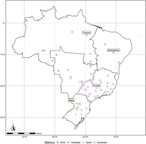
Monthly data of naturalized streamflow was used. We had access to data from 1931 to 2016, taken from 88 stations grouped in four regions distributed throughout Brazil, following the ONS standard (Fig. 1). These regions diverge from the geographical division due to the operational relationships between hydropower dams.

Figure 1. Location of streamflow stations. Key stations are highlighted (triangles) and labelled. The stations colour represents its region according to ONS standards

The naturalized flows were acquired after a process of consolidation and consistency of the measurements from streamflow gauges and the account of anthropogenically derived factors: reservoir operations upstream of the streamflow, evaporation of the reservoir, water withdrawal along the basins, river flow alterations due to infrastructure built along a natural course, and operational pumping. Details of these processes can be found in ONS (2017). Annual streamflow series were obtained by averaging monthly values.

Four key stations (highlighted in Fig. 1) were selected for a more extensive analysis due to their relevance: Furnas, Sobradinho, Tucuruí and Itaipu. Itaipu is the world’s second largest hydropower dam in terms of electricity production, with an installed capacity of 14 000 MW, accounting for 15% of the energy used in Brazil and 90% of the energy used in Paraguay. Tucuruí is the largest exclusively Brazilian hydropower plant with a capacity of 8370 MW, being the main source of electricity for the North subsystem. Furnas is one of the most important dams for the southeast region due to its location close to three large capitals (Rio de Janeiro, São Paulo, and Belo Horizonte) with intensive energy demand, and its high potential for energy generation (1216 MW). Sobradinho is a dam with one of the world’s largest flooded areas; it has an installed capacity of 1050.3 MW, and also has a local regularization purpose for the São Francisco River.

The indices AMO, PDO, and Niño 3.4 were acquired from the US National Oceanic and Atmospheric Administration (NOAA) database through the Working Group on Surface Pressure website (https://www.esrl.noaa.gov/psd/gcos_wgsp/Timeseries/, data retrieved in july of 2018) (Enfield et al., 2001, Mantua et al., 1997, Rayner et al., 2003).

El Niño Southern Oscillation (ENSO) is considered the most relevant oceanic–atmospheric mode of interannual climate variability on a global scale (Kayano et al. 2016). El Niño’s influence on South America’s rainfall is the result of alterations in the Walker and Hadley circulation cells. The Niño 3.4 index is calculated by averaging SST values over the region delimited by latitudes 5°N–5°S and longitudes 170–120°W, considered a key region for analysing the ENSO-related coupled ocean interactions. This index is provided with or without removing the mean value from the 1981–2000 period; in this work, the anomaly version was used.

PDO is the principal component of the SST variability of the Pacific Ocean. The homonymous index measures the anomaly of North Pacific SST intensity by the number of standard deviations from the historical mean values (Mantua et al. 1997). PDO variability is appointed as behaving symmetrically with interdecadal climatic fluctuations in the North and South hemispheres, having a particular influence in both South and North America (Castro et al. 2013). According to Kayano & Andreoli (2007), PDO modulates ENSO influence on South American rainfall, with ENSO showing stronger (or weaker) teleconnection with the rainfall according to phase convergence (or divergence) between the two oscillation modes. Castro et al. (2013) verified a positive correlation between the index and step changes observed in a series of maximum daily streamflow. Therefore, PDO influence on streamflow series is expected in the region.

AMO is considered the primary low-frequency variability mode of the Atlantic Ocean. The index is based on the mean SST anomaly of the North Atlantic (0°), calculated by removing climate change-derived interference through series detrending (Enfield et al. 2001). The index is available in two forms (with or without the use of a 10-year moving average smoothing). In this work, we used the index without smoothing. According to Kayano and Capistrano (2014), ENSO extremes are related to AMO, with stronger El Niño (La Niña) events in the cold (warm) phase of AMO. Thus, ENSO-related precipitation anomalies are amplified with phase divergence between the two phenomena (PDO and AMO).

Preliminary detection skill assessment

Ryberg et al. (2019) generated sythetic series with random change points to assess the detection skill of eight detection methods. The series were based in peak-streamflow series of six US streamgauges and consist of 600 series with one change point and 600 series with two change points (that can be reproduced using Ryberg et al.’s R code).

In this same work, Ryberg et al. (2019) found that for the mean value detection the parametric methods used did not perform well, and other non-parametric methods were discarded due to the unacceptable number of false positives; they concluded that Pettitt’s test is the most appropriate method for change-point analysis of peak streamflows. We suspected, however, that the use of the parametric PELT method (R. Killick et al. 2012) combined with the modified Bayesian information criterion (MBIC) classical penalty function could produce exceedingly high penalty values, inhinbiting the detection of the change points.

Thus, we decided to revisit and extend the results obtained by Ryberg et al. (2019) for the parametric PELT methodology, using a penalty value selected after an extensive penalty analysis. Also, we explored the convergence of results with Pettitt’s test, since it was considered the most appropriate method and was used in other recent articles for change-point detection in streamflow time series (Tamaddun et al. 2016, 2019). Since Pettitt’s test is a single-change-point detection method, we also included in the analysis the change-point detection algorithm proposed by Bai and Perron (2003), henceforth BP, which allows for the discovery of multiple points and which was not used in the work of Ryberg et al. (2019).

The convergence rate of the three methods was assessed in order to exclude eventual false positives. Following the previous work, it was considered a correct detection of the change point if it is located within 5 years of the correct year, and a base 10 logarithm was used when required to approximate normality (PELT and BP).

Pruned exact linear time and penalty selection

The PELT change-point detection methodology is an approach based on the asymptotic distribution of the likelihood ratio test to detect change points in the mean value of a sequence of normally distributed observations, and derives from Hinkley’s (1970) original paper. More recently, this methodology was extended to diverse distributions (i.e. gamma, exponential, binomial) and also for the detection of variance changes (Killick and Eckley 2013). The likelihood ratio test compares the fit quality of two models, detecting a change point when the null hypothesis of no change is rejected for the desired level of significance. Upon detecting a shift, the series is divided into two segments.

This change-point methodology resumes in the exact minimization of a cost-based equation (Killick and Eckley 2013):

(1) ${\sum }_{i=1}^{m+1}\left[C\left(y_{\left({\tau }_{i-1}\right):{\tau }_i}\right)\right]+\beta f\left(m\right)$(1)

where the first term is the sum of the likelihood cost of each segment, the second term is the penalty factor and m is the number of change points.

The cost function depends on the assumptions imposed on the statistical distribution of the observations and also on the statistical property from which changes are to be detected, given that each segment’s cost is based on its likelihood of exhibiting the statistical property.

The addition of a change point usually imposes a reduction of Equation (1)(1) ${\sum }_{i=1}^{m+1}\left[C\left(y_{\left({\tau }_{i-1}\right):{\tau }_i}\right)\right]+\beta f\left(m\right)$(1) , resulting in a natural tendency of overfitting, thus, demanding the penalty factor. The literature provides various functions to select the appropriate penalty value, e.g. the Akaike information criterion (AIC) and the Bayesian information criterion (BIC).

A more recently proposed approach is the use of a range of penalty values (changepoints for a range of penalties – CROPS), allowing the analysis of the resulting segmentation from different penalty values (Haynes et al. 2017). The CROPS algorithm finds the penalty thresholds that produce different numbers of change points from a given penalty interval. The penalty value can then be chosen by analysing graphically its value versus the number of change points, searching for an optimal or parsimonious value, e.g. a point where small variations of the penalty do not generate a significant increase in the number of change points.

For the preliminary test, the PELT method was used with all classical penalty functions provided in the R package changepoint (Killick and Eckley 2013): BIC, MBIC, AIC and Hannah-Quinn (HQ).

The penalty values from the classical penalty functions were then compared to those obtained through CROPS. For CROPS method the penalty value was obtained selecting the value that corresponded to the known number of change points or the closest higher number. The penalty behaviour was then analysed numerically to check whether the value used could be selected straightforwardly by a graphical analysis. Finally, the results obtained with the “optimal” penalty value were compared to those obtained via the other methodologies.

This framework provides the best detection skill for the combined PELT and CROPS methods, since it removes the uncertainty regarding the number of existent change points. Also, the authors’ previous knowledge of the correct number of change points would impose a likely strong bias on the penalty selection through a graphic analysis. For the present case study, CROPS was used to select the adequate penalty value when standard penalty functions did not provide satisfactory results.

Bai and Perron’s algorithm

The BP algorithm (also referred to as segment neighbourhood) selects the change points by identifying the global minimizers of the sum of squared residuals, using dynamic programming to efficiently identify the optimal partitions with varying numbers of segments. The algorithm provides discovery options for the minimum segment length and the maximum number of change points (Bai and Perron 2003, Erdman and Emerson 2007).

Through the maximum number approach, each number of change points is associated with a residual squared sum and can be combined with an information criterion to select the number of change points in the time series, either from a graphical analysis or by choosing the number that minimizes the information criterion.

The BP maximum detection performance was assessed by imposing the correct number of change points. We also evaluated the correspondence between the number of change points and the minimum value of BIC. This algorithm was used through the R package strucchange (Zeileis et al. 2002, 2003).

Pettitt test

The Pettitt test (1979) is a classical non-parametric single-change-point test for the median value, based on the Mann-Whitney U test. The change-point location is defined by the maximum value of its test statistic, and its corresponding p value is derived from a two-sided test. The test was performed using the R package trend (Pohlert 2020).

Wavelet transform and wavelet coherence analysis

The wavelet transform is used to decompose a time series into a set of high- and low-frequency functions, enabling the analysis of the multi-frequency patterns that compose the original time series. The set of functions is obtained by the dilation and translation of a mother wavelet, in the scale and time domain, respectively (Sivakumar 2017). For geophysical variables, Torrence and Compo (1998) suggest the use of the Morlet wavelet, which we also employed in this study.

The wavelet transform of two time series can be analysed via XTC, to observe the common shared power in the time-frequency space, and using WTC, to identify the relationship among spectrum bands along the time domain. XTC and WTC have been used successfully to assess the relationship between climate indices and hydroclimatic variables (Tang et al. 2014, Tamaddun et al. 2017a, 2019, Rocha et al. 2019). In this work, we focused only on the WTC results.

The WTC results refer to the wavelet squared coherence and can be analysed similarly to classical correlation. The synchronization of the wavelet phases can be assessed to analyse the incurrence of a lagged relationship between the spectrum bands of the variables. The phase difference of individual phases can be converted to an angle in the interval of [−π, π] and represented by arrows in the time-period domain plot. An absolute angle value larger than π/2 indicates that the two series move out of phase, whereas the opposite indicates an in-phase relationship. The sign of the phase difference (arrows pointing up or down) indicates which series shows the leading pattern. In this work, WTC was performed through the R package WaveletComp (Roesch and Schmidbauer 2018); more information about the methodology can be found in the work of Torrence and Webster (1999).

Results

Preliminary detection skill assessment

The penalty values for PELT from each penalty function, and the upper threshold value for CROPS, which is the highest value required to obtain the number of change points closest to the correct one, are shown in Fig. 2 for the synthetic series. It is notable that CROPS produced smaller values than those calculated by the penalty functions, where in just a few series the values ranged between AIC and HQ penalty functions, and in three series it was close to the BIC minimum value. The use of HQ and AIC resulted in the detection of change points in only a few of the time series, and when MBIC and BIC penalty functions were used, no change points were detected. MBIC resulted in the highest values; its minimum value (11.74) is almost 40% higher than the maximum obtained through CROPS (8.42), confirming the hypothesis that the use of this penalty value inhibited the change-point discovery in these series.

Figure 2. Penalty values of the synthetic series obtained from different penalty functions and CROPS method. Maximum, minimum and median values of each penalty function are shown at the bottom left, bottom right and top, respectively. CROPS maximum, minimum and median values were 6.53, 0.05 and 0.65

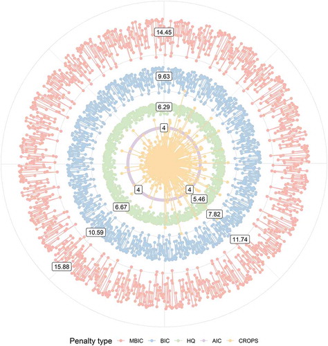
An “instantaneous” overfit pattern was noticed for the cases when the first found penalty threshold was remarkably close to zero, such as the minimum value obtained by CROPS (0.05), imposing the discovery of several change points.

The analysis of the penalty values found by CROPS for each synthetic series implies that the correct penalty could be selected through a graphical analysis, especially when the PELT algorithm successfully found the change points. Most single- and double-change-point series required a reduction ranging from 60% to 98% into the upper threshold value for the PELT algorithm to discover an extra change point. Further reductions in this decreased penalty, ranging from 20% to numbers close to 0, impose further detections, of up to five change points. This behaviour could be easily observed in a graphical analysis, where the optimal or most parsimonious value could be selected by avoiding an overfit point where small reductions in the penalty would lead to the discovery of extra change points.

However, the CROPS method could not find a penalty to produce the exact number of known change points, resulting in the presence of extra points in 27% and 24% of the single- and double-change-point series, respectively. When the methodology correctly discovers the change points the presence of extra points is reduced, i.e. to 9% and 14%. The combined PELT and CROPS successfully found 66% of the single change points, having a discovery rate of 48% for the two change points simultaneously and of 87% for at least one of the points (Table 1).

Table 1. Detection and convergence rate of Pettitt test, Bai and Perron’s algorithm and Pruned Exact Linear Time method for the synthetic series

Detection rate (%)				Convergence rate with PELT (%)
Method	Single change point	Double change points		Method	Correct change points			Incorrect change points
		All	Any		Single	Double (all)	Double (any)	Single	Double
PELT	66.17	47.83	89.00	BP	95.10	90.31	91.27	52.52	57.92
BP	57.83	37.83	88.17	Pettitt	97.79	–	97.88	20.59	25.97
Pettitt	45.33	–	39.33	BP and Pettitt	95.59	–	91.27	12.61	23.12

Similarly, BP showed a remarkably high rate of discovery of at least one of the two change points (88%), and a smaller rate of detecting the two change points (37%) simultaneously, having a 57% chance of success in the single-change-point series.

The use of BIC to select the correct number of change points worked successfully in 60% and 44% of the single- and double-change-point series, respectively. This methodology was more likely to underestimate the number of change points, since an extra change point occurred for only 2% and 3% of the series, respectively.

We obtained a success rate of 45% with the Pettitt test for the single-change-point series. This value was 3% higher than that obtained by Ryberg et al. (2019). The reason for this small difference is probably related to small differences in the random generation of the change point locations due to the use of different R versions. The R version used herein was v. 3.6.2. Even though the Pettitt test is intended to detect a single change point, it could successfully find at least one change point in 39% of the double-change-point series.

The BP and Pettitt tests presented an extremely high convergence rate with PELT for the correct change points. In the majority of cases (> 91%) when any of these methodologies successfully found the change points, PELT was also successful in finding them (Table 1). For the incorrect change points, the convergence rate was smaller. This was especially true for the three methodologies simultaneously, where an erroneous change point provided by PELT only matched the other two in 12% of the single-change-point time series. However, the convergence rate with BP for incorrect change points was higher than 55%.

These results demonstrate the superiority of the PELT and CROPS methods and indicate that the concomitant use of the three methodologies herein analysed lends more reliability to the change point results, since convergence is more likely for the correct points. For the case study, the PELT method was chosen as reference for the streamflow time series, classifying the change points according to the convergence of the methodologies. For the climate indices only the PELT method was used, and the results were compared to those in the literature.

Abrupt shift in climate indices

Preliminary tests with the penalty functions did not provide any change points for AMO and Niño 3.4. Using CROPS, it was possible to select a parsimonious value for AMO; however, for Niño 3.4 no value could be selected since the first found penalty resulted in five change points and small reductions further amplify its number, showing a overfitting pattern. This penalty behaviour means that there were no change points for Niño 3.4.

The change point analysis segmented the AMO index into three distinct phases (Fig. 3(a)): warm (from 1931 to 1963), cold (from 1964 to 1994) and warm (from 1995 to 2016). Similar results were obtained with the use of the smoothed index (Enfield et al. 2001), although with a small divergence in the phase change years. The three periods presented similar values for the standard deviation and long durations, over 20 years long (Table 2), where the shorter duration of the last period was affected by the series time window.

Table 2. Statistical properties of each segment: mean (μ), standard deviation (σ) and coefficient of variation (CV)

Index	Period	µ	σ	CV	Duration
AMO	1931–1963	0.12	0.11	0.97	33
	1964–1994	−0.17	0.12	−0.69	31
	1995–2016	0.15	0.11	0.77	22
PDO	1931 − 1943	0.66	0.81	1.21	13
	1944–1975	−0.61	0.62	−1.02	32
	1976–1998	0.57	0.64	1.11	23
	1999–2013	−0.36	0.67	−1.88	15
	2014–2016	1.44	0.27	0.19	3

Figure 3. Change point results for the mean value (bold lines) of climate indices and of the streamflow series of key stations

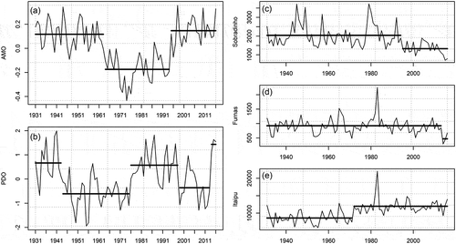
For PDO, MBIC did not result in any change points, BIC resulted in two, and both AIC and HQ produced four. With CROPS, it was noticed that AIC and HQ values were located within the optimal value interval.

The annual PDO series (Fig. 3(b)) shows five distinct phases: warm (1931–1943), cold (1944–1975), warm (1976–1998), cold (1999–2013) and warm (2014–2016). The change point years are close to those found in the literature; for example Mantua et al. (1997) mark 1947 and 1977 as PDO polarity reversal times, 3 years after the years obtained. Kayano et al. (2019) considers the period 1999–2011 a cold PDO phase, whereas Qin et al. (2018) define a cold phase between 2003 and 2014, although the authors of the latter paper state that the filtering method used influenced the period they obtained. For the time window analysed (1931–2016), the phase duration for the different indices varied between 13 and 32 years with similar absolute values of the coefficient of variation (CV; see Table 2), except for the latest period, affected by the time window used.

A warm phase convergence is notable between the PDO and AMO indices for the initial years of the series (1931–1942) and during two periods of 3 years each (1994–1997 and 2013–2016). A cold phase convergence occurred between 1964 and 1975.

Abrupt shift in streamflow series

The Sobradinho station (Fig. 3(c)) shows an accentuated reduction in the mean value for the latest years of the streamflow series, from 2044.71 to 1327.84; compared to the mean value of the complete series (1861.33) the first period value represented an increase of 9.85% whereas the latest period showed a decrease of 28.66%. Also, the last 3 years presented the series’ lowest values.

Similarly, Furnas station (Fig. 3(d)) also exhibited a significant reduction in its streamflow mean value, from 925.15 to 474, a percentual difference of 1.73% and −47.87% compared to the mean value of the series (909.41).

The Itaipu station (Fig. 3(e)), however, showed an increase in the streamflow after the change point, from 8597.09 to 11 980.08, a difference of −17% and 15% relative to the complete series mean value (10 367.26).

Figure 4 shows spatially the percentual difference between the complete series mean and the mean value of its latest change point period, also showing the convergence among the three change-point methodologies. For Sobradinho and Itaipu stations, all methodologies indicated the same change point location, whereas for Furnas, the PELT results did not converge with the other methodologies.

Figure 4. Percentage difference between the complete series mean value and the latest change point mean value, along with the convergence among the three change-point methodologies

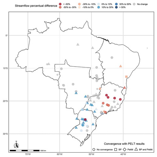
None of the methodologies used found a change point for the Tucuruí station. For the remaining northern stations, the Pettitt test indicated a change point for three western stations, where for one of these, BP also found a change point. Stations close to the north ones also did not present any change point with the use of PELT; however, for most of these stations Pettitt and BP did indicate a change point.

It is notable that the stations with streamflow reduction were localized in the eastern region of Brazil, whereas stations with the opposite behaviour were mostly concentrated near the south region. A transition zone can be seen between the stations with the opposite pattern, where mostly stations showed no change point for all the three methodologies used. The change point location obtained for the southern stations matched between the three methodologies. The PELT result for most stations with a decreasing pattern did not match the results from the other methodologies.

With regard to the penalty functions used, the classical functions did not discover any change points for most of the stations, but also imposed the discovery of a large number of change points for a few stations. Thus, the CROPS method was used to analyse and select the penalty value.

Figure 5 illustrates the indices’ mean value for each period and the percentual difference between the period mean value and the streamflow series mean value. The results are shown for each station that presented changes, grouped by ONS standards, along with the convergence between PELT and the other change-point methodologies.

Figure 5. Comparison between mean value change point results of climate indices and annual streamflow. Numbers on the right are station numbers; 168, 6 and 266 refer to the key stations Sobradinho, Furnas and Itaipu, respectively

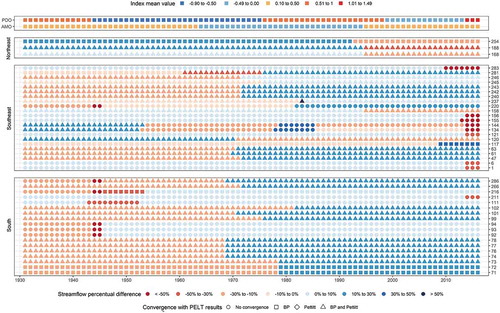
The changes detected for the northeast stations occurred in 1994 and 1992, close to the cold–warm phase shift of the AMO index, around 1994 and up to 6 years before the warm–cold phase shift of the PDO that occurred in 1998. This also occurred for southeast station 158.

It is noticeable, for the Southeast region, the presence of stations with similar streamflow reduction behaviour to Furnas (6), with an accentuated decrease in the latest years, higher than 50% for mostly stations. This also occurred for one station in the south (211). The reduction observed matches the PDO cold–warm phase shift of 2013. Two of these stations (134 and 144) presented another change point around 1980, close to the cold–warm phase shift of 1975. Also, another change was found in 1952 and 1953 – a change point location that matched among the three methodologies – but is not close to any phase shift of the indices.

Stations 281, 246 and 99 showed an increase in the change point, matching the 1980 cold–warm phase shift of the PDO, and station 281 also showed a change close to the warm–cold phase shift of the AMO; this change point location matched between BP and PELT.

Several stations presented a streamflow increase around the year 1970, including Itaipu (266). This change point location stands between phase shifts of the two indices and within the cold phase convergence of the indices. One station (120) presented the opposite pattern around the same year. Three south stations presented a change in 1978, close to the cold–warm phase shift of the PDO.

PELT detected a change point associated with low streamflow years in five south stations and one southeast station; these points, along with the periods found for stations 111 and 216, were close to the warm–cold PDO phase shift.

Figure 6 shows the results of the WTC between the key stations with change points and the AMO and PDO indices. The indices show a correlation (wavelet squared coherency) with the streamflow series for the low-frequency bands (32 to 64 years), especially for Furnas and Itaipu (> 0.8). However, the arrows indicate an opposite lag relationship between the indices’ low-frequency bands and the streamflow, with AMO out of phase and leading (arrows pointing up and left) and PDO almost in phase, showing a slight lag pattern (arrow pointing right and slightly up).

Figure 6. Wavelet coherence results between the key stations and climate indices, AMO (left) and PDO (right). The thick black contour line indicates the 5% significance level. The cone of influence is represented in white and indicates a border effect in the highlighted results

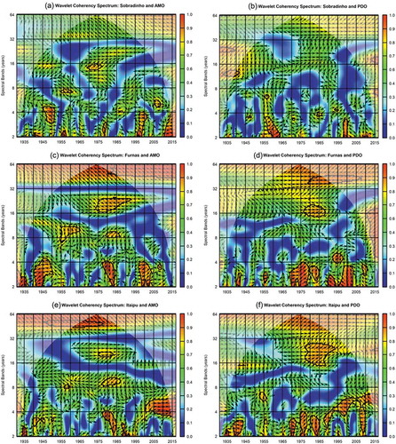
The WTC between Sobradinho and PDO (Fig. 6(b)) shows a correlation (~0.6) between the index and the streamflow for almost the complete series of spectral bands from approximately 12 to 32 years, whereas no correlation is found from 1995 to 2010, for bands from 8 to 32 years. This pattern, combined with the cold–warm phase shift of AMO, could be the reason for the change point found in 1995; also low-frequency bands showed the highest correlation in the latest years; however, these are outside the cone of influence. AMO (Fig. 6(a)) presented a more continuous influence along the complete series, except within 1950–1970 and 2000–2016 for the spectral bands of 16 to 32 years.

Furnas (Fig. 6(c) and Fig. 6(d)) presented a consistent correlation with the spectral bands of 16 to 32 years for both indices. PDO low-frequency bands presented higher values starting from 1975, where the low-frequency influence of AMO remained constant along the whole streamflow series. The latest cold–warm PDO phase shift, combined with the higher influence of PDO spectral bands from 4 to 16 years, could be the reason behind the change point observed in the latest years; however these values stand outside the cone of influence.

Itaipu (Fig. 6(d) and Fig. 6(e)) presented a consistently high correlation with the low-frequency bands of both indices, and also with PDO presenting a clearer lag pattern (arrow pointing up and right) from 1935 to 1995. Since 1965, the spectral bands from 16 to 32 years for both indices presented higher correlation values and an in-phase relationship. This pattern lasted until 1995 with AMO and for the remaining years with PDO. The leading and lagging pattern of the low-frequency bands of the indices could be one reason behind the discovery of change points in the period after the AMO phase shift of 1963 and before the PDO phase shift of 1975.

Discussion

Multi-change-point discovery performance

PELT showed good results when combined with the CROPS method to select an adequate penalty value, whereas for both the synthetic climate indices and annual streamflow time series, the penalty functions AIC, BIC, MBIC and HQ mostly inhibited change-point discovery. The overfitting pattern found to generate extra change points can be distinguished in a graphical analysis, reducing the subjectivity of the penalty selection. However, false positives were produced even when the number of change points was known, due to the impossibility of obtaining the exact number of change points, and were more common when PELT failed.

The presence of change points obtained for a period of 1 or 2 years in the case study indicates that extreme short-period events can influence change-point discovery in PELT. This observation is corroborated by Dorcas Wambui et al. (2015), who concluded that the power of the PELT method increases with the size of the change. This particularity implies that PELT failure in some of the synthetic series could be a result of small changes imposed on the synthetic time series, a hypothesis that could be confirmed by future research, since it was not analysed in this work.

Compared to the BP and the Pettitt tests, PELT presented the best performance. The convergence results showed that the use of the three methodologies combined has a small chance of converging to an erroneous change point, and a high chance of converging to the true change-point location. The combined use of just BP and PELT had a higher convergence rate for false positives. In other words, there is a clear trade-off between the overall discovery rate and the reliability of the results, since the use of multiple methodologies limits the overall performance to the worst discovery rate between the methods. The use of several methodologies to select the correct change point can be found in some previous studies (Jiménez-Ruano et al. 2017, Tongal 2019), but it is not a common practice. We find that our multi-test approach is currently the best option, since an optimum method is far from a reality. Further studies are required to improve the overall discovery rate, verify the convergence rate of different change-point methodologies and select the best complementary group of methods. The need for further studies is magnified for hydrological time series, since articles that analyse the convergence of these methods were not found in the related literature.

Case study

The spatial pattern obtained in our case study shows some similarities to the cluster results of Lima and Lall (2010b) obtained through principal component analysis, where the inflow of the reservoirs was subdivided mainly into two clusters with a transition zone cluster in between. The physical explanation given by Lima and Lall regarding the grouping of Southern Northeast and Southeast stations in the same cluster is the influence of the South Atlantic Convergence Zone (SACZ) in the rainy season. In comparison to the results obtained here, the Southeast stations show two opposite patterns and the transition zone suffered an upward right displacement, resembling more closely the spatial pattern of SACZ. This opposite pattern was already reported by Muza et al. (2009) in their analysis of extreme precipitation in South America.

The influence of AMO on the SACZ was suggested by Chiessi et al. (2009) when analysing proxy records of the discharge of La Plata River drainage basin. They concluded that during cold phases of AMO, anomalous warming of the South Atlantic would increase the activity of SACZ and displace the main belt of the South Atlantic Summer Monsoon to the south, with the opposite occurring in the warm phase of AMO. The southward displacement of the SACZ is associated with increased rainfall in southern Brazil (Barros et al. 2000) and justifies the change point location and the streamflow increase pattern found for several stations within the cold phase of AMO. The WTC results for Itaipu corroborate this conclusion, since they also show a consistent, strong low-frequency AMO influence.

The direct influence of PDO on the SACZ is not clear, but the correlation shown in the WTC of Itaipu, especially for the period starting in 1975, could be the reason why the cold–warm change of AMO did not produce another change point. The influence of PDO could be related indirectly via ENSO’s influence on SACZ. According to Cavalcanti et al. (2009), warm phases of ENSO apparently reinforce the persistence of oceanic SACZ. Ferreira et al. (2004, cited by Cavalcanti et al. 2009) also found that more intense oceanic activity is favoured during warm El Niño phases.

Although no change point was found for Niño 3.4, the literature associates the 1975 cold–warm phase shift of the PDO both to changes in atmospheric and oceanic circulation over the North Pacific and to the occurrence of more intense and more frequent El Niño events (Keller et al. 2009). This justifies the corresponding increased correlation of PDO found in the WTC of Furnas and Itaipu, and the change point location of Furnas occurring within a large influence of PDO in the spectral bands 4–16 and 32–64. Although the change point and WTC results show strong coherence, it is important to emphasize that only PELT found the Furnas change point, and its WTC results stand outside the cone of influence.

The reason behind the reduced correlation in the WTC among the spectral bands of 4–32 years for Sobradinho and PDO for the period 1995–2010 is not entirely understood, but recalls the findings of Rocha et al. (2019), where the influence of PDO on the rainfall of a northeast basin did not occur along the complete series, but mainly until 1975, whereas the AMO correlation was consistent through the whole period. The similarity to a result obtained in a region not much affected by the SACZ indicates the concomitant influence of another atmospheric pattern. The highest correlation of low-frequency bands of PDO for the latest years can explain the series’ lowest values occurring simultaneously with the index’s latest warm phase, and shows that despite the localized reduction noticed for higher frequency bands, the low-frequency phase change of PDO had a strong influence on the latest values of the streamflow series. However, this result should be treated with caution, since it occurred outside of the WTC cone of influence. The complex multi-climate pattern influence in Sobradinho was expected, since it is a dam on the São Francisco River, which has a large interstate hydrologic basin with significant climate differences from state to state.

Conclusions

In this paper we used multiple change-point-detection methodologies to find and analyse changes in the mean value of Brazilian annual streamflow time series and its possible association with large-scale global SST oscillations. We also used wavelet coherence to verify coincidences found between abrupt changes observed in the streamflow and climate indices. A preliminary test with synthetic series was performed to investigate the detection skill of the three change-point methods used (PELT, Bai and Perron’s algorithm and the Pettitt test) and the particularities regarding PELT penalty selection specifically for hydroclimatic time series.

From the results, a few methodological and local conclusions arise:

• PELT, with the use of CROPS to select the penalty value, produced the best performance of all three methods. On the other hand, the use of standard penalty functions produced poor results.

• PELT has a tendency to produce false positives that cannot be overlooked.

• The concomitant use of the three methods lends reliability to the results since they were more likely to agree (> 90% chance) for the correct change points, with a smaller convergence for erroneous results (< 24%).

• Brazilian streamflow shows a clear opposite spatial pattern, with Southern stations showing an increase in the streamflow mean value after the change point and upper Southeast and Northeast stations showing a decrease.

• The changes that were found show strong coherence with AMO and PDO phase shifts and a complex, concomitant influence of both SST low-frequency oscillation patterns.

• Mostly, the changes observed seem to be related to alterations in the SACZ imposed by the low-frequency oscillations and possibly associated with PDO-related changes in ENSO.

Acknowledgements

The authors thank the National Council for the Improvement of Higher Education (CAPES), the National Council for Scientific and Technological Development (CNPq) and Fundação Cearense de Apoio ao Desenvolvimento Científico e Tecnológico (FUNCAP) for their financial support.

Disclosure statement

No potential conflict of interest was reported by the authors.

Additional information

Funding

This work was supported by the Conselho Nacional de Desenvolvimento Científico e Tecnológico - Brasil (CNPq) through the SHAE-SF project [441457/2017-7], the Coordenação de Aperfeiçoamento de Pessoal de Nível Superior - Brasil (CAPES) through the Secas e Cheias project [88887.115878/2015-01] and the Fundação Cearense de Apoio Científico e Tecnológico (FUNCAP) through the Cientista Chefe program.

References

- Ana – National Water Agency, 2013. Análise de estacionaridade de séries hidrológicas na bacia do rio São Francisco e usos consuntivos a montante da UHE Sobradinho. Technical Note nº 006/2013/SPR. Brasília: National Water Agency.
- Andreoli, R.V. and Kayano, M.T., 2007. A importância relativa do atlântico tropical sul e pacífico leste na variabilidade de precipitação do Nordeste do Brasil. Rev. Bras. 22 (1), 63–74.
- Bai, J. and Perron, P., 2003. Computation and analysis of multiple structural change models. Journal of Applied Econometrics, 18 (1), 1–22. doi:10.1002/jae.659
- Barros, V., et al., 2000. Influence of the South Atlantic convergence zone and South Atlantic Sea surface temperature on interannual summer rainfall variability in Southeastern South America. Theoretical and Applied Climatology, 67 (3–4), 123–133. doi:10.1007/s007040070002
- Block, P.J., et al., 2009. A streamflow forecasting framework using multiple climate and hydrological models. JAWRA Journal of the American Water Resources Association, 45 (4), 828–843. doi:10.1111/j.1752-1688.2009.00327.x
- Bradley, A.A., Habib, M., and Schwartz, S.S., 2015. Climate index weighting of ensemble streamflow forecasts using a simple Bayesian approach. Water Resources Research, 51 (9), 7382–7400. doi:10.1002/2014WR016811
- Castro, B.C.A., Filho, F.D.A.D.S., and Silveira, C.D.S., 2013. Análise de Tendências e Padrões de Variação das Séries Históricas de Vazões do Operador Nacional do Sistema (ONS). Revista Brasileira De Recursos Hídricos, 18 (4), 19–34.
- Cavalcanti, I.F.D.A., et al., 2009. Tempo e Clima no Brasil.pdf. In: I.F.D.A. Cavalcanti, N.J. Ferreira, M.G.A.J. da Silva and M.A.F. da Silva Dias, eds. São Paulo: Oficina de textos.
- Chiessi, C.M., et al., 2009. Possible impact of the Atlantic multidecadal oscillation on the South American summer monsoon. Geophysical Research Letters, 36 (21), 1–5. doi:10.1029/2009GL039914
- Dorcas Wambui, G., Waititu, G.A., and Wanjoya, A., 2015. The power of the Pruned Exact Linear Time(PELT) test in multiple changepoint detection. American Journal of Theoretical and Applied Statistics, 4 (6), 581. doi:10.11648/j.ajtas.20150406.30
- Enfield, D.B., Mestas-Nuñez, A.M., and Trimble, P.J., 2001. The Atlantic multidecadal oscillation and its relationship to rainfall and river flows in the continental U.S.A. Atlantic, 28 (10), 2077–2080. doi:10.1029/2000GL012745
- Erdman, C. and Emerson, J.W., 2007. bcp: an R package for performing a Bayesian analysis of change point problems. Journal of Statistical Software, 23 (3), 1–13. doi:10.18637/jss.v023.i03
- Ferreira, N.J., Sanches, M., and Silva Dias, M.A.F. 2004. Composição da Zona de Convergência do Atlântico Sul em Períodos de El Niño e La Niña. Rev. Bras. Meteorol. 19 (1), 89–98.
- Fritier, N., et al., 2012. Links between NAO fluctuations and inter-annual variability of winter-months precipitation in the Seine River watershed (north-western France). Comptes Rendus Geoscience, 344 (8), 396–405. Academie des sciences. doi:10.1016/j.crte.2012.07.004
- Haynes, K., Eckley, I.A., and Fearnhead, P. 2017. Computationally efficient changepoint detection for a range of penalties. J. Comput. Graph. Stat. 26 (1), 134–143. Taylor & Francis. doi:10.1080/10618600.2015.1116445
- Hinkley, D.V. 1970. Inference about the change-point in a sequence of random variables. Biometrika 57 (1), 1 doi:10.2307/2334932
- Ivancic, T.J., and Shaw, S.B. 2017. Identifying spatial clustering across the contiguous U.S between 1945 and 2009. Geophys. Res. Lett. 44 (5), 2445–2453. doi:10.1002/2016GL072444
- Jiménez-Ruano, A., Rodrigues Mimbrero, M., and La Riva Fernández, J.D., 2017. Exploring spatial–temporal dynamics of fire regime features in mainland Spain. Natural Hazards and Earth System Sciences, 17 (10), 1697–1711. doi:10.5194/nhess-17-1697-2017
- Kayano, M.T., et al., 2016. El Niño e La Niña dos últimos 30 anos : diferentes tipos. Revista Climanalise (Edição Comemorativa de 30 anos do Climanálise), 7–12.
- Kayano, M.T., Andreoli, R.V., and Souza, R.A.F.D., 2019. El Niño–Southern Oscillation related teleconnections over South America under distinct Atlantic Multidecadal Oscillation and Pacific Interdecadal Oscillation backgrounds: la Niña. International Journal of Climatology, 39 (3), 1359–1372. doi:10.1002/joc.5886
- Kayano, M.T. and Capistrano, V.B., 2014. How the Atlantic multidecadal oscillation (AMO) modifies the ENSO influence on the South American rainfall. International Journal of Climatology, 34 (1), 162–178. doi:10.1002/joc.3674
- Keller, M., et al., 2009. Amazonia and global change. (Michael Keller, M. Bustamante, J. Gash & P. Silva Dias, Eds.). Geophysical Monograph Series, Vol. 186. Washington, DC: American Geophysical Union. doi:10.1029/GM186
- Killick, R. and Eckley, I., 2013. Changepoint: an R package for changepoint analysis. Lancaster University, 58 (3), 1–15. doi:10.1359/JBMR.0301229
- Killick, R., Fearnhead, P., and Eckley, I.A., 2012. Optimal detection of changepoints with a linear computational cost. Journal of the American Statistical Association, 107 (500), 1590–1598. doi:10.1080/01621459.2012.737745
- Lehner, F., et al., 2017. Mitigating the impacts of climate nonstationarity on seasonal streamflow predictability in the U.S. Southwest. Geophysical Research Letters, 44 (24), 12,208–12,217. doi:10.1002/2017GL076043
- Lima, C.H.R. and Lall, U., 2010a. Climate informed monthly streamflow forecasts for the Brazilian hydropower network using a periodic ridge regression model. Journal of Hydrology, 380 (3–4), 438–449. Elsevier B.V. doi:10.1016/j.jhydrol.2009.11.016
- Lima, C.H.R. and Lall, U., 2010b. Climate informed long term seasonal forecasts of hydroenergy inflow for the Brazilian hydropower system. Journal of Hydrology, 381 (1–2), 65–75. Elsevier B.V. doi:10.1016/j.jhydrol.2009.11.026
- Mantua, N.J., et al., 1997. A Pacific interdecadal climate oscillation with impacts on Salmon production. Bulletin of the American Meteorological Society, 78 (6), 1069–1079. doi:10.1175/1520-0477(1997)078<1069:APICOW>2.0.CO;2
- Ministry of Mines and Energy. 2019. Brazilian Energy Balance 2019 - Year 2018. Rio de Janeiro: Empresa de Pesquisa Energética, 292. Available from: https://www.epe.gov.br/sites-pt/publicacoes-dados-abertos/publicacoes/PublicacoesArquivos/publicacao-377/topico-494/BEN%202019%20Completo%20WEB.pdf [Acessed 06 Nov 2020].
- Muza, M.N., et al., 2009. Intraseasonal and interannual variability of extreme dry and wet events over southeastern South America and the subtropical Atlantic during austral summer. Journal of Climate, 22 (7), 1682–1699. doi:10.1175/2008JCLI2257.1
- ONS, 2017. Streamflow Series Update – 1931–2016 period (in Portuguese). Technical Report. Rio de Janeiro: National Electrical System Operator.
- Pohlert, T. 2020. Trend: non-parametric trend tests and change-point detection. R package version 1.1.2. Available from: https://CRAN.R-project.org/package=trend
- Qin, M., et al., 2018. The influence of the Pacific decadal oscillation on North Central China precipitation during boreal autumn. International Journal of Climatology, 38 (January), e821–e831. doi:10.1002/joc.5410
- Rayner, N.A., Parker, D.E., Horton, E.B., Folland, C.K., Alexander, L.V., Rowell, D.P., Kent, E.C., et al. 2003. Global analyses of sea surface temperature, sea ice, and night marine air temperature since the late nineteenth century. J. Geophys. Res. Atmos. 108 (14). doi:10.1029/2002JD002670
- Rocha, R.V., et al., 2019. Análise da Relação entre a Precipitação Média do Reservatório Orós, Brasil - Ceará, e os Índices PDO e AMO Através da Análise de Changepoints e Transformada de Ondeletas Analysis of the Relationship Between the Average Rainfall of Orós Reservoir. Brazi, 139–149. doi:10.1590/0102-77863340034
- Roesch, A., and Schmidbauer, H. 2018. Wavelet comp: computational wavelet analysis. R package version 1. 1. Available from: https://CRAN.R-project.org/package=WaveletComp
- Ryberg, K.R., Hodgkins, G.A., and Dudley, R.W., 2019. Change points in annual peak streamflows: method comparisons and historical change points in the United States. Journal of Hydrology (August), 124307. Elsevier. doi:10.1016/j.jhydrol.2019.124307
- Sankarasubramanian, A., et al., 2009. Improved water allocation utilizing probabilistic climate forecasts: short-term water contracts in a risk management framework. Water Resources Research, 45 (11), 1–18. doi:10.1029/2009WR007821
- Sivakumar, B., 2017. Chaos in hydrology: bridging determinism stochasticity. Dordrecht: Springer Netherlands. doi:10.1007/978-90-481-2552-4
- Souza Filho, F.A. and Lall, U., 2003. Seasonal to interannual ensemble streamflow forecasts for Ceara, Brazil: applications of a multivariate, semiparametric algorithm. Water Resources Research, 39 (11), n/a-n/a. doi:10.1029/2002WR001373
- Tamaddun, K., Kalra, A., and Ahmad, S., 2016. Identification of streamflow changes across the continental United States using variable record lengths. Hydrology, 3 (2), 24. doi:10.3390/hydrology3020024
- Tamaddun, K.A., et al., 2017b. Multi-scale correlation between the Western U.S. snow water equivalent and ENSO/PDO using wavelet analyses. Water Resources Management, 31 (9), 2745–2759. doi:10.1007/s11269-017-1659-9
- Tamaddun, K.A., Kalra, A., and Ahmad, S., 2017a. Wavelet analyses of western us streamflow with ENSO and PDO. Journal of Water and Climate Change, 8 (1), 26–39. doi:10.2166/wcc.2016.162
- Tamaddun, K.A., Kalra, A., and Ahmad, S., 2019. Spatiotemporal variation in the continental US streamflow in association with large-scale climate signals across multiple spectral bands. Water Resources Management, 33 (6), 1947–1968. doi:10.1007/s11269-019-02217-8
- Tang, C., et al., 2014. Is the PDO or AMO the climate driver of soil moisture in the Salmon River Basin, Idaho? Global and Planetary Change, 120, 16–23. Elsevier B.V. doi:10.1016/j.gloplacha.2014.05.008
- Tongal, H., 2019. Spatiotemporal analysis of precipitation and extreme indices in the Antalya Basin, Turkey. Theoretical and Applied Climatology, 138 (3–4), 1735–1754. doi:10.1007/s00704-019-02927-4
- Torrence, C. and Compo, G.P., 1998. A practical guide to wavelet analysis. Bulletin of the American Meteorological Society, 79 (1), 61–78. doi:10.1175/1520-0477(1998)079<0061:apgtwa>2.0.CO;2
- Torrence, C. and Webster, P.J., 1999. Interdecadal changes in the ENSO-monsoon system. Journal of Climate, 12 (8 PART 2), 2679–2690. doi:10.1175/1520-0442(1999)012<2679:icitem>2.0.CO;2
- Wang, Y., Zhang, T., Chen, X., Li, J. and Feng, P. 2018. Spatial and temporal characteristics of droughts in Luanhe River basin, China. Theor. Appl. Climatol. 131 (3–4), 1369–1385. doi:10.1007/s00704-017-2059-z
- Yang, T., et al., 2017. Developing reservoir monthly inflow forecasts using artificial intelligence and climate phenomenon information. Water Resources Research, 53 (4), 2786–2812. doi:10.1002/2017WR020482
- Zeileis, A., et al., 2002. strucchange: an R package for testing for structural change. Journal of Statistical Software, 7 (2), 1–38. doi:10.18637/jss.v007.i02
- Zeileis, A., et al., 2003. Testing and dating of structural changes in practice. Computational Statistics & Data Analysis, 44 (1–2), 109–123. doi:10.1016/S0167-9473(03)00030-6
- Zhu, Y., Jiang, J., Huang, C., Chen, Y.D. and Zhang, Q. 2019. Applications of multiscale change point detections to monthly stream flow and rainfall in Xijiang River in southern China, part I: correlation and variance. Theor. Appl. Climatol. 136 (1–2), 237–248. doi:10.1007/s00704-018-2480-y