Frequency of occurrence of flow regime components: a hydrology-based approach for environmental flow assessments and water allocation for the environment

ABSTRACT

Hydrological methodologies are the most efficient approaches for environmental flow (eflow) assessments. This paper presents a hydrological methodology for determining eflows in rivers with scarce development to promote proactive environmental water allocations that limit flow alteration and unsustainable water use. The analysis includes the natural intra-annual and inter-annual ranges of flow variability. Eflows are determined based on four hydrological low-flow conditions and a flood regime. The main contribution is that the flow regime components are adjusted to a four-tiered environmental objective class system based on a novel “frequency-of-occurrence” approach. The method is applied in three rivers in western Mexico with highly variable flow regimes. The eflows are largely (96%) within the central range of previous implementations, and the outcomes reveal an overall good and acceptable level of the method’s performance (for 83% of the cases R² ≥ 0.84, slope = 1 ± ≤ 0.2), consistent with supporting indices of flow variability.

KEYWORDS:

• flow regime
• variability
• environmental flows
• hydrology-based method
• frequency of occurrence
• environmental water allocation

Editor S. Archfield; Associate editor S. Pande

1 Introduction

Environmental water science has contributed meaningfully to the global understanding and recognition of the key role that the natural flow regime plays in providing and sustaining healthy and resilient ecological functions and their related environmental services in aquatic ecosystems. However, these ecosystems continue to degrade at alarming rates, mainly due to habitat loss, direct overexploitation of resources (i.e. species, ecosystems and water), and flow alteration (Dudgeon et al. 2006, WWF 2018). Furthermore, based on current water usage conditions, global demand is expected to increase by 55% between 2000 and 2050, and today up to two-thirds of the global population lives under severe water scarcity (OECD 2012, Mekonnen and Hoekstra 2016). The continued pressure on freshwater ecosystem resources drives the urgency to set sustainable limits on water extraction.

Based on the current state of ecohydrological knowledge, hydrological approaches for determining environmental flows (eflows) have improved significantly, and offer time-saving low-cost solutions that have been used for water management (King et al. 2000, Tharme 2003, Poff and Matthews 2013, Yarnell et al. 2015, Poff et al. 2017). During the last decade, hydrology-based methods have been highlighted in top-down, strategic eflow assessments. Such methodologies are recommended in rivers with scarce development of water infrastructure for preventive flow protection (i.e. preventive or precautionary environmental water allocation), and to keep the regime’s main ecological components and attributes within sustainable limits before that development takes place (Richter 2010, Richter et al. 2012, Acreman et al. 2014a, 2014b, Poff et al. 2017, Opperman et al. 2018).

In the Mexican context, there is an internationally recognized effort to secure eflows and enact preventive water allocations as a public policy measure to protect flow-dependent aquatic ecosystems (Moir et al. 2016, Harwood et al. 2017, Horne et al. 2017, Salinas-Rodríguez et al. 2018, Tickner et al. 2020). Allocating water for the environment in such basins is the primary goal of Mexico’s Programmatic Plans of Environment, Water, and Climate Change (SEGOB 2013, 2014a, 2014b, Barrios-Ordóñez et al. 2015, CONAGUA 2020).

The hydrology-based method presented here was developed in response to the lack of ecological understanding of the hydrology of Mexican rivers and the implications of allocating water for ecological use compatible with dynamic hydrological baselines (Alianza WWF-FGRA 2010, Sánchez Navarro and Barrios Ordóñez 2011, Barrios-Ordóñez et al. 2015, Salinas-Rodríguez et al. 2018). The goal of this article is to present a detailed hydrological method for determining eflows and the ecological and hydrological – ecohydrological – foundations for preventive and functional environmental water allocation.

The procedure includes a novel approach based on the frequency of occurrence of two major components of the full variability range of flows: the low flows of different hydrological conditions and a flood regime according to characteristic peak-flow events of different magnitudes. By addressing the assessment of these two flow regime components through the “frequency-of-occurrence” approach proposed here, we aim to provide a frequency-based flow–ecology theoretical framework as a proof of concept. The method is applied in case studies for demonstration and hydrological validation, not for providing eflow recommendations or for assessing the desired status of the flow regime (for those purposes, see Salinas-Rodríguez et al. 2018). We also aim to contribute to the current discussion on the challenges of non-stationarity of long-term regime averages (Poff et al. 2017, Poff 2018, Arthington et al. 2018b).

2 Background

Over the last few decades, hydrological, habitat simulation rating and holistic methods have been developed to evaluate environmental water requirements from freshwater ecosystems (Tharme 2003, Petts 2009, Poff et al. 2017, Capon et al. 2018). Of these, hydrological methodologies for determining eflows have been the most widely implemented, aiming at the maintenance of the ecological functionality of rivers. The benefits of such methods include their relative ease of application (Tharme 2003, Poff et al. 2017); furthermore, they have proven to be time-saving and low-cost (< USD 10 000, and their implementation takes from days to months; Harwood et al. 2017, Opperman et al. 2018).

Hydrology-based methodologies focus on the statistics of the flow regime to give recommendations of water volumes at different time scales. Long-term flow observations from natural to largely natural records are the only information requirement. In contrast, habitat simulation models and holistic methods employ on-site data that substantially increase the cost, implementation time and level of detail (up to > USD 100 000, and from 6 to > 36 months; Harwood et al. 2017, Opperman et al. 2018). The Montana method (Tennant 1976) and the analyses derived from flow duration curves (e.g. Q95, Q90 and 7Q10) are amongst the earliest examples (Tharme 2003, Poff et al. 2017). In applying these methodologies, the eflow recommendations are generally percentages of the mean annual, seasonal or monthly flow volumes (Tharme 2003, Poff et al. 2017).

Recently, other methodologies have substantially improved the hydrological approach by integrating higher resolution and more ecologically relevant flow characteristics. Streamflow attributes of magnitude, frequency, duration, timing and rate of change in the context of the regime components of low flows and flood events have been incorporated. Examples of these methods are the indicators of hydrologic alteration (IHA; Richter et al. 1996), the range of variability approach (RVA; Richter et al. 1997), the desktop reserve model (Hughes and Hannart 2003, Hughes et al. 2014) and the environmental flow components (EFC; Mathews and Richter 2007). Opperman et al. (2018) classified these methods as holistic (eco)hydrologic desktop methods, and the first in a three-level hierarchy framework for assessing and implementing eflows.

The first Mexican hydrology-based eflow determinations were conducted using the Montana method adapted to the country’s flow variability conditions (see García et al. 1999, Alonso-Eguía Lis et al. 2007, Santacruz de León and Aguilar-Robledo 2009). However, they did not include the flow regime attributes and components according to the environmental water science knowledge available at that time. The hydrological method presented in this article was originally developed for western Mexico’s San Pedro Mezquital River in an attempt to fill the gaps (Alianza WWF-FGRA 2010, Sánchez Navarro and Barrios Ordóñez 2011).

The method emerged as a hydrology-based desktop approach following on the ecohydrological theory applicable to rivers with variable flow regimes. It is based on the analysis of the characteristic pattern of a river’s flow quantity, timing and variability. These are key hydrological features for regulating ecological processes in flow-dependent ecosystems and for building practical flow–ecology relationships in eflow assessments (Poff et al. 1997, Richter et al. 1997, 2006, Richter 2010, Postel and Richter 2003, Mathews and Richter 2007, Poff and Zimmerman 2010, Stone and Menendez 2011, Poff et al. 2017).

This hydrology-based approach to eflow determination and further implementation was developed grounded in the opportunity, from a water management public policy context, to limit the flow alteration and unsustainable water abstraction through preventive water allocation in low-impacted systems (Poff et al. 2017, Salinas-Rodríguez et al. 2018). This scope has been an emerging trend in the last decade and aims to ensure a sustainable balance between water use and the conservation of aquatic ecosystems in river basins with unregulated or impaired flow (Postel and Richter 2003, Le Quesne et al. 2010, Richter 2010, Richter et al. 2012, Acreman et al. 2014a, Arthington et al. 2018a, 2018b, Opperman et al. 2018). The method aims to deliver “quick,” science-based water volume requirements for ecosystems maintenance and sustainability, while fulfilling the two management requirements (discussed below) for feasible implementation under the Mexican system for allocating water.

First, the assessment of the streamflow components and attributes should be grounded in the full range of variability for which the aquatic ecosystem evolves (Poff et al. 1997, Richter et al. 1997, Bunn and Arthington 2002, Davies and Jackson 2006, Mathews and Richter 2007, Acreman et al. 2014a). However, because the hydrological baselines are changing and modifying long-term regime averages (Méndez González et al. 2008, Reidy Liermann et al. 2012, Laizé et al. 2014, Poff et al. 2017, Poff 2018, Arthington et al. 2018b), one hydrologic reference condition is not enough. Instead of static eflow recommendations, guidelines should be provided to help people and nature cope with the climate non-stationarity challenge, reflecting dynamic time-varying conditions (hereafter referred to as wet, average, dry and very dry hydrological years). Also, the recommendations should be flexible enough to allow their implementation in water allocation systems to which all users must adjust, including environmental use.

Second, the eflow regimes should be adjusted and provided according to the desired conservation or restoration ecohydrological status of the flow regime. This is not an easy task and requires setting a balance between water usage and aquatic ecosystem health, where the river ecohydrology plays a key role in the environmental water allocation science (e.g. Postel and Richter 2003, Le Quesne et al. 2010, Acreman et al. 2014a, 2014b, Poff et al. 2017). In practical implementations, those desirable statuses are built upon the flow alteration–ecological response relationships theory to formulate science-based environmental objectives or management classes (Richter et al. 1996, Bunn and Arthington 2002, Lloyd et al. 2003, Davies and Jackson 2006, Acreman et al. 2014a).

Richter et al. (1997), Hughes and Hannart (2003), Mathews and Richter (2007), Smakhtin and Eriyagama (2008), Hughes et al. (2014) and others have developed (eco)hydrological approaches focused on ecologically relevant flow metrics that address multiple aspects of such relationships (Poff et al. 2017). The method presented here builds on these. It is focused on streamflow attributes (magnitude, frequency, duration, timing and rate of change) and the range of variability of flow components (low flows and floods) due to their relevance to river aquatic ecology, as discussed. These attributes and components are assessed in terms of time-varying conditions to cope with the changing long-term regime averages (the first Mexican management requirement; Poff 2018, Arthington et al. 2018b). The assessment is grounded in theoretical flow–ecology relationships that aim to find a balance between water usage and aquatic ecosystem health (the second management requirement).

The main and innovative contribution of the method lies in the frequency-of-occurrence approach for evaluating highly variable flow regimes as well as for integrating the non-stationarity factor in the context of the two management requirements for environmental water allocation. With this method, we aim to contribute to reducing the gap between Mexican environmental water science, the urgency of environmental water protection, and the implementation challenges in the water allocation system.

3 Material and methods

The full range of inter-annual and seasonal variability of flows is encompassed by long-term ordinary and extraordinary or extreme flows. To assess the volume for environmental water allocation according to the current science and practice, and fulfilling the Mexican management requirements, the procedure for implementing the proof of concept is divided into four sections. Section 3.1 is focused on the low-flow component and the metrics for ordinary conditions. Section 3.2 describes the flood component produced by extraordinary peak-flow events (and their metrics), which exceed the riverbank and reach the floodplain. Section 3.3 presents the criteria for setting up eflow regimes for preventive water allocation, adjusted to management classes based on flow–ecology theoretical relationships. In both flow components, the metrics selection obeys the annual-based requirement of the Mexican water allocation system (Section 3.4).

3.1 Intra- and inter-annual variability for low-flow conditions

In this methodology, the concept of low flows is defined as the natural, regularly present surface flows in dry and wet seasons at a monthly scale over the years. The low-flow component supports several ecological functions such as the maintenance of seasonal habitat diversity and connectivity, the water chemistry and other hydrodynamic conditions, in addition to limiting invasive and introduced species from the aquatic and riparian communities, among others (for a larger list, refer to Postel and Richter 2003, Richter et al. 2006, Richter 2010).

Similar to Richter’s et al.’s (1997) RVA and Mathews and Richter (2007) EFC, we proposed the analysis of a wide range of inter-annual and intra-annual (i.e. seasonal) variability of low flows. Based on a frequency-of-occurrence approach, wet, average, dry and very dry low-flow conditions were considered. The purpose of adding such conditions is to produce wider hydrological baselines (including the extremes) capable of demonstrating consistency in the context of time-varying conditions (e.g. historical and from recent times) to buffer climate uncertainty and to cope with the changing long-term regime averages (Poff 2018, Arthington et al. 2018b). These changes are impacting many places and users (including the environment), because water allocation systems are typically based on long-term annual averages.

The low-flow conditions were computed in cubic metres per second (m³/s), according to the flow characteristic of the 75^th, 25^th, 10^th and 0^th percentiles of the full set of natural or unregulated inter-annual mean monthly observed records (Fig. 1). These percentiles set the threshold for each hydrological condition, and thus the variability of the flows, by their frequency of occurrence. The characteristic flows of wet conditions are those that occur only 25% of the time from the full set of records. Similarly, the threshold of flows for the average condition is ±25% of the 50^th percentile (median). The flows characteristic of the 25^th percentile set the lower limit of this condition while those of the 75^th percentile set the upper limit. Like Laizé et al. (2014), we chose 75^th and 25^th percentiles as the central range flow parameters because they are less sensitive to outliers and better describe the non-normally distributed data.

Figure 1. Conceptual procedure for setting the inter-annual and seasonal variability limits of the hydrological conditions of low flows based on frequencies of occurrence

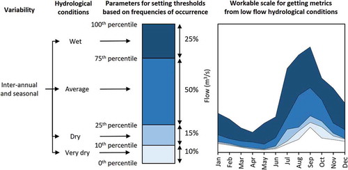
The flows characteristic of dry and very dry conditions were below the average. For these conditions, the 10^th and 0^th percentiles, respectively, set the limits. Although these conditions are outliers below the central range, they are included as an indication of dry and extremely dry historically based scenarios, which are important in highly variable regimes that regularly exhibit drought episodes likely to increase over time in many places (Reidy Liermann et al. 2012, Poff et al. 2017, Poff 2018, Arthington et al. 2018b). This is the case in two-thirds of Mexican territory – arid, semi-arid and some dry tropical climates (Méndez González et al. 2008, CONAGUA 2016). With this characterization, flows are expected to happen within the thresholds with the following natural frequency of occurrence in each hydrological condition: wet 25%, average 50%, dry 15%, and very dry 10% of the time.

3.2 High-flow pulses and flood regime

The flood regime in this method is defined as a set of peak-flow episodic events. They are identified based on the maximum daily natural or unregulated flows (m³/s) per year of the full set of records, with their corresponding magnitude, frequency, duration, time of occurrence (timing) and rate of change (rise and fall) attributes.

The set of flow events is typified for at least three categories of peaks (I, II and III) according to their historical and modelled frequencies of occurrence (recurrence intervals) at 1-, 1.5- and 5-year return periods. The recurrence intervals of these events represent the magnitude of the natural range of (I) intra-annual or high flow pulses, (II) the inter-annual characteristic of bankfull, and (III) moderate inter-annual peak events. Altogether, these events play an important role in connecting the river laterally with its floodplain and sustaining related ecological and biological processes, among other functions (Postel and Richter 2003, Richter et al. 2006 or Richter 2010).

Although peak-flow events of greater magnitude (e.g. 10- and 20-year return period) are also beneficial for the river system’s geomorphological dynamics, they are difficult to implement on site in flow-regulated cases. Generally, these rivers also face pressure on their riparian corridors and floodplains. Modeling larger events with this method are advisable only where there is neither water infrastructure – levees, water diversions and dams – along the river stream, nor human settlements – houses, towns and cities – on the river floodplain. Additionally, existing specialized studies on flooding risks must be taken into account, and the peak events characteristic of this flood regime should be supported by legal mechanisms or regulations to delimitate the public domain or space of the rivers.

The magnitude of the three categories of peak-flow events is obtained by, first, identifying the maximum daily flow per year of the full set of observed daily records considered natural or unregulated (Fig. 2(a)). Log-normal, Gumbel and log-Pearson Type III logarithmic regression models are recommended in cases where they are considered appropriate based on site-specific knowledge, such as peak-flow data symmetry/asymmetry distribution from a particular river (Chow et al. 1994). Second, the characteristic magnitude of the peak flows is selected based on the magnitude’s average associated with the 1-, 1.5- and 5-year return periods derived from the four models (the three theoretical models – log-normal, Gumbel and log-Pearson Type III, and one empirical model – historical), and the average value rounded up to a multiple of five for easy handling (Fig. 2(b)). This step is implemented for the method’s proof of concept and proposed as a standard practice. Third, the events of characteristic magnitudes are identified in the full set of observed daily records and filtered from the component of low flows (Fig. 2(c)).

Figure 2. Conceptual procedure for setting the peak-flow events based on frequencies of occurrence. (a) First, the daily maximum annual flow per year of the complete set of records is identified. (b) Second, the characteristic magnitude of the peak flows is set based on the average magnitude associated with a return period of 1, 1.5 and 5 years derived from historical, log-normal, Gumbel and log-Pearson Type-III logarithmic regression models. (c) Third, the events from characteristic magnitudes are identified in the full set of records and filtered from the low-flow component. Fourth, from this filtered set of records the characteristic duration (d) and timing (e) of the peak-flow events are identified and their cumulative frequency is calculated. Fifth, the degree of daily changes (f) is calculated for rise and fall rates

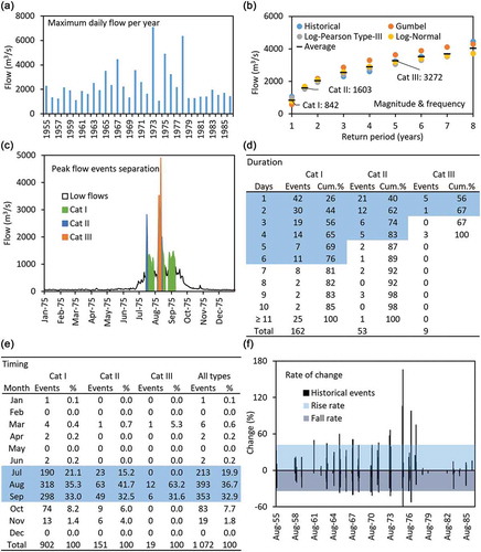
Consistent with the overall approach, the duration, timing and rate of change attributes of the peak-flow events are set upon frequency-based probability criteria, hydrologically appropriate for highly variable regimes. The duration of each episodic event (number of consecutive days that they typically last) is determined according to the cumulative relative frequency with which the flow magnitude characteristic of said events has been equalled or exceeded and, therefore, it has occurred historically in the complete natural or unregulated series of flow data. A value around 75–85% of the cumulative relative frequency of each event calculated from the complete series is adequate (Fig. 2(d)).

Likewise, the timing is determined based on the months of the natural occurrence of these same events. In the case of Mexican rivers, a relative frequency of approximately 80–90% is a functional indicator because it captures the typical seasonality of peak flow (Fig. 2(e)). With regard to the rate of change, this is set based on a percentile approach over the rise and fall of daily flow changes (%) of events that have occurred historically. The 90^th and 10^th percentiles are suitable because these parameters depict the quickest rates more closely (Fig. 2(f)).

3.3 Setting up environmental flow regimes for preventive water allocation

The criteria for setting and adjusting the eflow regimes are based on a top-down approach that places higher weight on the ecohydrological conservation merits of the flow regime over a modified condition, aligned with the preventive water allocation scope (Richter 2010, Acreman et al. 2014a, Opperman et al. 2018, Arthington et al. 2018b). The approach assumes that a river basin has different levels of water-use pressure and ecological importance, with legal eflow protection possibilities.

The criteria and process for the application of this method are described in the following sections. However, it is important to mention that the desired state or condition of an ecosystem and the future development of a river basin are the product of a societal discussion and collective agreement (Acreman et al. 2014a, 2014b, Poff et al. 2017). Furthermore, although this method can be used to diagnose the hydrological functioning of river systems, it is not appropriate for cases of over-allocated and over-exploited rivers in which the flow components need to be totally rebuilt. Examples of such cases can be seen in basins with intense consumptive usage of water that dries up the river streams for several months, and where other bottom-up, detailed approaches like habitat simulation models or holistic methodologies are more suitable.

To evaluate the hydrological integrity and assess the suitability of this methodology for implementation, we recommend the use of IHA, RVA and EFC (Richter et al. 1996, 1997, Mathews and Richter 2007). The methodology here presented is recommended for rivers whose flow records maintain their integrity under evaluation, e.g. 33 IHA parameters are within one standard deviation – i.e. ±25% around their median (25^th–75^th percentiles) – concerning the natural or reference period, for 50% of the time.

3.3.1 Environmental objectives and desired status

As reported in eflow science and practice literature (e.g. Hughes and Hannart 2003, Kendy et al. 2012, Hughes et al. 2014, Acreman et al. 2014b), a four-level environmental objective class system (A–D) was used in this method. The flow regime components and attributes are adjusted to the desired ecohydrological status. Class A means a very good state, where the flow regime keeps, or is very close to, its hydrological integrity and natural condition. Therefore, it maintains its components and their ecological-related functioning, such as wild, free-flowing or highly conserved rivers that can run through or discharge within protected areas, without disruption by anthropogenic infrastructure, such as good connectivity status (Grill et al. 2019). According to the Mexican Norm or Standard for conducting eflow assessments (NMX-AA-159-SCFI-2012; Secretaría de Economía 2012) and Salinas-Rodríguez et al. (2018), these rivers tend to have low human pressure (≤ 10% of water exploitation or stress: ratio of allocated volume for all uses divided by its availability), and high freshwater conservation values (protected species, habitats or ecosystems such as wetlands of international importance).

Classes B and C represent good and moderate desired states, respectively. Minor or sensible changes in the flow regimes of the rivers in these classes would be expected – 11–39% and 40–79% water stress, respectively – based on the Mexican case (Secretaría de Economía 2012, Salinas-Rodríguez et al. 2018). This is mostly because of the presence of small- or moderate-sized infrastructure, such as roads, levees, water diversions or dams, that have impacted the flow-related ecological integrity of the rivers. Class D represents rivers with high alteration due to moderate- to large-sized infrastructure for water use, such as hydropower or irrigation dams. Thus, the flow regime in these rivers is highly regulated; ≥80% water stress in the Mexican case (Secretaría de Economía 2012, Salinas-Rodríguez et al. 2018).

3.3.2 The frequency factors of occurrence: criteria for setting and adjusting environmental flows for water allocation

The frequency of occurrence of the hydrological conditions of low flows and the peak-flow events, presented in Tables 1 and 2, is used as a criterion for integrating eflow regimes (components and attributes) into volumes for water allocation adjusted to the desired ecohydrological status. These frequency-of-occurrence reference values were derived from the natural parameterized occurrence for each hydrological condition and the peak-flow events. They were adjusted to the four-tiered environmental objective class system based on the following reasoning supported by expert judgement and empirical knowledge (Salinas-Rodríguez et al. 2018).

Table 1. Frequency factors of occurrence for the integration of low-flow regimes into annual volumes for environmental water allocation, according to a desired ecohydrological state and environmental objective class

Desired ecohydrological status	Environmental objective	Frequency of occurrence of low-flow regimes
		Wet	Average	Dry	Very dry
Very good	A	0.1	0.4	0.3	0.2
Good	B	0.0	0.2	0.4	0.4
Moderate	C	0.0	0.0	0.4	0.6
Deficient	D	0.0	0.0	0.0	1.0

Table 2. Frequency factors of occurrence for the integration of the peak-flow events (categories I, II and III) into annual volumes for environmental water allocation, according to the desired ecohydrological state and environmental objective class

Desired ecohydrological status	Environmental objective	Frequency of occurrence of number of peak-flow events
		Category I	Category II	Category III
Very good	A	10	6	2
Good	B	5	3	2
Moderate	C	3	2	1
Deficient	D	2	1	1

A very good desired status of the low flows (environmental objective class A) and ultimately the amount of water for environmental allocation of this flow component should secure the magnitude and occurrence (frequency) in all the hydrological conditions of intra- and inter-annual variability (duration and timing) in the mid- and long term. At the same time, the eflow requirements and protection should also allow for low consumptive water usage. In this context, in a 10-year hypothetical time horizon, the wet, average, dry and very dry hydrological conditions (characteristic magnitudes and regimes) would occur with a frequency of 1, 4, 3 and 2 years, respectively, instead of 25%, 50%, 15% and 10% occurrence, as the natural frequency was characterized.

In the case of a good desired status, the proportions of the wet and average conditions decrease to zero and two years in the same 10-year horizon, respectively, while conditions dry and very dry increase to four years, as rivers within this environmental objective (Class B) generally have some water consumption rates associated with productive usage. Likewise, as long as there is more water committed to supplying productive uses, the flow regime desired status decreases and, therefore, their associated environmental objectives decline also. The frequencies of occurrence for the moderate and deficient classes of desired status (environmental objectives C and D) are proposed to follow at least the natural pattern of the flow in 4 and 6 years for dry and very dry conditions in the former case, and permanently in a very dry condition for the latter.

The algorithm to integrate the low-flow component for environmental water allocation is presented in Equation (1)(1) $Q_{\mathrm{L}\mathrm{F}}=\left(F_w\times Q_w\right)+\left(F_a\times Q_a\right)+\left(F_d\times Q_d\right)+\left(F_{vd}\times Q_{vd}\right)$(1) , which can be computed at a daily or monthly scale, and then added to obtain the annual discharge volume per hydrological condition:

(1) $Q_{\mathrm{L}\mathrm{F}}=\left(F_w\times Q_w\right)+\left(F_a\times Q_a\right)+\left(F_d\times Q_d\right)+\left(F_{vd}\times Q_{vd}\right)$(1)

where Q_LF is the annual discharge volume of low flows in hm³ (million cubic metres), F is the frequency of occurrence for the hydrological condition i (reference values in Table 1), Q is the discharge volume for the low flow i, and i is the hydrological condition for a low flow (w is wet, a is average, d is dry and vd is very dry).

For integrating the peak-flow events and considering the same hypothetical 10-year time horizon, the set of three peak-flow events (categories) would be expected to occur with their corresponding characteristic magnitudes and duration, although at different frequencies. In rivers with a very good desired ecological status and a class A environmental objective, the reference values for the frequencies are the same as the historical (natural or unregulated) ones. That is, the events of Category I (high-flow pulses) should occur at least once per year, Category II peak-flow events (inter-annual characteristic of bankfulls) would happen 6 times in 10 years, and Category III events should happen twice in 10 years (moderate inter-annual). For a good desired ecological status (Class B environmental objective) the management frequency decreases to 5/10, 3/10 and 2/10 in categories I, II and III, respectively. Similarly, for a moderate class of the desired status (environmental objective C), the frequency of occurrence decreases to 3/10, 2/10 and 1/10; and it decreases to 2/10, 1/10 and 1/10 for a deficient class (environmental objective D).

Similar to the low flows, the algorithm for integrating the peak-flow events with the flood regime component’s volume for an environmental water allocation is given in Equation (2)(2) $Q_{\mathrm{F}\mathrm{R}}=\hspace{0.17em}\frac{\left(F_{fI}\times D_{fI}\times Q_{fI}\right)+\left(F_{fII}\times D_{fII}\times Q_{fII}\right)+\left(F_{fIII}\times D_{fIII}\times Q_{fIII}\right)}{10}$(2) :

(2) $Q_{\mathrm{F}\mathrm{R}}=\hspace{0.17em}\frac{\left(F_{fI}\times D_{fI}\times Q_{fI}\right)+\left(F_{fII}\times D_{fII}\times Q_{fII}\right)+\left(F_{fIII}\times D_{fIII}\times Q_{fIII}\right)}{10}$(2)

where Q_FR is the annual discharge volume of the flood regime (hm³), F is the frequency of occurrence of the flood (f) event i (reference values in Table 2), D is the duration of the peak-flow event i, Q is the discharge volume (hm³) per day of the peak-flow event i, and i is the category of the peak-flow event (return period: I = 1, II = 1.5 or III = 5 years).

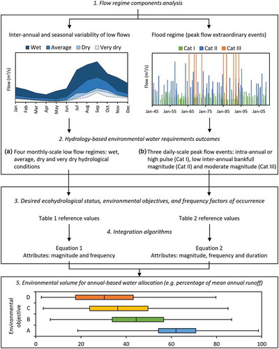
A schematic procedure of the methodology is presented in Fig. 3. The total volume for an environmental water allocation is the sum of the corresponding annual discharge (hm³) from both the low flows and the peak-flow events (flood regime). Based on the implementation of the method nationwide (up to 217 cases), by the authors of the present article and by others such as De la Lanza Espino et al. (2012, 2015), Gómez-Balandra et al. (2014), Meza-Rodríguez et al. (2017) and Hernández-Guzmán et al. (2018), the typical outcomes for environmental water allocation (median ± 25) range from 54 to 71% of the mean annual runoff (MAR) for environmental objective A, 34 to 57% for B, 24 to 50% for C and 18 to 43% for D.

Figure 3. Overall schematic procedure to determine environmental volumes for annual-based water allocation according to the hydrology-based frequency-of-occurrence approach

3.4 Case studies: application of the method and hydrological validation

The method was implemented on the San Pedro Mezquital, Baluarte and Acaponeta rivers in western Mexico (see Appendix, Section A1), all three classified with environmental objective Class A (Mexican Eflows Norm, Salinas-Rodríguez et al. 2018). The implementation followed an assessment procedure in two periods of the total observed period of flow records appropriate for this type of approach (Richter et al. 1997, Mathews and Richter 2007, Biondi et al. 2012). The objective of evaluating eflows in the case studies is to obtain recommendations for water allocation per period, to conduct a performance assessment from both sections, to examine the consistency of the outcomes and to validate the proof of concept. The two-periods-splitting approach is used to assess the degree of similarity between the metrics being evaluated, such as in a pre-impact vs post-impact assessment (e.g. Richter et al. 1996, 1997 or Mathews and Richter 2007).

Eflow recommendations are provided for consistency examination and validation. However, we recommend the use of the longest set of records possible to secure both historical and recent baselines of the flow regime. Examples of such applications of this method can be found in Alianza WWF-FGRA (2010), Sánchez Navarro and Barrios Ordóñez (2011), De la Lanza Espino et al. (2012), Hernández-Guzmán et al. (2018) or Salinas-Rodríguez et al. (2018). Furthermore, a long set of records (>40 years) is also recommended for conducting assessments with robust statistics, such as trends or novel sequences of events (King et al. 2000, Poff et al. 2017).

Daily flow records of the rivers were obtained from the national gauging stations repository operated by the Mexican National Water Commission (ftp://ftp.conagua.gob.mx/Bandas/). Each flow dataset selected for inspection had a minimum coverage of 20 consecutive years (Table 3). Furthermore, the selection was also limited to avoid gaps, inconsistencies or known impacted flows in more recent records that make their use inappropriate. This supervised inspection secured sufficient mid- to long-term representativeness of unregulated streamflow variability. The first period of record is considered a reference for validation, and the second is used for testing the approach (henceforth referred to as the assessment period).

Table 3. Flow variability indices for both the reference (earlier) and the assessment (later) periods from the case studies. MAR: mean annual runoff, CV: coefficient of variation, MABF: mean annual baseflow, BFI: baseflow index and CVB: overall index of flow variability (CV/BFI)

River basin	Gauging station (code)	Period of record	MAR (m^3/s)	CV (%)	MABF (m^3/s)	BFI (%)	CVB
San Pedro Mezquital	11012 and 11039	1944–1973	86.7	195.7	3.0	3.5	55.7
		1974–2003	86.8	275.3	1.9	2.2	123.2
Baluarte	11016	1948–1969	49.8	176.4	0.7	1.5	117.5
		1970–1992	60.3	185.4	0.8	1.3	146.5
Acaponeta	11014	1945–1976	41.6	115.8	1.6	3.9	29.9
		1977–2008	40.6	197.4	1.5	3.8	52.4

Impacted flows of the San Pedro Mezquital River (gauging station code 11012) were reconstructed due to a diversion for a relatively small-scale irrigation (~5 km upstream, station code 11039, 0.7 m³/s median annual flow, maximum peak of 1.4 m³/s in March, period 1960–2001). This reconstruction was made by adding gauged flows diverted upstream to the flow records gauged downstream on the corresponding day, and it was considered necessary for comparing the assessment period (1974–2003) against the reference period (1944–1973) under equivalent conditions, especially for the very dry low-flow condition (Alianza WWF-FGRA 2010, Sánchez Navarro and Barrios Ordóñez 2011).

The flow characteristics of the rivers exhibit an increasing seasonal variability from one record period to the other, with coefficients of variation (CV) greater than 100%, an indication that this region is subject to droughts that seriously affect both high and low flows (Hughes and Hannart 2003, Hughes et al.2014), and a potential indication of sensitivity to climate change. Alternative but less likely explanations include changes in land cover or flow management – although, based on the Mexican Eflows Norm, the human pressure on water resources in this area is low (Secretaría de Economía 2012). The San Pedro Mezquital and Acaponeta rivers both increased in variability (+41% and +70%, respectively), while the Baluarte River remained relatively stable (+5%). The three rivers initially presented perennial flow with a mean annual baseflow (MABF) from nearly 1 m³/s to 3 m³/s. The Baluarte River showed the lowest baseflow index (BFI: the ratio of MABF to MAR) of 1.3–1.5%, the lowest buffer capacity against droughts (high CV and lower BFI) and the greatest overall index of variability in both periods with values above 100 (CVB refers to the relative proportions of CV and BFI) (Hughes and Hannart 2003, Hughes et al. 2014).

The method was applied to both record periods for each river, as detailed in sections 3.1–3.3. The hydrological validation indicators were chosen based on the factors of the flow regime components that influence the outcome of Equations (1)(1) $Q_{\mathrm{L}\mathrm{F}}=\left(F_w\times Q_w\right)+\left(F_a\times Q_a\right)+\left(F_d\times Q_d\right)+\left(F_{vd}\times Q_{vd}\right)$(1) and (2(2) $Q_{\mathrm{F}\mathrm{R}}=\hspace{0.17em}\frac{\left(F_{fI}\times D_{fI}\times Q_{fI}\right)+\left(F_{fII}\times D_{fII}\times Q_{fII}\right)+\left(F_{fIII}\times D_{fIII}\times Q_{fIII}\right)}{10}$(2) ). For each hydrological condition regime, the volumes for the reference and the assessment period of the low-flow discharge per calendar month (hm³) were subtracted (residuals) and correlated. Equation (1)(1) $Q_{\mathrm{L}\mathrm{F}}=\left(F_w\times Q_w\right)+\left(F_a\times Q_a\right)+\left(F_d\times Q_d\right)+\left(F_{vd}\times Q_{vd}\right)$(1) was applied at a monthly scale for the four environmental objectives based on the frequency factors of occurrence (Table 1). The coefficients of determination (R²) and slopes were calculated according to the linear regressions of the volumes per hydrological condition, as well as for the low-flow component for environmental water allocation by such conditions and their corresponding frequencies of occurrence (using Equation 1)(1) $Q_{\mathrm{L}\mathrm{F}}=\left(F_w\times Q_w\right)+\left(F_a\times Q_a\right)+\left(F_d\times Q_d\right)+\left(F_{vd}\times Q_{vd}\right)$(1) (Fig. 4).

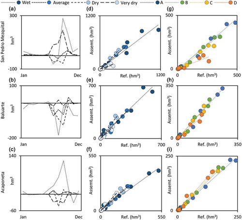
Figure 4. Reference and assessment low-flow discharge residuals (a–c), scatter plots of the low-flow hydrological conditions (d–f) and scatter plots of the integrated low flows based on the frequency factors of occurrence according to each environmental objective class (g–i)

As for the flood regime component, the flow distributions for extreme events were modelled based on the historical, log-normal, Gumbel and log-Pearson Type-III approaches (Chow et al. 1994). A total of 16 characteristic events (1-, 1.5-, 2-, 2.5-, 3-, 3.5-, 4-, 4.5-, 5-, 5.5-, 6-, 6.5-, 7-, 10-, 15- and 20-year return periods) from the four models were selected. Magnitudes associated with each recurrence interval of the characteristic event, according to the models, were averaged. R² and slope values from this new distribution were calculated and adjusted based on (i) linear regressions of the discharge magnitudes between the two sets of records and (ii) their independent logarithmic distribution models (return period vs magnitude) (Fig. 5). The magnitude (m³/s), duration and occurrence (number of consecutive days and cumulative frequency) of each peak-flow event type considered for the application of Equation (2)(2) $Q_{\mathrm{F}\mathrm{R}}=\hspace{0.17em}\frac{\left(F_{fI}\times D_{fI}\times Q_{fI}\right)+\left(F_{fII}\times D_{fII}\times Q_{fII}\right)+\left(F_{fIII}\times D_{fIII}\times Q_{fIII}\right)}{10}$(2) are displayed in supporting graphs for both the reference and the assessment periods (Figs. 6 and 7).

Figure 5. Scatter plots from characteristic magnitudes for 16 peak-flow events (floods) associated to different return periods between the reference and assessment periods (a–c), and their logarithmic distribution individual models (d–f)

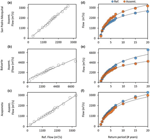
Figure 6. Daily maximum annual flow per year of the complete set of records and magnitudes of the peak-flow events of the case studies. The event magnitudes correspond to 1-, 1.5- and 5-year return periods (Categories I, II and III, respectively) for both the reference and assessment periods (left and right in each graph)

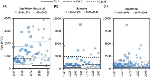
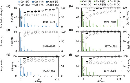
Figure 7. Number, duration (days) and cumulative frequency (percentage) of the peak-flow events of the case studies. The event magnitudes correspond to 1-, 1.5- and 5-year return periods (Categories I, II and III, respectively) from the reference (a, c and e) and assessment (b, d and f) periods

The performance assessment for each indicator was evaluated based on the R² and slope values, the first to assess the level of fitness (quality of the model) and the second to determine the level of similarity between outcomes. For the R² values, the performance indicator was assessed based on the following criteria: good > 0.9, acceptable 0.89–0.8, moderate 0.79–0.7, and low < 0.7. With regard to the slope, the performance indicator was evaluated as follows: good = 1 ± 0.1, acceptable = 1 ± 0.11–0.2, moderate = 1 ± 0.21–0.3, and low = 1 ± > 0.3. Since changes in the hydrological indicators are expected because they come from different periods, the corresponding volumes of the low flows and the flood regime of the flow regime components for environmental water allocation were examined in the context of the overall procedure and the consistency of its outcomes (validation).

4 Results

4.1 Environmental flows: regime characteristics and volumes for water allocation

Consistent with the characteristic variability of river flow (Table 3), the low flows of all the hydrological conditions experienced high variability between dry and wet seasons in the reference and assessment periods (Appendix, Table A1). During the reference period, the San Pedro Mezquital and Acaponeta rivers covered all conditions throughout the calendar months, while only wet and average conditions occurred on the Baluarte River throughout the year (with flow cessation in May in dry and very dry conditions). During the assessment period, all conditions occurred throughout the year on the Acaponeta River, while flow ceased on the Baluarte in very dry conditions (May), and in dry and very dry conditions on the San Pedro Mezquital (April–May).

River streams also showed high variability in the magnitude of their peak-flow events in the two selected periods of record (Appendix, Table A2). The comparison of the reference and the assessment periods revealed cases of major changes in the magnitude of the peak-flow events. For the high-flow pulse (Cat I), the most important changes were observed in San Pedro Mezquital, which changed from 350 to 245 m³/s (−30%) and for Baluarte, it changed from 305 to 380 m³/s (+25%). In the case of bankfulls (Cat II), Baluarte showed an increase from 800 to 995 m³/s (+24%). For the moderate inter-annual peak-flow events, San Pedro Mezquital increased as well (from 1780 to 2180 m³/s: +23%).

The peak events in all river flood categories showed a decreasing trend in the number of days (Cat I ≥ II ≥ III) and regularly lasted 1–3 days in both periods of analysis. The exception is the San Pedro Mezquital, where they lasted 2–7 days in the reference period and 1–11 days in the assessment period. Likewise, the most common timing for the peak events in all the rivers was from July to October in the reference period. However, during the assessment period, the events started to occur in June in the San Pedro Mezquital, and in January in Acaponeta and Baluarte. Concerning the rate of change, the rivers with consistency between the periods of analysis were San Pedro Mezquital (~72% ± 4 and −39%) and Baluarte (~180% and ~62% ± 6). Sensitive changes in this flow attribute were presented only for rising events in Acaponeta (from 101% to 156%).

4.2 Hydrological performance assessment and validation

In general, the greatest residuals of discharge volumes between the reference and the assessment periods were found during the wet season for all hydrological condition regimes (Fig. 4 (a)–(c)). Some notable outcomes of this indicator in the San Pedro Mezquital River occurred in July (−63 hm³) and August (−25 hm³) for the wet condition, in August for the average condition (−23 hm³), and from July to September for the dry condition (−48, −37 and −57 hm³, respectively). These changes indicate that the discharge volumes during the latter period (1974–2003) were greater than in the earlier period (1944–1973).

The Baluarte River showed a more regular discharge increase throughout the wet season between periods (1948–1969 vs 1970–1992). In this case, the mean seasonal volume residuals from June to October were −47, −29 and −53 hm³ in the wet, average and dry conditions, respectively. The Acaponeta River presented an intermediate change (1945–1976 vs 1977–2008); here the most relevant mean seasonal residuals were found in the wet and very dry conditions, with values of 50 and −16 hm³, respectively.

The variability of the river discharge residuals for all hydrological conditions was also reflected in the scatter plots of the low-flow regime outcomes from the reference and assessment periods (Fig. 4(d)–(f)). Baluarte and Acaponeta rivers showed the best overall fit in all low-flow conditions (R² ≥ 0.96; Table 4). This indicates that despite the regime differences, the outcomes of the method fit at a good quality level. However, at the slope level, the performance assessment revealed differences between periods. In the three rivers, the wet and average conditions reached at least an acceptable level of similarity (1 ± ≤ 0.2). In general, the San Pedro Mezquital also reached this level of fitness and quality, except for the very dry condition (R² = 0.84), while the slope for the dry and very dry conditions depicted higher differences [low in San Pedro and Baluarte (1 ± > 0.3), and moderate in Acaponeta (1 ± 0.21–0.3)]. Similarly, scatter plots and results of the low-flow component for environmental water allocation showed consistency within and between the four environmental objectives at a model quality level (R² = 0.96; Fig. 4(g)-(i)). Nonetheless, the slopes of their volumes depicted a lesser degree of similarity in environmental objectives C and D for San Pedro and Acaponeta, and in A, B and C for Baluarte. This is explained by the high degree of regime variability also captured between seasons (CV), the low baseflow buffer capacity (BFI) and the overall variability (CVB).

Table 4. Coefficient of determination (R²) and slope between the periods of reference and assessment for the performance validation indicators of the case study rivers

River basin	San Pedro Mezquital		Baluarte		Acaponeta
	R^2	Slope	R^2	Slope	R^2	Slope
Low flows per hydrological condition
Wet	0.95	0.86	0.96	1.11	0.99	0.80
Average	1.00	1.01	0.97	1.19	1.00	0.98
Dry	0.99	1.16	0.98	1.58	0.96	1.04
Very dry	0.84	0.43	0.96	1.02	0.99	1.23
Low flows per environmental objective
A	0.99	0.95	0.99	1.25	0.99	0.99
B	0.99	0.90	0.98	1.30	0.99	1.09
C	0.98	0.78	0.98	1.29	0.99	1.15
D	0.84	0.43	0.96	1.02	0.99	1.23
Peak flow events
Magnitude	1.00	1.27	0.96	0.64	0.99	0.92
Reference period distribution	0.99	1.08	0.96	1.12	0.99	1.11
Assessment period distribution	0.99	1.09	1.00	1.09	0.98	1.11

For the modelled characteristic flood events (Fig. 5; Table A3), the peak-flow scatter plots of the three rivers displayed a high level of fitness (R² ≥ 0.96) in both the linear regressions of the discharge magnitudes between the two sets of records and their independent logarithmic distributions (return period vs magnitude, according to each set of records). However, similar to the low-flow component, the slopes from the linear regressions depicted low to good similarities, and this is explained by the changes in magnitude of the peak-flow events from one period to the other. The logarithmic regression models exhibited acceptable to good performance.

As for the flow attributes of the peak event categories required for calculating the annual amount of water for the flood regime component (Fig. 6), the differences in magnitude are due to an increase or decrease in the maximum daily flow per year that occurred in the reference and assessment records. In San Pedro Mezquital and Baluarte they were influenced significantly (Cat I and III and Cat I and II, respectively), whereas in the Acaponeta they remained relatively constant.

In terms of differences in duration, these are related to the magnitude of the characteristic peak flows, the number of events that occurred and the set of records analysed from each period. During the reference period in the San Pedro Mezquital, 147 out of 172 total events of Cat I occurred (86% cumulative frequency) for a typical duration of 7 days, and 5/8 of Cat III (63%) with a duration of 2 days (Fig. 7(a)). In the assessment period, the typical duration changed to 11 and 1 days because there were 163/190 Cat I events (86%), and 4/6 (67%) Cat III events (Fig. 7(b)). For the Baluarte, the peak-flow duration remained practically the same (Fig. 7(c) and (d)), and in Acaponeta the difference was found in Cat II from 2 days [36/40 (90%)] to 3 days [23/26 (89%)] (Fig. 7(e) and (f)).

The annual volumes for water allocation outcomes from the two set periods of flow records is generally consistent per environmental objective. Among all cases (volumes for four environmental objectives from three rivers in two periods), in 92% the environmental volumes were < 10% MAR, and in 96% the result is within the central range of known outcomes (e.g. De la Lanza Espino et al. 2012, 2015, Gómez-Balandra et al. 2014, Meza-Rodríguez et al. 2017, Hernández-Guzmán et al. 2018, and authors’ own experience). The volumes of the low-flow component presented differences ≤ 6% MAR in the Baluarte and Acaponeta rivers, while in the San Pedro Mezquital they were 6–9% MAR in environmental objectives A–C and 17% MAR for D class (790 vs 335 hm³/year; Table A1). The volumes of the flood regime component for environmental water allocation had less than 2% difference in MAR in the three case studies for all the environmental objectives (Table A2).

5 Discussion

Since the global climate is changing because of human activities (Milly et al. 2008), the prevailing hydrological baselines in eflow assessments require more time-varying and statistical foundations to meet the non-stationarity needs (Acreman et al. 2014a, Poff et al. 2017, Arthington et al. 2018b, Poff 2018). The approach proposed here is based on wider baselines than long-term regime averages by incorporating four hydrological conditions, and the assessment is focused on two major flow regime components: low flows and a flood regime based on a set of peak-flow events.

Eflows for water allocation were calculated based on the parameterized frequency of occurrence of low flows and the set of peak-flow events. Then, as the key management factor, such flow components were adjusted to a four-level environmental objective class system. The differences between the total volume for environmental water allocation in the studied rivers were < 10% MAR in 92% of the cases for the four environmental objectives, and the volumes were largely (96%) within the central range distribution of outcomes from the previous implementation of the method.

The core assumption of this novel approach lies in the occurrence of such components. The better the desired ecohydrological state, the more natural-like the occurrence of low flows and the flood regime should be – which are key characteristics for maintaining flow–ecology relationships (Poff et al. 1997, 2017, Richter et al. 1997, Bunn and Arthington 2002, Lloyd et al. 2003, Postel and Richter 2003, Davies and Jackson 2006, Richter et al. 2006, Mathews and Richter 2007, Poff and Zimmerman 2010, Richter 2010, Stone and Menendez 2011, Acreman et al. 2014a, 2014b). Despite the short- and long-term flow variation depicted by the experimental design for the method’s proof of concept and procedure, the outcomes from its application revealed an overall good and acceptable level of fitness (model quality).

The level of fitness in the case studies explains the hydrological consistency between the total volumes for environmental water allocation for the four environmental objectives. Although differences were revealed at a slope level, these are explained by the high degree of regime variability in both periods of analysis, since changes were also depicted in the variability of the flows between seasons (CV), the baseflow buffer capacity (BFI), and the overall variability (CVB). Due to the avoidance of managed or altered flows, these outcomes suggest that such differences are inherent to regions with this level of both high- and low-flow variability, as reported by Hughes and Hannart (2003) and Hughes et al. (2014), and are a potential manifestation of climate change.

Although there are differences in the volumes of the low-flow conditions between the sets of records (i.e. the reference vs the assessment period), the validation indicator for this component exhibited a good level of fitness (R² ≥ 0.95) in the three rivers for the wet, average and dry conditions, and in two rives for the very dry condition (except San Pedro Mezquital which had an acceptable level, R² = 0.84). These levels of fitness were also presented in the low-flow component for environmental water allocation according to the management classes (R² ≥ 0.96). The only case that did not reach a good level of fitness was San Pedro’s environmental objective class D (R² = 0.84). In this river, the model fitness level was influenced by the integrated low-flow conditions, and thus depicted the sensitivity of the weight of the frequency-of-occurrence factors due to the greater (managed) frequency of very dry conditions.

As for the flood regime component, the peak-flow event indicators depicted a good level of fitness in all three rivers (R² ≥ 0.96). Similar to the low-flow component and consistent with the changes of flow variability depicted by the supporting indices (CV, BFI and CVB), the level of similarity in comparison of magnitude runs from low to good. As the corresponding in-depth magnitude analysis revealed, this is explained by the changes (increase or decrease) in the maximum daily flow per year that have occurred. Nonetheless, the logarithmic regression models exhibited slope values demonstrating acceptable to good performance. This is because the peak flows were calculated based on the average magnitude according to the recurrence interval from historical, log-normal, Gumbel and log-Pearson Type-III logarithmic regression models (Chow et al. 1994) for 16 extreme events covering a range from intra-annual high pulses to large floods (return periods from 1 to 20 years). An average-based peak-flow magnitude associated with recurrence intervals from all the distribution models holds potential as a standard practice even in cases with extremely variable regimes and thus extreme values (e.g. 10-, 15- or 20-year return period floods; Mathews and Richter 2007, Téllez Duarte et al. 2014).

From 66 validation metrics (R² and slopes) for the three indicators in the three rivers (low-flow conditions and environmental objectives, and peak-flow events) (Table 4), 83% of the cases exhibited a good and acceptable level of performance (100% R² values and 67% slopes values). The outcomes from the remaining gap, which were at a lower level, influenced the differences in the volumes for environmental water allocation. However, the results from supporting flow variability indices, as well as the in-depth analysis of flow attributes, revealed consistency, indicating that the differences were not due to the moderate or low quality of the model but because of the high degree of variability. This evidence validates the overall procedure.

Individual high- and low-flow events play short- and long-term roles in the ecosystem (Postel and Richter 2003, Richter et al. 2006, Richter 2010, Mathews and Richter 2007). They often act as important mortality agents and can shape local dynamics over shorter, management-relevant time scales (Poff et al. 2017, Poff 2018). Such events are not appropriately captured in long-term averages based on the temporal scales and prevailing foundations of hydrologic statistics; thus, they could have ecological consequences at a community level (e.g. freshwater biodiversity life strategies; Poff et al. 2017, Poff 2018). For low flows, by integrating wet, dry and very dry extreme conditions in the analysis, in addition to the average, greater variance is also incorporated. This is particularly relevant in highly variable perennial flow regimes (e.g. CV, BFI and CVB; Hughes and Hannart 2003, Hughes et al. 2014), or in intermittent rivers and ephemeral streams where the frequency and duration of (zero) low and extremely low flows are among the most important hydrological metrics (Costigan et al. 2017).

Different time-varying hydrological conditions and individual flow events can have strong effects on the performance and persistence of aquatic species (Poff et al. 2017, Poff 2018), and semi-aquatic and terrestrial species in the case of intermittent rivers and ephemeral streams (Costigan et al. 2017, Datry et al. 2017). Frequency-of-occurrence-based management for low flows and flood regime components would expose freshwater and riparian species to extreme conditions, as pointed out by Poff et al. (2017) for coping with the non-stationarity challenge, and as they naturally also occur (Poff et al. 1997, Postel and Richter 2003, Richter et al. 2006, Mathews and Richter 2007, Stone and Menendez 2011).

The assessment based on the inclusion of these conditions is supported by climatic scenarios that have occurred in the past (Poff and Matthews 2013), and event sequence trends (Poff et al. 2017) likely to occur in the future (e.g. Méndez González et al. 2008, Reidy Liermann et al. 2012, Laizé et al. 2014). It is still very difficult to predict with accuracy how extreme such conditions will get. However, by implementing eflows for wider hydrological baselines, people and nature can prepare to build their resilience based on a potential range of hydro-ecological scenarios within the ecosystem’s sustainable limits (Poff and Matthews 2013, Capon et al. 2018, Poff 2018, Arthington et al. 2018b). In water allocation systems, such eflow implementation buffers climate uncertainty due to the changing long-term regime averages (Poff 2018, Arthington et al. 2018b).

5.1 Advantages: a top-down approach for strategic environmental water allocation

The method was designed to estimate hydrology-based eflow needs, build capacities for integrating them into water management, and assist in setting standards for implementation of public policy. These motivations result from the urgent need to protect and restore aquatic ecosystems worldwide, as recently stated in the updated Brisbane Declaration and Global Action Agenda on eflows (Arthington et al. 2018a) and the Emergency Recovery Plan for bending the curve of global freshwater biodiversity loss (Tickner et al. 2020). The method follows a top-down model focused on assessing ecologically relevant flow regime components and attributes (Opperman et al. 2018). This is useful in early water management interventions for setting strategic environmental allocations in low-impact river basins with high ecological importance or freshwater conservation values, thus limiting future unsustainable water abstraction (e.g. Le Quesne et al. 2010, Richter 2010, Richter et al. 2012, Acreman et al. 2014a, 2014b, Arthington et al. 2018b, Opperman et al. 2018).

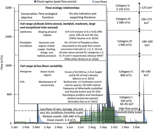
In the San Pedro Mezquital River, for example, 2297 hm³ per year (84% MAR) was allocated for environmental protection. This volume of environmental use sets the rules for water usage in the full basin in a sustainable way (SEMARNAT 2014, Salinas-Rodríguez et al. 2018). This level of protection in the context of the method implies the possibility of managing low-flow conditions that approach more closely the parameters of their natural frequency of occurrence, as well as integrating two more peak-flow events for large and exceptional magnitude floods (e.g. Cat IV = 10 and Cat V = 20-year return period). According to recent on-site studies (Blanco et al. 2011, Téllez Duarte et al. 2014, Alianza WWF-FGRA 2016, Wickel et al. 2016, Ezcurra et al. 2019), the river has molded key ecological processes in its lowland wetlands based on the current state of its flow components and attributes. Working hypotheses for supporting flow–ecology relationships, for future on-site monitoring and ecological validation, are presented in the Appendix (Section A2).

To reflect the natural occurrence of such conditions and events in San Pedro’s volume of environmental protection, adjustments in the frequency factors of occurrence needed to be made prior to the implementation of Equations (1)(1) $Q_{\mathrm{L}\mathrm{F}}=\left(F_w\times Q_w\right)+\left(F_a\times Q_a\right)+\left(F_d\times Q_d\right)+\left(F_{vd}\times Q_{vd}\right)$(1) and (2(2) $Q_{\mathrm{F}\mathrm{R}}=\hspace{0.17em}\frac{\left(F_{fI}\times D_{fI}\times Q_{fI}\right)+\left(F_{fII}\times D_{fII}\times Q_{fII}\right)+\left(F_{fIII}\times D_{fIII}\times Q_{fIII}\right)}{10}$(2) ). These consisted of factoring 0.25 wet, 0.50 average, 0.15 dry and 0.10 very dry in Table 1 instead of those values provided for class A. Likewise, large and exceptional magnitude floods with their corresponding duration (1 day) and frequency (Cat IV = 1 and Cat V = 0.5 every 10 years) should be added in Equation (2)(2) $Q_{\mathrm{F}\mathrm{R}}=\hspace{0.17em}\frac{\left(F_{fI}\times D_{fI}\times Q_{fI}\right)+\left(F_{fII}\times D_{fII}\times Q_{fII}\right)+\left(F_{fIII}\times D_{fIII}\times Q_{fIII}\right)}{10}$(2) . With these adjustments, the total volume of environmental protection would change from 2156 to 2388 hm³ (79–87% MAR). These natural frequency factors of occurrence can be considered environmental objective class A⁺ (excellent desired status of the flow regime), more appropriate for a river that discharges into a wetland of international importance (Marismas Nacionales Biosphere Reserve) with binding eflow public policy (SEMARNAT-CONANP 2013, SEMARNAT 2014).

5.2 Limitations, recommendations and future research

A factor, related to consistency of the results, to consider in further applications of the method is the quality of the flow records, which is intrinsically tied to hydrological assessments. Gaps or impaired sections in the flow records could influence outcomes. This seems to be the case in the San Pedro Mezquital performance of low flows for very dry conditions, that reached only an acceptable level. Even though the reconstruction of flow was carried out to avoid an impacted section of the records, the comparison between the reference and assessment periods revealed the sensitivity of the very dry condition parameter (0^th percentile) on the managed frequency of occurrence for the environmental objective class D.

Daily-scale, long-term observations of unregulated streamflow are recommended to reduce such sensitivity and related uncertainty, ideally for > 40 consecutive years and with < 5% gaps (King et al. 2000, Poff et al. 2017). Datasets from historical times describe well the historical regime baselines, whereas those closest to the present reflect the current ruling conditions of variability. Both are equally important and the full set of records should be, where possible, split into two, each with a sufficient range of long-term historical variability, to assess the consistency and trends between them, and to look into the novel sequences of events that may shape the ecosystem in new ways (Richter et al. 1996, 1997, King et al. 2000, Mathews and Richter 2007, Poff et al. 2017). Uncertainties in the method are likely to relate to the quality of the flow records, the appropriateness of the periods selected, and the variability caused by the inherently chaotic behaviour of the natural system (Warmink et al. 2010, Acreman et al. 2014b).

A further, important aspect is that more research is needed on the occurrence frequency factors proposed here (Tables 1 and 2) to manage the parameterized thresholds of the hydrological conditions (Fig. 1). Although this approach offers an advance in environmental water implementation, the integration criteria were formulated based on a conceptual model of decreasing water availability originally focused on highly variable flow regimes, but for perennial rivers. It is expected that such a model may be less applicable to intermittent rivers and ephemeral streams (Costigan et al. 2017). It is important to assess in detail the relative contribution of wetter and drier hydrological conditions on different river types, and their relationship over different climatic and geographic regions. The assessment of significant differences in hydrological contributions and trends in site-specific stream types, and the related socioeconomic, ecological and biological consequences, would provide new insights for adjusting the frequency-of-occurrence factors within the conceptual framework of the method. This knowledge would enrich the method and improve its outcomes in future implementation experiences as a nature-based solution in the face of a changing climate (Poff et al. 2017, Arthington et al. 2018a, 2018b, Poff 2018). It would also provide more alternatives for better adaptive management to shifts in water availability in the future for the benefit of people and ecosystems (Capon et al. 2018).

6 Conclusion

The effort developed in Mexico for protecting flows through environmental water allocation is a commitment stated in public policies at the highest level. It is based on the strategic opportunity to proactively protect flows in river basins with water availability, low demand from consumptive uses, high biological richness and conservation values.

The hydrological method presented in this article was developed and grounded in the available environmental water science and practice. It is distinguished from existing methodologies of the same kind by the use of a frequency-of-occurrence model to assess eflows and to integrate the outcomes in water allocations systems. On-site assessments play a substantial role in understanding and increasing the knowledge of ecohydrological relationships. Such knowledge is needed for monitoring, improving and validating the frequency-of-occurrence model on the ground.

The continued implementation of the method, along with in-depth studies and expanded methodologies, informs strategic decision-making for water and conservation public policies. During this process, outcomes of the method will be enriched by subsequent in-depth eflow assessments at the on-site level. This interaction will strengthen and provide the indicators for validating or adjusting the system’s legal limits for water abstraction to the sustainable level urgently needed to stop the flow alteration-related degradation of aquatic ecosystems.

Acknowledgements

We are thankful to our colleagues Hilda Escobedo and Ignacio González, and to the National Water Commission and the National Commission of Natural Protected Areas, who led the on-site implementation of San Pedro’s environmental water reserve. We also thank Nick van de Giesen and Michael McClain for their insightful feedback during the preparation of this paper, and the editors and referees.

Disclosure statement

This article is based on research conceived and developed by the authors to strengthen WWF Mexico’s Water Program from 2010 to 2019. In this paper, the authors have collectively described the method’s origins, foundations and evolution in public policies, aligned with emerging literature in environmental water science and practice. Compared to its original version (Alianza WWF-FGRA 2010, Sánchez Navarro and Barrios Ordóñez 2011), the lead author has (i) expanded the analysis to other rivers, (ii) conducted a hydrological validation assessment and (iii) quantitatively related the method’s outcomes for the San Pedro Mezquital River to recent on-site research findings for building flow–ecology relationships. The authors reported no potential conflict of interest.

Correction Statement

This article has been republished with minor changes. These changes do not impact the academic content of the article.

Additional information

Funding

The funding for the research presented in this paper was provided by the Alliance of WWF-Gonzalo Río Arronte Foundation I.A.P. (A.297), the Inter-American Development Bank (ATN/OC-12827-ME-1) and the U.S. Fish and Wildlife Service (FWS/NAWCA7F15AP00400). The submission of this article was made possible by the support of the WWF-Prince Bernhard Scholarship for Nature Conservation 2017 (Project No. 10001808/Contract No. 2583), the Mexican Council for Science and Technology (CONACYT; Reference 625567/472101) and Delft University of Technology.

Appendix

A1 Location of the case study rivers

The method was implemented on the San Pedro Mezquital, Baluarte and Acaponeta rivers in western Mexico, three of the rivers that discharge into the Marismas Nacionales (National Marshlands) region (Fig. A1). Marismas Nacionales is a protected wetland of 200 000 ha of international importance under the Ramsar Convention (Site 732), of which the Mexican government declared 133 854 ha as a biosphere reserve. The full range of variability of flows of discharging rivers is recognized by the protected area management plan for sustaining the ecological integrity, ecosystemic dynamics of the wetland, and dozens of species at risk (SEMARNAT-CONANP, 2013). At the river mouth, the official desired ecohydrological status stated in the Mexican Eflows Norm is “very good” (environmental objective class A; Secretaría de Economía 2012), and confirmed by literature review and expert knowledge for on-site assessments (Salinas-Rodríguez et al. 2018).

Table A1. Low flow volumes for water allocation per hydrological condition and environmental objective class according to Equation (1)(1) $Q_{\mathrm{L}\mathrm{F}}=\left(F_w\times Q_w\right)+\left(F_a\times Q_a\right)+\left(F_d\times Q_d\right)+\left(F_{vd}\times Q_{vd}\right)$(1) . MAR: mean annual runoff

Month	Hydrological condition (hm^3)
	Wet	Average	Dry	Very dry	Volume per environmental objective class (hm^3)
	75^th	25^th	10^th	0^th	A	B	C	D
San Pedro Mezquital
Reference period (1944–1973; MAR = 2735 hm^3/year)
January	106	23	15	9	26	14	11	9
February	53	15	11	8	16	11	9	8
March	25	10	9	7	11	9	8	7
April	12	6	5	5	6	5	5	5
May	9	5	4	3	5	4	3	3
June	106	28	11	7	27	13	9	7
July	541	324	200	183	280	218	190	183
August	831	474	323	217	413	311	259	217
September	1162	515	370	264	486	357	306	264
October	527	184	111	57	171	104	78	57
November	85	33	28	19	34	25	22	19
December	115	24	17	12	29	16	14	12
Discharge	3572	1643	1103	790	1504	1086	915	790
Assessment period (1974–2003; MAR = 2733 hm^3/year)
January	75	17	12	2	18	9	6	2
February	36	11	8	0	10	5	3	0
March	18	8	4	2	6	4	3	2
April	9	3	1	0	2	1	0	0
May	8	1	0	0	1	0	0	0
June	91	21	9	3	21	9	5	3
July	603	320	248	102	283	204	161	102
August	856	497	360	127	418	294	220	127
September	883	500	428	72	431	300	214	72
October	363	144	75	9	118	63	36	9
November	57	27	22	7	24	17	13	7
December	64	19	13	9	20	13	11	9
Discharge	3063	1569	1178	335	1354	919	672	335
Baluarte
Reference period (1948–1969; MAR = 1572 hm^3/year)
January	29	8	5	3	8	5	4	3
February	26	4	3	2	6	3	3	2
March	8	4	2	2	3	2	2	2
April	4	2	1	1	1	1	1	1
May	3	1	0	0	1	0	0	0
June	39	4	2	1	6	2	1	1
July	353	126	112	74	134	99	89	74
August	493	255	187	129	233	177	152	129
September	597	305	172	140	261	186	153	140
October	205	119	48	39	90	58	42	39
November	38	15	9	8	14	10	8	8
December	38	13	8	5	12	8	7	5
Discharge	1833	855	550	404	771	552	462	404
Assessment period (1970–1992; MAR = 1902 hm^3/year)
January	61	9	6	5	12	6	5	5
February	31	5	4	3	7	4	3	3
March	17	3	2	2	4	2	2	2
April	4	1	1	1	1	1	1	1
May	4	1	1	0	1	1	0	0
June	32	6	3	1	7	3	2	1
July	370	199	157	91	182	139	117	91
August	678	292	278	111	290	214	177	111
September	620	370	299	157	331	257	214	157
October	220	85	47	23	75	45	33	23
November	109	19	14	7	24	12	10	7
December	111	11	8	6	19	8	7	6
Discharge	2257	1001	820	406	953	690	571	406
Acaponeta
Reference period (1945–1976; MAR = 1312 hm^3/year)
January	44	8	7	5	11	7	6	5
February	17	6	5	4	6	5	4	4
March	8	5	4	3	4	4	3	3
April	6	4	3	2	4	3	3	2
May	5	4	3	2	3	3	3	2
June	42	8	5	4	10	5	4	4
July	273	134	93	39	117	80	60	39
August	437	242	178	127	220	171	148	127
September	524	250	205	144	243	190	168	144
October	167	73	43	25	64	42	32	25
November	25	13	9	8	12	9	8	8
December	35	10	9	7	11	8	7	7
Discharge	1583	756	563	370	704	524	447	370
Assessment period (1977–2008; MAR = 1281 hm^3/year)
January	34	8	6	6	10	6	6	6
February	19	6	5	4	6	4	4	4
March	10	5	4	4	5	4	4	4
April	7	3	3	2	3	3	3	2
May	5	3	3	2	3	3	2	2
June	25	7	6	3	8	5	4	3
July	242	120	78	68	109	82	72	68
August	375	246	223	150	233	198	179	150
September	402	244	188	177	230	195	181	177
October	149	63	49	20	59	40	31	20
November	56	14	9	3	14	7	5	3
December	23	10	8	6	10	8	7	6
Discharge	1347	729	581	444	690	556	499	444

Table A2. Peak flow event attributes and flood regime annual volumes for water allocation per environmental objective class according to Equation (2)(2) $Q_{\mathrm{F}\mathrm{R}}=\hspace{0.17em}\frac{\left(F_{fI}\times D_{fI}\times Q_{fI}\right)+\left(F_{fII}\times D_{fII}\times Q_{fII}\right)+\left(F_{fIII}\times D_{fIII}\times Q_{fIII}\right)}{10}$(2)

River basin	Peak event category	Reference			Assessment
		I	II	III	I	II	III
	Return period (years)	1	1.5	5	1	1.5	5
San Pedro Mezquital	Period of records	1944–1973			1974–2003
	Magnitude (m^3/s)	350	785	1780	245	845	2180
	Volume (hm^3/d)	30	68	154	21	73	188
	Duration (days)	7	3	2	11	3	1
	Timing (months)	Jul–Oct			Jun–Oct
	Rate of change (% rise and fall)	68			76
		−39			−38
	Volume per environmental objective class (hm^3/year)
	A	395			402
	B	228			220
	C	135			132
	D	93			87
Baluarte	Period of records	1948–1969			1970–1992
	Magnitude (m^3/s)	305	800	2920	380	995	2695
	Volume (hm^3/d)	26	69	252	33	86	233
	Duration (days)	3	2	1	3	2	1
	Timing (months)	Jul–Oct			Jan, Jul–Oct
	Rate of change (% rise and fall)	181			179
		−68			−55
	Volume per environmental objective class (hm^3/year)
	A	212			248
	B	131			147
	C	77			87
	D	55			60
Acaponeta	Period of records	1945–1976			1977–2008
	Magnitude (m^3/s)	215	505	1705	210	520	1500
	Volume (hm^3/d)	19	44	147	18	45	130
	Duration (days)	3	2	2	3	3	2
	Timing (months)	Jul–Oct			Jan, Jul–Oct
	Rate of change (% rise and fall)	101			156
		−62			−60
	Volume per environmental objective class (hm^3/year)
	A	167			187
	B	113			119
	C	64			69
	D	49			50

Table A3. Magnitude of the peak-flow extreme events associated with each recurrence interval (return period in years) from both the reference and assessment periods of the case study rivers

Return period	San Pedro Mezquital		Baluarte		Acaponeta
	Reference (m^3/s)	Assessment (m^3/s)	Reference (m^3/s)	Assessment (m^3/s)	Reference (m^3/s)	Assessment (m^3/s)
1.0	350	245	305	380	215	210
1.5	785	845	800	995	505	520
2.0	1050	1180	1265	1400	845	790
2.5	1270	1365	1585	1715	1045	960
3.0	1410	1535	2055	1915	1205	1090
3.5	1510	1680	2365	2150	1365	1225
4.0	1610	1890	2605	2305	1480	1350
4.5	1710	2015	2830	2510	1620	1430
5.0	1780	2180	2920	2695	1705	1500
5.5	1870	2200	3120	2775	1865	1615
6.0	1920	2340	3390	3050	1955	1770
6.5	2000	2365	3555	3130	2025	1950
7.0	2180	2615	3890	3295	2225	2015
10.0	2485	2895	4715	3830	2660	2385
15.0	2730	3250	5440	4175	3150	3035
20.0	2905	3500	7285	4705	3590	3285

A2 Flow–ecology relationships of the San Pedro River in Marismas Nacionales (basin lowlands) for on-site ecological validation

The hydrological outcomes of this method provide quantitative flow guidelines based on their historical recurrence of variability. Along with the current knowledge of environmental flow science, on-site, in-depth studies and a literature review, some flow–ecology relationships were analysed and these are proposed for future on-site monitoring and ecological validation (Fig. A2). That is, for environmental water allocation, on the one hand, the component of the low flows should secure water provisioning for at least the lower limits of each hydrological condition of the full range of the seasonal variability, at a monthly scale. On the other hand, it should secure the flood regime with a set of peak-flow extraordinary events associated with different return periods at a daily scale.

Based on the foundations of the method, the flow variability conditions of the San Pedro Mezquital River, as they occur, would also secure different longitudinal connectivity conditions. In the mid- and long term, for example, such conditions of variability should benefit and maintain the fish community. From the estuary to the river in mid-basin, the variability of the flow should allow and provide the specific requirements of movement, habitat, refuge, feeding and other seasonal needs, to secure the persistence of species populations over time (Poff 2018). These requirements should be quantitatively identified and related to the hydrological conditions, and differentiated for the life-cycle stages of the species (Richter et al. 1997, Postel and Richter 2003, Poff 2018).

According to González-Díaz et al. (2015), in the lower San Pedro Mezquital there are 11 freshwater and 41 marine species. Of those, four are currently under protection: the blackfin silverside (Atherinella crystallina), the Pacific molly (Poecilia butleri), the blackstripe livebearer (Poeciliopsis prolifica) and the lowland livebearer (Poeciliopsis latidens). All of them have a relative frequency between 15% and 40%. Key flow-related aspects require further in-depth monitoring and ecological validation of these hydrological outcomes to assess the species’ habitat and connectivity requirements for completing their life cycle (Richter et al. 2006, Mathews and Richter 2007, Acreman et al. 2014a, Acreman et al. 2014b, Poff 2018), at a river reach and regional scale.

Water depth and velocity along the river bank, and between the bank and the floodplain, are hydraulic parameters widely used to relate the flow magnitude and habitat characteristics with the fish species’ preferences and requirements for their life stages development (King et al. 2000, Poff et al. 2017). A basic working hypothesis would be that the full range of low-flow seasonal variability sustains these fish community baselines. Based on the outcomes of the methods used here, the mean flow range recommendations would be 1–24 m³/s for dry season (November–June; 1–3 m³/s in May as the driest month) and 30–290 m³/s for wet season (July–October; 100–440 m³/s in September as the wettest month). Other more challenging hypotheses would be that in the mid- to long term, considering the four hydrological conditions, these fish baselines should be maintained according to the ranges of mean dry-season low flows of 17–24 m³/s for wet condition, 5–7 m³/s average, 3–5 m³/s dry and 1–3 m³/s very dry (3 ± 0.1 m³/s, 1.1 ± 0.7 m³/s, 0.8 ± 0.7 m³/s and 0.5 ± 0.5 m³/s, respectively, in May). Likewise, the mean wet-season low flows would be 255–290 m³/s for wet condition, 138–141 m³/s average, 95–105 m³/s dry, and 29–68 m³/s very dry (395 ± 50 m³/s, 196 ± 3 m³/s, 155 ± 10 m³/s and 65 ± 35 m³/s, respectively, in September).

Similarly, the freshwater discharge would maintain its exchange with the marine water, as well as the salinity gradient based on the conditions of the low-flows regimes (King et al. 2000, Marchand 2003). Over time, these regimes have contributed to this brackish environment favourable for the establishment of the mangrove forest, with a reported extension within the influence of San Pedro of nearly 63 600 ha, from 2 to 8 m height and a tree density of 8–55 (Blanco et al. 2011). In this case, a flow-related aspect to monitor would be the salinity gradient along the river and in the estuary, and its relation with the freshwater discharge, the forest structure and the mangrove species composition. The working hypothesis for the ecological validation would be that the full range of low flows derived from this approach sustains the mangrove structure and species composition, with the salinity gradient and the freshwater discharge as quantitative indicators.

The flood regime and its full set of peak-flow event components should guarantee the lateral connectivity of the San Pedro River (Mathews and Richter 2007, Acreman et al. 2014a). The interaction between the river and its floodplain provides ecological functions such as triggering migration spawning cues for fish and new life phases in aquatic invertebrates, and providing new habitats, flush organic matter and woody debris, among other things (Postel and Richter 2003, Richter et al. 2006, Poff 2018). Recent in-depth studies in the lower San Pedro have identified flow-related quantitative indicators for keeping the hydrogeomorphological processes and linkages between the river discharge and its delta.

Téllez Duarte et al. (2014) studied the influence of San Pedro on sediment deposition and texture at the river delta. They found that over the last 40 years the river has deposited a cumulative rate of sediments at an average range of 0.9–3.9 (±0.1–0.6) centimetres per year, with 64%, 33% and 3% of sand, silt and clay proportions, respectively. The intra-annual, bankfull and moderate magnitude peak-flow events of the river (1-, 1.5- and 5-year return period) longitudinally transport these sediment loads. However, large and exceptional floods (10- and 20-year return periods) play a greater role in dispersing them over the floodplain for the additional exchange of water, nutrients and organic matter.

Furthermore, and based on a recent remote sensing analysis on the coastal floodplain wetlands of the San Pedro River (Wickel et al. 2016), the flooded surface extension influenced by the full set of peak-flow events ranges from approximately 65 km² to more than 175 km². This area of periodic lateral connectivity represents feeding, refuge and habitat provision opportunities for fish in the wet season, and for resident and winter-season migratory waterfowl (Alianza WWF-FGRA 2016). In this case, the working hypothesis would be that the peak-flow events, particularly the characteristic bankfull, moderate inter-annual, large and exceptional ones, carry the sediment volumes for sustaining the cumulative deposition rates and particle texture, as reported in this geomorphologic dynamic (Téllez Duarte et al. 2014). Based on the two record periods, the recommended flow magnitudes would be around 350 m³/s (Cat I), 800 m³/s (Cat II), 1900 m³/s (Cat III), 2580 m³/s (Cat IV) and 3110 m³/s (Cat V). Another opportunity for better understanding the ecological relevance of this regime component would be to track the flooding extent surface via periodic remote sensing analysis (e.g. every 3–5 years), as well as validating the beneficial aspects through the needs of fish and birds.

Figure A1. Location of the San Pedro Mezquital, Baluarte and Acaponeta rivers

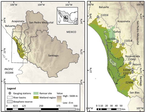
Figure A2. Flow–ecology relationships of the San Pedro River in Marismas Nacionales (basin lowlands). The conceptual hydrograph is shown at two time scales: daily, for differentiating the peak-flow events of the flood regime (dark blue; categories in dashed lines) from low flows (light blue); and monthly, for the low-flow regime thresholds (light green and solid lines)

References

- Acreman, M.C., et al., 2014a. Environmental flows for natural, hybrid, and novel riverine ecosystems in a changing world. Frontiers in Ecology and the Environment, 12 (8), 466–473. doi:10.1890/130134
- Acreman, M.C., et al., 2014b. The changing role of ecohydrological science in guiding environmental flows. Hydrological Sciences Journal, 59 (3–4), 433–450. doi:10.1080/02626667.2014.886019
- Alianza WWF-Fundación Gonzalo Río Arronte I.A.P. (FGRA), 2010. Propuesta de caudal ecológico en la cuenca San Pedro en Marismas Nacionales y su consideración en el estudio de disponibilidad de aguas superficiales. Mexico: WWF, Reporte técnico del Programa Agua.
- Alianza WWF-Fundación Gonzalo Río Arronte I.A.P. (FGRA), 2016. Reserva ambiental de agua: asegurando el habitat de aves migratorias. Mexico: WWF, Reporte final técnico y financiero (No. de grant FSW/NAWCA7F15AP00400).
- Alonso-Eguía Lis, P.E., Gómez-Balandra, M.A., and Saldaña-Fabela, P., eds, 2007. Requerimientos para implementar el caudal ambiental en México. Jiutepec, Morelos, Mexico: IMTA-Alianza WWF/FGRA-PHI/UNESCO-SEMARNAT.
- Arthington, A.H., et al., 2018a. The Brisbane Declaration and global action agenda on environmental flows (2018). Frontiers in Environmental Science, 6 (45), 1–15. doi:10.3389/fenvs.2018.00045
- Arthington, A.H., et al., 2018b. Recent advances in environmental flows science and water management–Innovation in the Anthropocene. Freshwater Biology, 63 (8), 1022–1034. doi:10.1111/fwb.13108
- Barrios-Ordóñez, J.E., et al., 2015. National Water Reserves Program in Mexico. Experiences with environmental flows and the allocation of water for the environment. M.E. De la Peña, G. Ramírez and C. Alcalá, eds. Mexico: Inter-American Development Bank, Water and Sanitation Division, Technical Note No. BID-TN-864.
- Biondi, D., et al., 2012. Validation of hydrological models: conceptual basis, methodological approaches and a proposal for a code of practice. Physics and Chemistry of the Earth, 42–44, 70–76. doi:10.1016/j.pce.2011.07.037
- Blanco, M., et al., ed, 2011. Diagnóstico funcional de Marismas Nacionales. Tepic, Nayarit, Mexico: Universidad Autónoma de Nayarit, Comisión Nacional Forestal y Gobierno del Reino Unido, Informe final de los convenios de coordinación.
- Bunn, S.E. and Arthington, A.H., 2002. Basic principles and ecological consequences of altered flow regimes for aquatic biodiversity. Environmental Management, 30 (4), 492–507. doi:10.1007/s00267-002-2737-0
- Capon, S.J., et al., 2018. Transforming environmental water management to adapt to a changing climate. Frontiers in Environmental Science, 6 (80), 1–10. doi:10.3389/fenvs.2018.00080
- Chow, V.T., Maidment, D.R., and Mays, L.W., 1994. Hidrología aplicada. Colombia: McGraw-Hill Interamericana S.A. de C.V.
- Comisión Nacional del Agua (CONAGUA), 2016. Estadísticas del agua en México, edición 2016. Mexico City, Mexico: Secretaría de Medio Ambiente y Recursos Naturales.
- Comisión Nacional del Agua (CONAGUA), 2020. Programa Nacional Hídrico 2020–2024 Resumen. Mexico City, Mexico: Secretaría de Medio Ambiente y Recursos Naturales.
- Costigan, K.H., et al., 2017. Flow regimes in intermittent rivers and ephemeral streams, in Intermittent rivers and ephemeral streams. In: T. Datry, N. Bonada, and A. Boulton, eds. Ecology and management. London, UK: Academic Press, 51–78.
- Datry, T., Bonada, N., and Boulton, A., eds., 2017. Intermittent rivers and ephemeral streams. Ecology and management. London, UK: Academic Press.
- Davies, S.P. and Jackson, S.K., 2006. The biological condition gradient: A descriptive model for interpreting change in aquatic ecosystems. Ecological Applications, 16 (4), 1251–1266. doi:10.1890/1051-0761(2006)016
- De la Lanza Espino, G., et al., 2012. Measurement of the ecological flow of the Acaponeta River, Nayarit, comparing different time intervals. Investigaciones Geográficas, Boletín del Instituto de Geografía (In Spanish), UNAM, 78, 62–74. doi:10.14350/rig.32470
- De la Lanza Espino, G., Salinas Rodríguez, S.A., and Carbajal López, J.L., 2015. Environmental flow calculation for the maintenance of the water reserve of the Piaxtla River, Sinaloa, Mexico. Investigaciones Geográficas, Boletín del Instituto de Geografía (In Spanish), UNAM, 87, 62–74. doi:10.14350/rig.35269
- Dudgeon, D., et al., 2006. Freshwater biodiversity: importance, threats, status and conservation challenges. Biological Reviews, 81 (2), 163–182. doi:10.1017/S1464793105006950
- Ezcurra, E., et al., 2019. A natural experiment reveals the impact of hydroelectric dams on the estuaries of tropical rivers. Science Advances, 5 (3), eaau9875. doi:10.1126/sciadv.aau9875
- García, E., et al., 1999. Guía de aplicacipón de los métodos de cálculo de caudales de reserva ecológicos en México. Mexico: CAN-IMTA-SEMARNAP.
- Gómez-Balandra, M.A., Saldaña-Fabela, M.P., and Martínez-Jiménez, M., 2014. The Mexican environmental flow standard: scope, application and implementation. Journal of Environmental Protection, 5, 71–79. doi:10.4236/jep.2014.51010
- González-Díaz, A.Á., et al., 2015. Fishes in the lower San Pedro Mezquital River, Nayarit, Mexico. Check List, 11 (6), 1797. doi:10.15560/11.6.1797
- Grill, G., et al., 2019. Mapping the world’s free-flowing rivers. Nature, 569, 215–221. doi:10.1038/s41586-019-1111-9
- Harwood, A., et al., 2017. Listen to the river: lessons from a global review of environmental flow success stories. Woking, UK: WWF-UK.
- Hernández-Guzmán, R., Ruiz-Luna, A., and Cervantes-Escobar, A., 2018. Environmental flow assessment for rivers feeding a coastal wetland complex in the Pacific coast of northwest Mexico. Water and Environment Journal, 1–11. doi:10.1111/wej.12423
- Horne, A.C., O’Donnell, E.L., and Tharme, R.E., 2017. Mechanisms to allocate environmental water. In: A.C. Horne, et al., eds. Water for the environment. From policy and science to implementation and management. San Diego, CA: Academic Press, 361–398.
- Hughes, D.A., et al., 2014. A new approach to rapid, desktop-level, environmental flow assessments for rivers in South Africa. Hydrological Sciences Journal, 59 (3–4), 673–687. doi:10.1080/02626667.2013.818220
- Hughes, D.A. and Hannart, P., 2003. A desktop model used to provide an initial estimate of the ecological instream flow requirements of rivers in South Africa. Journal of Hydrology, 270 (3–4), 167–181. doi:10.1016/S0022-1694(02)00290-1
- Kendy, E., Apse, C., and Blann, K., 2012. A practical guide to environmental flows for policy and planning, with nine case studies from the United States [online]. The Nature Conservancy. Available from: https://www.conservationgateway.org/ConservationPractices/Freshwater/EnvironmentalFlows/MethodsandTools/ELOHA/Documents/Practical%20Guide%20Eflows%20for%20Policy-low%20res.pdf [Accessed 28 July 2017].
- King, J.M., Tharme, R., and de Villiers, M.S., 2000. Environmental flow assessments for rivers: manual for the Building Block Methodology. Freshwater Research Unit, University of Cape Town, South Africa: Water Research Commission Report No. TT 131/00.
- Laizé, C.L.R., et al., 2014. Projected flow alteration and ecological risk for Pan-European rivers. River Research and Applications, 30 (3), 299–314. doi:10.1002/rra.2645
- Le Quesne, T., Kendy, E., and Weston, D., 2010. The implementation challenge – taking stock of government policies to protect and restore environmental flows. Surrey, UK: World Wildlife Fund and The Nature Conservancy.
- Lloyd, N., et al., 2003. Does flow modification cause geomorphological and ecological response in rivers? A literature review from an Australian perspective. Canberra, Australia: Cooperative Research Centre for Freshwater Ecology, Technical Report 1/2004.
- Marchand, M., 2003. Environmental flow requirements for river. An integrated approach for river and coastal zone management. Delft, The Netherlands: WL|Delft Hydraulics, Integrated Water Management/Water Systems (ENFRAIM), Final project report code 06. 02.04.
- Mathews, R. and Richter, B.D., 2007. Application of the indicators of hydrologic alteration software in environmental flow setting. Journal of the American Water Resources Association, 43 (6), 1400–1413. doi:10.1111/j.1752-1688.2007.00099.x
- Mekonnen, M.M. and Hoekstra, A.Y., 2016. Four billion people facing severe water scarcity. Science Advances, 2 (2), e150032. doi:10.1126/sciadv.1500323
- Méndez González, J., Návar Cháidez, J.J., and González Ontiveros, V., 2008. Analysis of rainfall trends (1920–2004) in Mexico. Investigaciones Geográficas, Boletín Del Instituto De Geografía (In Spanish), UNAM, 65, 38–55.
- Meza-Rodríguez, D., et al., 2017. Propuesta de caudal ecológico en la cuenca del Río Ayuquila-Armería en el Occidente de México. Latin American Journal of Aquatic Research, 45 (5), 1017–1030.
- Milly, P.C.D., et al., 2008. Stationarity is dead: whither water management? Science, 319 (5863), 573–574. doi:10.1126/science.1151915
- Moir, K., Thieme, M., and Opperman, J., 2016. Securing a future that flows: case studies of protection mechanisms for rivers. Washington, DC: World Wildlife Fund and The Nature Conservancy.
- Opperman, J.J., et al., 2018. A three-level framework for assessing and implementing environmental flows. Frontiers in Environmental Science, 6 (76), 1–13. doi:10.3389/fenvs.2018.00076
- Organisation for Economic Co-operation and Development (OECD), 2012. OECD environmental outlook to 2050. OECD Publishing. doi:10.1787/9789264122246-en
- Petts, G.E., 2009. Instream flow science for sustainable river management. Journal of the American Water Resources Association, 45 (5), 1071–1086. doi:10.1111/j.1752-1688.2009.00360.x
- Poff, N.L., et al., 1997. The natural flow regime: a new paradigm for riverine conservation and restoration. BioScience, 47 (11), 769–784. doi:10.2307/1313099
- Poff, N.L., 2018. Beyond the natural flow regime? Broadening the hydro-ecological foundation to meet environmental flow challenges in a non-stationary world. Freshwater Biology, 63 (8), 1011–1021. doi:10.1111/fwb.13038
- Poff, N.L. and Matthews, J.H., 2013. Environmental flows in the Anthropocence: past progress and future prospects. Current Opinion in Environmental Sustainability, 5 (6), 667–675. doi:10.1016/j.cosust.2013.11.006
- Poff, N.L., Tharme, R.E., and Arthington, A.H., 2017. Evolution of environmental flow assessments science, principles, and methodologies. In: A.C. Horne, et al., eds. Water for the environment. From policy and science to implementation and management. San Diego, CA: Academic Press, 203–236.
- Poff, N.L. and Zimmerman, J.K.H., 2010. Ecological responses to altered flow regimes: a literature review to inform the science and management of environmental flows. Freshwater Biology, 55 (1), 194–205. doi:10.1111/j.1365-2427.2009.02272.x
- Postel, S. and Richter, B., 2003. Rivers for life. Managing water for people and nature. USA: Island Press.
- Reidy Liermann, C.A., et al., 2012. Hydrogeomorphic classification of Washington state rivers to support emerging environmental flow management strategies. River Research and Applications, 28 (9), 1340–1358. doi:10.1002/rra.1541
- Richter, B.D., et al., 1996. A method for assessing hydrologic alteration within ecosystems. Conservation Biology, 10 (4), 1163–1174. doi:10.1046/j.1523-1739.1996.10041163.x
- Richter, B.D., et al., 1997. How much water does a river need? Freshwater Biology, 37 (1), 231–249. doi:10.1046/j.1365-2427.1997.00153.x
- Richter, B.D., et al., 2006. A collaborative and adaptive process for developing environmental flow recommendations. River Research and Applications, 22 (3), 297–318. doi:10.1002/rra.892
- Richter, B.D., 2010. Re-thinking environmental flows: from allocations and reserves to sustainability boundaries. River Research and Applications, 26 (8), 1052–1063. doi:10.1002/rra.1320
- Richter, B.D., et al., 2012. A presumptive standard for environmental flow protection. River Research and Applications, 28 (8), 1312–1321. doi:10.1002/rra.1511
- Salinas-Rodríguez, S.A., et al., 2018. Environmental flows and water reserves: principles, strategies, and contributions to water and conservation policies in Mexico. River Research & Applications, 34 (8), 1057–1084. doi:10.1002/rra.3334
- Sánchez Navarro, R. and Barrios Ordóñez, E., 2011. Caudal ecológico: propuesta metodológica. Ejemplo de caso río San Pedro Mezquital, Marismas Nacionales, Nayarit. In: G. De la Lanza Espino and S. Hernández, eds. Ambiente, biología, sociedad, manejo y legislación de sistemas coteros mexicanos. Mexico City, Mexico: Plaza y Valdés S.A. de C.V., 437–469.
- Santacruz de León, G. and Aguilar-Robledo, M., 2009. Estimates of ecological flows in the Río Valles with the Tennant method. Hidrobiológica, 19 (1), 25–32.
- Secretaría de Economía, 2012. NMX-AA-159-SCFI-2012 that establishes the procedure for environmental flow determination in hydrological basins. Mexico: Diario Oficial de la Federación (20/09/2012).
- Secretaría de Gobernación (SEGOB), 2013. Programa sectorial de medio ambiente y recursos naturales 2013–2018. Mexico: Diario Oficial de la Federación (12/12/2013).
- Secretaría de Gobernación (SEGOB), 2014a. Programa nacional hídrico 2014–2018. Mexico: Diario Oficial de la Federación (08/04/2014).
- Secretaría de Gobernación (SEGOB), 2014b. Programa especial de cambio climático 2014–2018. Mexico: Diario Oficial de la Federación (28/04/2014).
- Secretaría de Medio Ambiente y Recursos Naturales (SEMARNAT), 2014. Decreto por el que se abrogan los acuerdos que se indican y se establece la reserva de aguas en las cuencas que se señala. Mexico: Diario Oficial de la Federación (15/09/2014).
- Secretaría de Medio Ambiente y Recursos Naturales and Comisión Nacional de Áreas Naturales Protegidas (SEMARNAT-CONANP), 2013. Programa de manejo: reserva de la biósfera Marismas Nacionales. Mexico: Secretaría de Medio Ambiente y Recursos Naturales.
- Smakhtin, V.U. and Eriyagama, N., 2008. Developing a software package for global desktop assessment of environmental flows. Environmental Modelling and Software, 23 (12), 1396–1406. doi:10.1016/j.envsoft.2008.04.002
- Stone, E. and Menendez, L., 2011. Natural disturbance regime [online]. In: J. Cutler, M. McGinley, and C.J. Cleveland, eds. Encyclopedia of Earth. Available from: https://editors.eol.org/eoearth/wiki/Natural_disturbance_regime [Accessed 8 January 2017].
- Téllez Duarte, M.A., et al., 2014. Ambientes y procesos hidrosedimentarios en la cuenca hidrográfica del río San Pedro Mezquital en Marismas Nacionales. Mexico: CONAGUA-BID-Alianza World Wildlife Fund-Fundación Gonzalo Río Arronte, Informe final de los convenios de coordinación ON94 BID y OP26 Alianza WWF-FGRA.
- Tennant, D.L., 1976. Instream flow regimes for fish, wildlife, recreation and related environmental resources. Fisheries, 1 (4), 6–10. doi:10.1577/1548-8446(1976)001<0006:IFRFFW>2.0.CO;2
- Tharme, R.E., 2003. A global perspective on environmental flows assessment: emerging trends in the development and application of environmental flow methodologies for rivers. River Research and Applications, 19 (5–6), 397–441. doi:10.1002/rra.736
- Tickner, D., et al., 2020. Bending the curve of global freshwater biodiversity loss: an emergency recovery plan. BioScience, 1–13. doi:10.1093/biosci/biaa002
- Warmink, J.J., et al., 2010. Identification and classification of uncertainties in the application of environmental models. Environmental Modelling & Software, 25 (12), 1518–1527. doi:10.1016/j.envsoft.2010.04.011
- Wickel, A.J., et al., 2016. Environmental water reserves: securing water for migratory waterbird habitat. USA: Stockholm Environment Institute, World Wildlife Fund-Fundación Gonzalo Río Arronte, Comisión Nacional para el Conocimiento y Uso de la Biodiversidad, and U.S. Fish & Wildlife Service, Technical report on Agreement OR78 FWS, Division of Bird Habitat & Conservation.
- WWF, 2018. Living planet report - 2018: aiming higher. Grooten, M. and R.E.A., Almond, eds. Switzerland: WWF.
- Yarnell, S.M., et al., 2015. Functional flows in modified riverscapes: hydrographs, habitats and opportunities. BioScience, 65, 963–972. doi:10.1093/biosci/biv102