New approach to computing mean velocity and discharge

ABSTRACT

Estimation of discharge hydrograph may be needed at river gauging stations where discharge is computed by converting water stage using a stage-discharge relation (a rating curve) or multiplying mean velocity by flow cross-sectional area. The mean velocity is computed by converting the measured maximum velocity to mean velocity using a conversion factor. Estimating the velocity conversion factor at stations where measured discharge data are insufficient remains a challenge. This study develops a novel method for determining the conversion factor by combining the entropy velocity profile, a data-driven technique, and a one-dimensional (1-D) flood routing model, and thus develops a method to determine discharge at the weak gauging sites. The method was used with two different assumptions: constant velocity factor and velocity factor depending on the aspect ratio. Results showed that this method optimally estimated the conversion factor.

KEYWORDS:

• entropy velocity profile
• roughness
• width to water depth ratio
• mean velocity
• water discharge

Editor A. Castellarin Associate editor A. Domeneghetti

Introduction

Evaluation of water discharge in open channels is required in irrigation, river monitoring and control, water resources management, water balance assessment at the basin scale, design of hydraulic structures, and calibration and validation of runoff and flood routing models (Greco 2016). Measurement of discharge at gauging stations requires information about the mean velocity in a number of subsections across the channel and their cross-section geometry. Flow velocity measurements are carried out by current meters across the channel in order to calculate the total stream discharge. Discharge values are used to define the cross-section rating curve, which is an essential operative tool for river flow management even during floods. In rivers, the velocity distribution is affected by channel geometry, vegetation and roughness. In wide channels flow velocity increases monotonically from 0 at the channel bed to the maximum value near or below the water surface, and the velocity distribution may be considered one-dimensional (1-D) (Greco 2015). In narrow channels, the velocity is influenced by the boundaries and varies even along the transverse direction, and the velocity distribution may become predominantly two-dimensional. The maximum velocity may occur at or below the water surface, inducing dip-phenomena, and the position of maximum velocity is influenced by the aspect ratio (B/D), where B is the channel width and D is the water depth (Ferro 2003, Yang et al. 2004, Moramarco et al. 2017). Recently, several studies have estimated mean velocity by applying entropy. Using Shannon entropy, Chiu (1987) introduced a relation between the ratio of mean to maximum velocity (u_m and u_max, respectively) and entropy (M) as:

(1) ${\mathrm{\Phi }}_M=\frac{u_m}{u_{\mathrm{m}\mathrm{a}\mathrm{x}}}=\frac{e^M}{e^M-1}-\frac{1}{M}$(1)

Several authors have investigated the accuracy of this relationship using field data (Xia 1997, Moramarco et al. 2004, Farina et al. 2014, Greco et al. 2014, Greco and Mirauda 2015) and found ${\mathrm{\Phi }}_M$ and, hence, M to be constant at a river site and unaffected by the magnitudes of floods. Moramarco and Singh (2010) investigated the dependence of M on hydraulic and geometric characteristics at a river site and showed that M was not dependent on the dynamics of flood, because it did not depend on the energy or the water surface slope, S_f. Hence, the formula expressing M as a function of hydraulic radius, Manning’s roughness coefficient and elevation, y₀, where the horizontal velocity is hypothetically equal to zero, was identified. Since y₀ is not simple to assess and would be subject to uncertainty, the assessment of M should be addressed using hydraulic and geometric variables that are easy to measure mainly for ungauged river sites. During high floods, the measurement of velocity is possible only in the upper portion of the flow area where the maximum velocity occurs. In this way, the knowledge of M, and hence of the entropic relationship, Equation (1)(1) ${\mathrm{\Phi }}_M=\frac{u_m}{u_{\mathrm{m}\mathrm{a}\mathrm{x}}}=\frac{e^M}{e^M-1}-\frac{1}{M}$(1) , can be useful for computing mean velocity. It is noted that the estimation of M is easy if there is a robust velocity dataset containing the pairs (u_m, u_max). The dependence of M on the water depth and roughness height is more evident in shallow-water conditions where M can be influenced by roughness height, but in high-flow conditions it is found to be constant (Bathurst et al. 1981, Bathurst 1985, Moramarco and Singh 2010). Using the entropy-based velocity profile law and classical relationships for uniform flow and friction factor, Greco (2015) proposed a general logarithmic relationship between parameter Φ_M, Equation (1)(1) ${\mathrm{\Phi }}_M=\frac{u_m}{u_{\mathrm{m}\mathrm{a}\mathrm{x}}}=\frac{e^M}{e^M-1}-\frac{1}{M}$(1) , and the ratio of water depth to bed roughness (D/d). Greco and Moramarco (2015) introduced a similar relationship between ${\mathrm{\Phi }}_M$ and the ratio between water width, B, and flow depth, D:

(2) ${\mathrm{\Phi }}_M=A_B\mathrm{I}\mathrm{n}\frac{B}{D}+C_B$(2)

where A_B and C_B are the appropriate coefficients. Using Equation (2)(2) ${\mathrm{\Phi }}_M=A_B\mathrm{I}\mathrm{n}\frac{B}{D}+C_B$(2) , one can easily estimate Φ_M by measuring only channel width and flow depth, and hence, through Equation (1)(1) ${\mathrm{\Phi }}_M=\frac{u_m}{u_{\mathrm{m}\mathrm{a}\mathrm{x}}}=\frac{e^M}{e^M-1}-\frac{1}{M}$(1) the mean velocity and discharge can be inferred. Therefore, it is of considerable interest to estimate parameters A_B and C_B at river sites where velocity data are not available.

In this context, this study proposes a simple method for estimating parameters in Equation (2)(2) ${\mathrm{\Phi }}_M=A_B\mathrm{I}\mathrm{n}\frac{B}{D}+C_B$(2) at ungauged river sites. The method is also extended to the case of ${\mathrm{\Phi }}_M$constant as expressed by Equation (1)(1) ${\mathrm{\Phi }}_M=\frac{u_m}{u_{\mathrm{m}\mathrm{a}\mathrm{x}}}=\frac{e^M}{e^M-1}-\frac{1}{M}$(1) , and results on discharge assessment are compared with those of Equation (2)(2) ${\mathrm{\Phi }}_M=A_B\mathrm{I}\mathrm{n}\frac{B}{D}+C_B$(2) . The proposed method was tested using data from the Ponte Nuovo station on the Tiber River, Italy.

Brief theoretical background on the entropy parameter M

For a gauged site where a dataset of pairs (u_m, u_max) is available, M can be easily estimated. For ungauged sites, Greco (2015) derived an equation between velocity ratio and water depth to roughness height ratio by combining hydraulic relations and the entropy-based velocity profile equation:

(3) ${\mathrm{\Phi }}_M=\frac{U_m}{U_{max}}=A_{\mathrm{\Phi }}\mathrm{I}\mathrm{n}\frac{D}{d}+B_{\mathrm{\Phi }}$(3)

where A_Φ and B_Φ are the numerical coefficients, D is the maximum water depth, and d is the characteristic dimension of roughness elements. Equation (3)(3) ${\mathrm{\Phi }}_M=\frac{U_m}{U_{max}}=A_{\mathrm{\Phi }}\mathrm{I}\mathrm{n}\frac{D}{d}+B_{\mathrm{\Phi }}$(3) reflects the possible effect of bed roughness on the entropy-based velocity distribution in open-channel flow, depending on the scale of large, intermediate and small roughness elements. Studies have shown that it is possible to express average flow width (B) and depth, as well as the ratio D/d, as functions of water discharge (Q) (Leopold and Maddock 1953, Leopold et al. 1964, Griffiths 1980):

(4) $\left\{\begin{array}{c}B=\alpha Q^a\\ D=\beta Q^b\\ \frac{D}{d}=\frac{\gamma }{i{\mathrm{\%}}^j}{Q}^c\end{array}\right.$(4)

in which i% represents the local bed slope, and a, b, c, α, β, γ and j are the numerical coefficients. After a little algebra, the relative submergence can be reported in terms of the aspect ratio, B/D, obtaining the following (Greco and Moramarco 2015):

(5) $\frac{D}{d}=\frac{\gamma }{i{\mathrm{\%}}^j}{\left[\frac{\beta }{\alpha }.\frac{B}{D}\right]}^{\frac{c}{\alpha -b}}=K^{\ast }{\left(\frac{B}{D}\right)}^{{\alpha }^{\ast }}$(5)

where k* and a* are the coefficients. Finally, Equation (3)(3) ${\mathrm{\Phi }}_M=\frac{U_m}{U_{max}}=A_{\mathrm{\Phi }}\mathrm{I}\mathrm{n}\frac{D}{d}+B_{\mathrm{\Phi }}$(3) can be reformulated taking into account Equation (5)(5) $\frac{D}{d}=\frac{\gamma }{i{\mathrm{\%}}^j}{\left[\frac{\beta }{\alpha }.\frac{B}{D}\right]}^{\frac{c}{\alpha -b}}=K^{\ast }{\left(\frac{B}{D}\right)}^{{\alpha }^{\ast }}$(5) , and the velocity ratio Φ_M can be derived as a function of B/D as expressed by Equation (2)(2) ${\mathrm{\Phi }}_M=A_B\mathrm{I}\mathrm{n}\frac{B}{D}+C_B$(2) .

Equation (2)(2) ${\mathrm{\Phi }}_M=A_B\mathrm{I}\mathrm{n}\frac{B}{D}+C_B$(2) can be useful in the mean velocity and discharge estimation, especially in high-flow conditions, because if the channel section, water depth and water width are known and by using proper coefficients, A_B, C_B in Equation (2)(2) ${\mathrm{\Phi }}_M=A_B\mathrm{I}\mathrm{n}\frac{B}{D}+C_B$(2) , Φ_M can be estimated and then the mean velocity if u_max is measured. In this study, a methodology to estimate coefficients A_B and C_B at stations without adequate data, using a combination of Equation (2)(2) ${\mathrm{\Phi }}_M=A_B\mathrm{I}\mathrm{n}\frac{B}{D}+C_B$(2) and hydraulic modelling (HEC-RAS) with one data-driven technique, is introduced.

Hydraulic modelling (HEC-RAS)

To simulate 1-D unsteady flow and stage in the river, the Saint-Venant equations are usually applied. The equations can be solved with an implicit finite difference scheme by using a modified Newton-Raphson iteration technique. HEC-RAS is a well-known hydraulic model that uses this technique and has been applied in different kinds of studies. It is a 1-D model capable of simulating unsteady- and steady-flow movements along a channel and is widely used throughout the world because of its prediction accuracy and user-friendly interface (Yang et al. 2014).

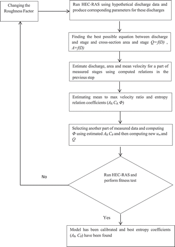
Combined methodology

This study proposed a simple but effective method for the estimation of mean velocity and discharge at ungauged sites by estimating the two coefficients of Equation (2)(2) ${\mathrm{\Phi }}_M=A_B\mathrm{I}\mathrm{n}\frac{B}{D}+C_B$(2) . Measurement of hydraulic parameters, such as water surface width, water depth and cross-sectional flow area in cross-sections, is easy, but the estimation of discharge needs mean velocity, u_m. The knowledge of M along with the measurement of u_max would allow the application of Equation (1)(1) ${\mathrm{\Phi }}_M=\frac{u_m}{u_{\mathrm{m}\mathrm{a}\mathrm{x}}}=\frac{e^M}{e^M-1}-\frac{1}{M}$(1) so that u_m can be estimated. In this case, an accurate estimate of M is necessary. For a gauged river site, M can be inferred if a robust dataset of pairs (u_m, u_max) is available. However, for ungauged sites M should be assessed in a different way. In this case, one could apply the method proposed by Moramarco and Singh (2010); however, it is necessary to know the hydrodynamic roughness length, y_o. To determine the value of Φ_M, we propose a method based on the coupling of Equation (2)(2) ${\mathrm{\Phi }}_M=A_B\mathrm{I}\mathrm{n}\frac{B}{D}+C_B$(2) and the hydraulic model HEC-RAS in an iterative loop. Hence, Equation (2)(2) ${\mathrm{\Phi }}_M=A_B\mathrm{I}\mathrm{n}\frac{B}{D}+C_B$(2) can be rewritten as:

(6) ${\mathrm{\Phi }}_{Mi}=A_B\mathrm{l}\mathrm{n}\frac{B_i}{D_i}+C_B$(6)

where B_i is the channel width corresponding to different flow depth, D_i. The object of this equation is to estimate A_B, C_B at an ungauged site, once the pairs (Φ_Mi, B_i/D_i) are plotted. The method consists of the following steps:

• Step 1. Assume that at the ungauged site only u_maxi is measured, at different water levels (D_i) and widths (B_i).

• Step 2. A Manning’s roughness is selected for HEC-RAS.

• Step 3. Using the selected Manning’s roughness, HEC-RAS is initialized by hypothetical steady discharge data, Q_i, and the corresponding B_i, A_i and D_i are estimated.

• Step 4. Based on Q_i, A_i and D_i, the relationships Q = f(D) and A = f(D) are identified using genetic programming.

• Step 5. The observed dataset of (u_maxi, D_i) at the site is split in two parts: Set 1 and Set 2.

• Step 6. From Set 1, the flow depth (D_i) and width (B_i) associated with each measure of u_maxi are considered. Discharge and area, according to the relationships obtained in Step 4, are assessed. Therefore, the mean velocity, u_mi and Φ_Mi for each of the stage values can be assessed as:

(7) $D_i,\to Q_i,A_i\to u_{mi}=\frac{Q}{A}\to {\varphi }_{Mi}=\frac{u_{mi}}{u_{\mathrm{m}\mathrm{a}\mathrm{x}i}}$(7)

• Step 7. A_B, C_B are estimated using Equation (2)(2) ${\mathrm{\Phi }}_M=A_B\mathrm{I}\mathrm{n}\frac{B}{D}+C_B$(2) , plotting the values for the pairs (B_i/D_i, Φ_Mi) computed in the previous step along with the observed D_i and B_i:

(8) ${\varphi }_M=A_B\mathrm{l}\mathrm{n}\frac{B_i}{D_i}+C_B\to A_B,C_B$(8)

• Step 8. From Set 2, B_j, D_j, A_j and u_maxj are considered. Then, Φ_Mj is estimated by applying in Equation (2)(2) ${\mathrm{\Phi }}_M=A_B\mathrm{I}\mathrm{n}\frac{B}{D}+C_B$(2) the values of A_B, C_B computed in the previous step and performing the processing as in the sequence:

(9) $B_j,D_j,\to {\varphi }_{Mj}=A_B\mathrm{l}\mathrm{n}\frac{B_j}{D_j}+C_B\to u_{mj}=u_{\mathrm{m}\mathrm{a}\mathrm{x}j}{\varphi }_{Mj}\to Q_j=u_{m_j}{A}_j$(9)

• Step 9. The Q_j values estimated in Step 8 are used as input to HEC-RAS and the new computed flow depths ($D_j^{\prime }$) at the river site are compared with the observed ones (D_j). Performance measures are assessed in terms of root mean square error (E_RMS) and mean absolute error (E_MA).

• Step 10. If optimal performance is not achieved, return to Step 1, modify Manning’s roughness and repeat steps 2–9.

Equation (2)(2) ${\mathrm{\Phi }}_M=A_B\mathrm{I}\mathrm{n}\frac{B}{D}+C_B$(2) proposes Φ_M = f(B/D); however, it would be interesting to estimate Φ_M, such as expressed also by Equation (1)(1) ${\mathrm{\Phi }}_M=\frac{u_m}{u_{\mathrm{m}\mathrm{a}\mathrm{x}}}=\frac{e^M}{e^M-1}-\frac{1}{M}$(1) . In this case, the procedure involves the same steps from 1 to 5, while steps 6–10 are as follows:

• Step 6. Select the measured D_i and u_maxi values from Set 1. The Q_i and A_i are estimated in accordance with the relationship identified in Step 4, from which the mean velocity is assessed as:

  (10) $D_i,\to Q_i,A_i\to u_{mi}=\frac{Q_i}{A_i}$(10)

• Step 7. As depicted in Equation (1)(1) ${\mathrm{\Phi }}_M=\frac{u_m}{u_{\mathrm{m}\mathrm{a}\mathrm{x}}}=\frac{e^M}{e^M-1}-\frac{1}{M}$(1) , find Φ_M by plotting the pairs (u_mi, u_maxi) of which u_maxi is the observed maximum velocity of Set 1.

• Step 8. Select from Set 2 the measured data u_maxj and D_j. Now proceed in reverse:

  (11) ${u_m}_j=u_{\mathrm{m}\mathrm{a}\mathrm{x}j}.{\mathrm{\Phi }}_M\to Q_j={u_m}_j.A_j$(11)

• Step 9. Using discharges estimated in (Step 8) above as inputs to HEC_RAS, the computed flow depths (D_j’) at the river site are compared with the observed depths (D_j) by assessing the performance measures.

• Step 10. If optimal performance is not achieved, return to Step 1, modify Manning’s roughness coefficient and repeat the above procedure.

The above steps involved in the procedure are depicted in Fig. 1. The proposed method was tested in both conditions using Ponte Nuovo data, and the results were compared.

Figure 1. Flowchart of the method

Performance measures

The performance of the proposed method was evaluated using three criteria: the coefficient of determination (R²), E_RMS and E_MA, expressed as follows:

(12) $R^2=1-\frac{{\sum }_{i=1}^n{\left({\left(X_{\mathrm{e}}\right)}_i-{\left({\mathrm{X}}_{\mathrm{o}}\right)}_i\right)}^2}{{\sum }_{i=1}^n{\left({\left(X_{\mathrm{e}}\right)}_i-X_{\mathrm{m}}\right)}^2}$(12)

(13) $E_{\mathrm{R}\mathrm{M}\mathrm{S}}=\sqrt{\frac{1}{n}{\sum }_{i=1}^n{\left({\left(X_{\mathrm{e}}\right)}_i-{\left(X_{\mathrm{o}}\right)}_i\right)}^2}$(13)

(14) $E_{\mathrm{M}\mathrm{A}}=\frac{1}{n}{\sum }_{i=0}^n\left.\left|{\left(X_o\right)}_i-{\left(X_e\right)}_i\right.\right|$(14)

where X₀ is the observed value, X_e is the value estimated by the proposed method and X_m is the mean of observed values.

In testing the method, X represents the flow depth, and after finding the best roughness factor, Φ_M, A_B and C_B, the method was tested using the mean velocity as X.

Results and discussion

Part of the Tiber River, including 18 cross-sections, was used for modelling; these cross-sections were obtained through a detailed topographical survey addressed to estimate the hydraulic and geometric characteristics of the gauged site based on velocity measurements. Moreover, a comparison of different topographical surveys at the gauged river site over several years also indicates that the river branch maintained a stable geometry throughout the measurements. Velocity measurements, carried out from a cableway by current meter during the last 20 years at Ponte Nuovo gauging site along the Tiber River, were analysed. The section subtends a basin of 4100 km², and the local bottom slope is 0.0014. The velocity dataset consists of velocity point data whose number along each sampled vertical is sufficient (more than eight for some verticals) to accurately reconstruct the vertical velocity profile. For each measurement, u_m and u_max are available along with the flow depth (D). In this study, 32 measurements were used and divided into two datasets of 16 measurements each. Table 1 shows the main hydraulic characteristics of the two datasets. The selection of the two sets was done in a random way. Using the observed flow depth as an indicator of performance, a Manning’s roughness coefficient equal to 0.04 s m^−1/3 for both main channel and flood plain produced the best results, and using genetic programming, the stage–discharge and stage–area relationships were computed in accordance with steps 1–10, yielding the following:

(15) $A=31.1{\left(D-0.019\right)}^{1.2}$(15)

(16) $Q=27.8{\left(D-0.84\right)}^{1.846}$(16)

Table 1. Range of variation of the main hydraulic characteristics of two datasets

	Q (m^3 s^−1)	D (m)	B (m)	UMAX (m s^−1)	UM (m s^−1)
Set 1	9–475	1.3–5.4	41–56	0.31–2.77	0.19–1.84
Set 2	7–497	1.3–5.95	42–57	0.22–2.69	0.14–1.82

Based on steps 5–10 of the procedure, the final relationship for Φ estimated as a function of the ratio between water width and water depth is:

(17) $\mathrm{\Phi }=1.119-0.1777\mathrm{l}\mathrm{n}\left(\frac{B}{D}\right)$(17)

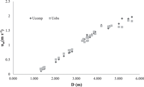
Since it was assumed that there were no measured data of mean velocity and discharge, for estimating Equation (17)(17) $\mathrm{\Phi }=1.119-0.1777\mathrm{l}\mathrm{n}\left(\frac{B}{D}\right)$(17) , the measured values of B, D and observed u_max were used. Therefore, the performance of the method was evaluated by comparing the computed and the observed mean velocity values. E_RMS and E_MA were found to be 0.09 m s⁻¹ and 0.06 m s⁻¹, respectively (Table 2). As shown in Fig. 2, the measured and estimated values of velocity were very close, indicating the good performance of the proposed method. 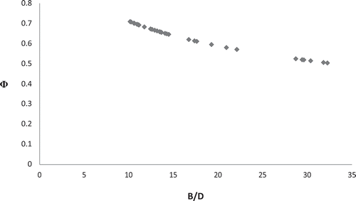Therefore, by having the values of water depth and channel width at the corresponding depth, it is possible to easily compute the values of Ф for any station using an equation (such as Equation (17)(17) $\mathrm{\Phi }=1.119-0.1777\mathrm{l}\mathrm{n}\left(\frac{B}{D}\right)$(17) ) and to compute the mean velocity and discharge using Ф values. Figure 3 shows the mean-to-maximum velocities ratio (Ф) vs. aspect ratio (B/D) for the Ponte Nuovo gauging site.

Table 2. Evaluation of the method, assuming Ф related to the ratio of water width to water depth

$R^2$	EMA (m s^−1)	ERMS (m s^−1)
0.98	0.06	0.09

Figure 2. Comparison between computed and observed mean velocity values by assuming Φ (Equation (17)(17) $\mathrm{\Phi }=1.119-0.1777\mathrm{l}\mathrm{n}\left(\frac{B}{D}\right)$(17) ) is related to the ratio of water width to water depth

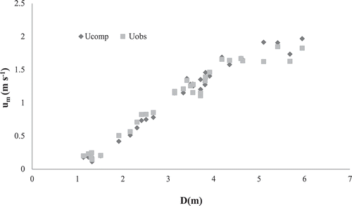
Figure 3. Ratio of mean to maximum velocities (Φ) vs. aspect ratio (B/D)

Following the procedure in which Ф was assumed to be constant (Steps 6–10), the slope of the best-fit line between u_mi and u_maxi was estimated to be equal to 0.67 (see Fig. 4). As shown in Fig. 5, the mean velocity values computed using Φ = 0.67 were very close to the observed values. The values of E_RMS and E_MA were found to be 0.08 and 0.05 m s⁻¹, respectively (Table 3). Therefore, according to the results, the method introduced in both cases has a good performance and can be used in situations where measured values of mean velocity are not available.

Table 3. Evaluation of the method in the second situation: Ф constant and computed equal to 0.67

$R^2$	EMA (m s^−1)	ERMS (m s^−1)
0.98	0.05	0.08

Figure 4. Mean velocity vs. maximum velocity computed by the proposed method

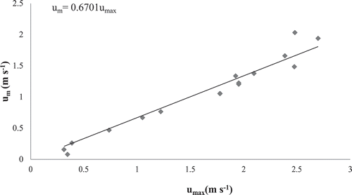
Figure 5. Comparison between computed and observed mean velocity values in the second situation (Φ = 0.67). D is observed water depth

Conclusion

In this study, a new and simple method based on a combination of hydraulic modelling (HEC-RAS), entropy-based velocity distribution, and one data-driven genetic programming technique to convert maximum velocity to mean velocity at ungauged stations is presented. The performance of this method was evaluated using two hypotheses of constant and non-constant entropy parameter Φ expressed as a function of the width-to-depth ratio. In the two cases, results were similar and accurate, based on the performance measures, at the Ponte Nuovo site. Therefore, the method can be conveniently adopted to estimate the entropy quantity Φ starting from easy measurements of hydraulic variables (water depth, channel width and maximum velocity), even during high floods. However, more river sites need to be considered to further test the method, and for that, new data on natural channels with different geometric and hydraulic characteristics will need to be collected.

Acknowledgements

This work has been partly supported by the Italian National Research Programme PRIN 2017, with the project “Interactions between hydrodynamics flows and biotic communities in fluvial ecosystems: advancement in discharge monitoring and understanding of processes relevant for ecosystem sustainability by the development of novel technologies with field observations and laboratory testing (ENTERPRISING).”

Disclosure statement

No potential conflict of interest was reported by the authors.

References

- Bathurst, J.C., 1985. Flow resistance estimation in mountain rivers. Journal of Hydraulic Engineering, 111 (4), 625–643. doi:10.1061/(ASCE)0733-9429(1985)111:4(625)
- Bathurst, J.C., Li, R.M., and Simons, D.B., 1981. Resistance equation for large-scale roughness. Journal of the Hydraulics Division, 107 (HY12), 1593–1613.
- Chiu, C.L., 1987. Entropy and probability concepts in hydraulics. Journal of Hydraulic Engineering, 113 (5), 583–600. doi:10.1061/(ASCE)0733-9429(1987)113:5(583)
- Farina, G., et al., 2014. Three methods for estimating the entropy parameter M based on a decreasing number of velocity measurements in a river cross-section. Entropy, 16 (5), 2512–2529. doi:10.3390/e16052512
- Ferro, V., 2003. ADV measurements of velocity distributions in a gravel bed flume. Earth Surface Processes and Landforms, 28 (7), 707–722. doi:10.1002/esp.467
- Greco, M., 2015. Effect of bed roughness on 1-D entropy velocity distribution in open channel flow. Hydrology Research, 46 (1), 1–10. doi:10.2166/nh.2013.122
- Greco, M., 2016. Entropy-based approach for rating curve assessment in rough and smooth irrigation ditches. Journal of Irrigation and Drainage Engineering, 142 (3), 04015062. doi:10.1061/(ASCE)IR.1943-4774.0000986
- Greco, M. and Mirauda, D., 2015. An entropy based velocity profile for steady flows with large-scale roughness. In: G. Lollino, et al., eds. Engineering geology for society and territory - volume 3. Cham: Springer, 641–645.
- Greco, M., Mirauda, D., and Volpe Plantamura, A., 2014. Manning’s roughness through the entropy parameter for steady open channel flows in low submergence. Procedia Engineering, 70, 773–780. doi:10.1016/j.proeng.2014.02.084
- Greco, M. and Moramarco, T., 2015. Influence of bed roughness and cross section geometry on medium and maximum velocity ratio in open-channel flow. Journal of Hydraulic Engineering, 06015015. doi:10.1061/(ASCE)HY.1943-7900.0001064
- Griffiths, G.A., 1980. Hydraulic geometry relationships of some New Zealand gravel-bed rivers. Journal of Hydrology (New Zealand), 19 (2), 106–118.
- Leopold, L.B. and Maddock, T., 1953. The hydraulic geometry of stream channels and some physiographic implications. Geological Survey Professional Paper 252. Washington,DC: U.S. Dept. of the Interior.
- Leopold, L.B., Wolman, M.G., and Miller, J.P., 1964. Fluvial processes in geomorphology. San Francisco: W. H. Freeman and Company, 522.
- Moramarco, T., Barbetta, S., and Tarpanelli, A., 2017. From surface flow velocity measurements to discharge assessment by the entropy theory. Water, 9 (2), 120. doi:10.3390/w9020120
- Moramarco, T., Saltalippi, C., and Singh, V.P., 2004. Estimation of mean velocity in natural channels based on Chiu’s velocity distribution equation. Journal of Hydrologic Engineering, 9 (1), 42–50. doi:10.1061/(ASCE)1084-0699(2004)9:1(42)
- Moramarco, T. and Singh, V.P., 2010. Formulation of the entropy parameter based on hydraulic and geometric characteristics of river cross sections. Journal of Hydrologic Engineering, 15 (10), 852–858. doi:10.1061/(ASCE)HE.1943-5584.0000255
- Xia, R., 1997. Relation between mean and maximum velocities in a natural river. Journal of Hydrologic Engineering., 13 (8), 720–723. doi:10.1061/(ASCE)0733-9429(1997)123:8(720)
- Yang, H.Y., et al., 2014. An indirect approach for discharge estimation: A combination among micro-genetic algorithm, hydraulic model, and in situ measurement. Flow Measurement and Instrumentation, 39, 46–53. doi:10.1016/j.flowmeasinst.2014.07.003
- Yang, S.Q., Tan, S.K., and Lim, S.Y., 2004. Velocity distribution and dip-phenomenon in smooth uniform open channel flows. Journal of Hydraulic Engineering, 130 (12), 1179–1186. doi:10.1061/(ASCE)0733-9429(2004)130:12(1179)