Evaluation of a stochastic weather generator for long-term ensemble streamflow forecasts

ABSTRACT

Resampling historical time series remains one of the main approaches used to generate long-term probabilistic streamflow forecasts, while there is a need to develop more flexible approaches taking into account non-stationarities. One possible approach is to use a modelling chain consisting of a stochastic weather generator and a hydrological model. However, the ability of this modelling chain to generate adequate probabilistic streamflows must first be evaluated. The aim of this paper is to compare the performance of a stochastic weather generator against resampling historical meteorological time series in order to produce ensemble streamflow forecasts. The comparison framework is based on 30 years of forecasts for a single Canadian watershed. Forecasts resulting from the two methods are evaluated using the continuous ranked probability score (CRPS) and rank histograms. Results indicate that while there are differences between the methods, they nevertheless perform similarly, thus showing that weather generators can be used as substitutes for resampling the historical past.

KEYWORDS:

• stochastic weather generator
• resampling
• ensemble streamflow forecast
• long term

Editor A. Fiori Associate editor A. Requena

1 Introduction

Long-term streamflow forecasting (1–12 months ahead) is important to various water resource sectors, such as hydropower generation and optimal reservoir operation (Georgakakos 1989, Hamlet et al. 2002, Markoff and Cullen 2008). Consequently, providing reliable long-term streamflow forecasts has long been a concern for the hydrological science community.

A main issue with long-term streamflow forecasts involves properly incorporating uncertainties that grow larger as the forecast lead time increases (Georgakakos 1989). Deterministic forecasts have long been used, but have proven to be inadequate for long-term forecasts, and this has led researchers to focus on probabilistic approaches to properly encompass the large uncertainties associated with distant forecasts. An ensemble prediction system (ESP; Cooke 1906, Weather Bureau Brier 1944, Murphy and Winkler 1984, Day 1985) is a collection of two or more forecasts over the same future horizon, which represents the various probability states and uncertainties associated with the forecasting process (Sivillo et al. 1997). Various studies have demonstrated the benefit of using ESP in reservoir management and in the decision-making process (Faber and Stedinger 2001, Kim et al. 2007, Zhao et al. 2013). ESP is now widely used in research and operational forecasts around the world (Cloke and Pappenberger 2009).

The methods for making probabilistic forecasts can be classified into three main categories, namely numerical weather prediction systems (NWPs), resampling methods and stochastic weather generators (WGs). NWPs, obtained by assimilating current atmospheric and oceanic conditions into a coupled numerical mathematical model, are the most accurate tool for forecasting future weather conditions (Pielke 2013). However, forecasts from NWPs typically have skill up to a 6-day horizon for low precipitation (less than 2 mm) and for up to 4 days for high precipitation (between 2 and 10 mm) (Chen et al. 2010). NWPs are therefore not well suited for hydrological forecasts with longer time horizons as they cannot adequately represent long-term forecast uncertainty (Coulibaly 2003, Cloke and Pappenberger 2009). Accordingly, long-term forecasts typically favour resampling of the historical past as well as the use of WGs. Seasonal weather forecasts from coupled numerical models, both calibrated and uncalibrated, are currently receiving a lot of attention with the potential of outperforming ESP depending on season, region and lead time (Yuan 2016, Bennett et al. 2017, Arnal et al. 2018). However, resampling remains by far the most commonly used operational approach when it comes to generating long-term forecasts and estimating forecast uncertainties (Todorovic and Woolhiser 1975, Young 1994, Leander and Buishand 2009, King et al. 2014).

Resampling approaches were developed around 1990 to alleviate the problems inherent in parametric models (Lall and Sharma 1996), with one main such problem being the assumption of normality, which is not realized for most hydrological variables. This assumption requires data transformation, which is a primary cause of bias (Lall and Sharma 1996, Sharma et al. 1997, Prairie et al. 2006). In addition, parametric methods often have difficulties representing the complex nonlinear relationships observed between hydrometeorological variables. This weakness is what led to the development of nonparametric resampling methods, such as the index sequential method (ISM), the kernel-based approach and k-Nearest Neighbors (K-NN) bootstrapping methods (Kendall and Dracup 1991, Sharma and Sharma 1997, Salas and Lee 2009, Sharifazari and Araghinejad 2015, Li et al. 2017, Khaki et al. 2018). Although widely used thanks to their relative ease of implementation, most resampling approaches do, however, suffer from the same potential drawbacks.

Resampling methods are based on the historical record, and any deficiency in this record will affect the forecast quality. The methods are also unable to generate weather values larger (or smaller) than observed values (Rajagopalan and Lall 1999), which limits their ability to properly assess uncertainty related to rare events. The length of the historical record also brings limitations when it comes to appropriately sampling forecast uncertainty. Finally, non-stationarities due to internal climate variability and anthropogenic change call into question the validity of using the historical past for accurate long-term streamflow forecasts (Murphy and Winkler 1984, Clark et al. 2004a, 2004b). Despite all the different methods and techniques that have been proposed over the years, additional research is still needed to fully address these issues (Lall 1995, Prairie et al. 2006, 2007, Lee et al. 2010).

Stochastic WGs were developed in the 1980s with the aim of generating long-enough synthetic weather time series with specific statistical properties to be used in hydrologic models and risk assessment studies, and to extend and simulate weather time series at locations with no observed data (Wilks and Wilby 1999). The long time series of WGs have been used in many applications such as flood type classification (Turkington et al. 2016) and simulation of extreme floods (Okoli et al. 2019, Výleta and Valent 2019, Winter et al. 2019, Sikorska-Senoner et al. 2020) up to the probable maximum flood (Chen et al. 2015), as well as in many climate change studies (Semenov and Barrow 1997, Keller et al. 2017, Steinschneider et al. 2019, Ahn 2020). Many other studies have focused on improving WGs to represent higher statistical moments of both univariate and multivariate statistics of observed weather data (Hayhoe 2000, Hansen and Mavromatis 2001, Kyselý and Dubrovský 2005, Brissette et al. 2007, Chen et al. 2012a). Other studies have also looked into using WGs as constituting a downscaling tool in climate change impact studies because of the relative ease with which their parameters can be modified to represent climate variability (Semenov and Barrow 1997, Kilsby et al. 2007, Zhuang et al. 2016, Keller et al. 2017). Despite this advantage, only a few studies have looked at the potential of using stochastic WGs for long-term streamflow forecasting (Li et al. 2013, Breinl et al. 2015, Shield and Dai 2015, Breinl 2016), and an even smaller number implemented a WG into streamflow forecasts. Of note, Šípek and Daňhelka (2015) used a WG for ESP based on a limited number of observed years selected on the basis of large-scale climate indices, and Hwang et al. (2011) generated several precipitation scenarios to study the impact of uncertainty on streamflow simulations. Both studies pointed to the potential of WGs for improving ESP.

WGs have the potential to overcome the main drawbacks of resampling approaches and, notably, to take into account non-stationarities. Resampling approaches are much less flexible due to the limited number of years available. Before moving on to the evaluation of approaches dealing with non-stationarity, a necessary first step is to evaluate the ability of a stochastic WG for generating ensemble streamflow forecasts. Therefore, the goal of this paper is to compare the performance of ensemble streamflow forecasts built from resampling the historical record against that of a stochastic WG when coupled with a hydrological model to provide long-term probabilistic streamflow forecasts.

The remainder of this paper is divided into four sections. The watershed and data are first described, followed by the methodology employed. Results are then presented and discussed in the last two sections.

2 Description of watershed and data

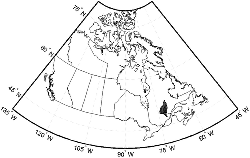
The Lac Saint-Jean watershed was selected as a test case for this study. It is located in the eastern Canadian province of Quebec (Fig. 1). It has a surface area of 73 800 km² and consists of four main rivers flowing into a 1000 km² lake (Lac Saint-Jean), which is regulated at its outlet by a large hydropower dam. Rio Tinto, the world’s largest producer of aluminium, operates six power plants on this watershed, with an annual average capacity of 2000 megawatts, feeding a large aluminium plant. Economic development around Lac Saint-Jean is therefore closely linked to its hydropower potential (Dibike and Coulibaly 2005). Overall, the watershed is sparsely inhabited, and its land cover mostly consists of a homogeneous boreal forest.

Figure 1. Lac Saint-Jean watershed. W: West; N: North

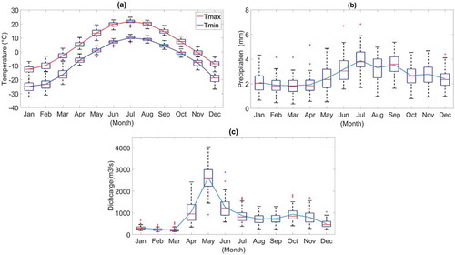
Daily precipitation, daily maximum and minimum temperatures are provided in gridded format by the Natural Resources Canada (NRCAN) dataset. NRCAN is the only high-resolution Canada-wide daily-scale precipitation and temperature gridded dataset. It provides daily values with a 10-km spatial resolution (300 arcseconds). The NRCAN dataset is interpolated from the Canadian network of gauge surface stations using trivariate thin-plate smoothing splines, providing continuous functions as a function of latitude, longitude and ground-surface elevation (Hutchinson et al. 2009). The study period covered in this work spans the years 1950 to 2010. Daily scale naturalized streamflow data for Lac Saint-Jean was provided by Rio-Tinto, and covers the same time period. Figure 2 presents the annual cycle (and variability) of the hydrometeorological variables used in this study. Temperature and streamflow values are characterized by a strong seasonal pattern typical of a northern latitude climate, whereas the precipitation values show a weaker cycle with increased mean monthly totals in the summer and early fall.

Figure 2. Annual cycle of key hydrometeorological variables used in this study. (a) Minimum and maximum temperatures; (b) precipitation; (c) streamflow

3 Methodology

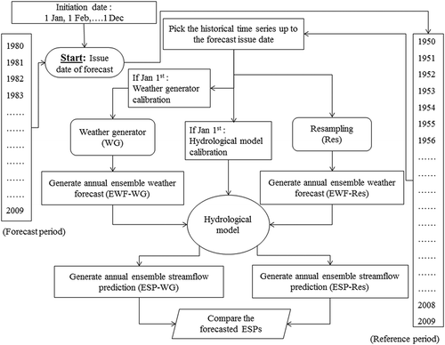
The aim of this project is to compare the performance of WGs against the benchmark method of equiprobable resampling for long-term streamflow forecasting. To this end, the framework for this comparison consists of three main steps. In the first step, for each forecast date, ensemble weather forecasts are generated from both approaches. In the second step, these weather forecasts are used with a hydrological model to generate ensemble streamflow forecasts. In the last step, the forecasts from both methods are compared against observed past conditions. Details are provided below.

Both methods are evaluated in hindcast mode over the 30-year, 1980–2009 period. The 1950–1979 time period is used as the initial historical record. Over the evaluation period, 1-year-ahead forecasts are made 12 times per year, on the first day of each month. The evaluation period therefore comprises 360 1-year forecasts (30 years × 12 forecasts). Similarly to what would be done in the real world, the recalibration of the hydrological model and WG is performed at the beginning of every new year, adding the preceding year to the historical record. Figure 3 presents the methodological framework.

Figure 3. Methodological framework

3.1 Ensemble weather forecast: approach 1 – resampling

In this study, the simple method of resampling the past observed climatology data is used as the benchmark approach. As discussed earlier, resampling past climatology is the most commonly used approach for long-term ensemble weather forecasting. This work uses equiprobable resampling with no reshuffling between precipitation and temperature years. The number of members in each of the ensemble weather forecasts is therefore equal to the number of years in the historical period.

3.2 Ensemble weather forecast: approach 2 – stochastic WG

The WG used in this study is WeaGETS, the uni-site multivariate WG (Chen et al. 2012a). WeaGETS is based on the original work of Richardson (1981) and Richardson and Wright (1984). It first generates precipitation occurrence using a first-, second- or third-order Markov chain. On wet days, precipitation is then generated using either an exponential or a gamma distribution. Minimum and maximum temperatures are generated conditionally on the wet/dry day status. Serial correlation and cross-correlations between precipitation and temperature are preserved using a first-order autoregressive process. Inter- and intra-annual variability is preserved using the spectral approach of Chen et al. (2010). All WeaGETS parameters are first computed on a monthly basis, and are then interpolated to the daily scale with Fourier harmonics, as proposed by Richardson (Richardson 1981) More details can be found in Chen et al. (2010, 2012a). For this study, a first-order Markov chain is used to produce the precipitation occurrence, and the two-parameter gamma distribution is used for estimating precipitation amounts. The gamma distribution has been used in many studies to model precipitation in a WG (Chen et al. 2016). It performs generally well but often fails at generating extreme precipitation that follows a distribution with a heavier tail, such as the generalized extreme value distribution (GEV) or Generalized Pareto distributions. Accordingly, several studies have compared various distribution functions to be used in WGs (Li et al. 2013, Breinl 2016, Breinl et al. 2017, Li and Shi 2019). These studies typically find that the more complex distribution functions, with three or more parameters, outperform the simpler ones, especially for larger quantiles of the observed distributions. However, for a study of long-term hydrological forecasts, the gamma distribution was deemed adequate. In addition, for large catchments such as the one under study, the impact of extreme convective precipitation on part of the catchment is lessened by the averaging of the streamflow-generating processes at the watershed scale.

Like most WGs, WeaGETS can generate an extremely large number of years (limited by computer storage/memory); 500 members were generated for each forecast. We used multiple randomly selected samples of N years to explore the impact of the number of members, but no significant difference was observed. Therefore, to allow for a fair comparison, for all forecasts the number of WG members is always identical to the number of years available in the historical past. Prior to using the WG, precipitation, minimum and maximum temperatures were averaged using all NRCAN grid points within the catchment boundaries. Despite the size of the catchment, a unisite WG (as opposed to a more complex multisite WG) was chosen because of the catchment’s very uniform topography and land cover (boreal forest). Despite the high spatial resolution of the NRCAN gridded dataset, the underlying station network over this high-latitude watershed is very sparse, and did not justify the use of a more complex multisite WG. In addition, Chen et al. (2016) showed that using a multisite WG on this same catchment did not result in any improvement in hydrological modelling, when compared to its simpler counterpart. In general, overparameterized methods may not always perform well, and the simpler methods are often preferred by operational agencies.

3.3 Hydrological model

The hydrological model used in this study is the lumped conceptual Service Hydrométéorologique Apports Modules Intermédiaires (HSAMI) model. HSAMI was developed by Hydro-Québec, and is used to make hourly and daily operational forecasts for more than 80 watersheds with surface areas ranging between 160 and 70,000 km². It has also been used in many Canadian hydrological studies, including climate change impact studies (Minville et al. 2008, Chen et al. 2011), multi-model simulations (Arsenault et al. 2015), model calibration experiments (Arsenault et al. 2013) and regionalization studies (Arsenault and Brissette 2014a, 2014b). HSAMI is a conceptual rainfall–runoff lumped model with 23 parameters. Two parameters account for evapotranspiration, 6 parameters for snowmelt simulation and 15 parameters for vertical and horizontal water movement. Vertical water flows are estimated by four interconnected linear reservoirs (snow on the ground; surface water; saturated and unsaturated zones). Horizontal routing is carried out by two unit hydrographs and one linear reservoir for low flows. The minimum required inputs are daily scale precipitation, maximum and minimum temperature, and flow discharge for the calibration period. If available, cloud cover fraction and snow water equivalent can also be used as inputs. The calibration of HSAMI was performed automatically using the covariance matrix adaptation evolution strategy (CMA-ES) algorithm (following the work of Arsenault et al. (2013)), with the Nash-Sutcliffe criterion used as an objective function. The calibration process followed the procedure outlined in Arsenault et al. (2018), and bypassed the validation step.

To avoid any bias resulting from the hydrological model, and to forgo the complex assimilation process, simulated streamflows were used instead of observations. Doing so results in a “perfect” hydrological model and eliminates all uncertainties resulting from the assimilation process and hydrological modelling biases. This ensures that all differences between the resampling and WG ensemble streamflow forecasts are entirely due to differences in the generation of the ensemble weather forecasts.

3.4 Evaluation procedure

The challenge for all probabilistic forecasts is to provide an unbiased ensemble with the proper dispersion. Despite the steadily growing body of literature on ensemble streamflow forecasting, the number of evaluation metrics remains relatively small. The main probabilistic score broadly used in the meteorological and hydrological community for ensemble verification remains the continuous ranked probability score (CRPS; Matheson and Winkler 1976). The CRPS generalizes the mean absolute error (MAE) to the case of probabilistic forecasts.

If F is the predictive cumulative distribution function (CDF) and y is the observation, the CRPS can be defined by:

(1) $\mathrm{C}\mathrm{R}\mathrm{P}\mathrm{S}\left(F,y\right)=\underset{-\mathrm{\infty }}{\overset{\mathrm{\infty }}{\int }}{\left[F\left(t\right)-H\left(t-y\right)\right]}^2\mathrm{d}\mathrm{t}$(1)

where $H\left(t-y\right)$ is the Heaviside function. It is 0 when $t<y$, and 1 otherwise (Hersbach 2000, Toth et al. 2003).

A perfect CRPS value is zero (all members of the ensemble predicting the same value, equal to the observation) and, therefore, the aim of a probabilistic forecast is to minimize the CRPS value. The CRPS allows for discrimination between different ensemble forecasts.

Another important part of ensemble verification is related to the dispersion of the forecast. To this end, the rank histogram (Talagrand diagram) has been widely used as a graphical evaluation method to visually assess the bias and spread of an ensemble forecast. The rank histogram measures how well the ensemble forecast represents the probabilistic distribution of observations (Hamill 2001). To plot the rank histogram, the forecast is typically separated into n + 1 bins (with n being the number of members in an ensemble), and a count is tabulated for the number of times observations fall within each bin. For a perfect ensemble forecast, the rank histogram will be flat since the probability of the observation falling within each bin would be equal. Alternatively, the number of bins can be related to the CDF of the ensemble. An asymmetrical rank histogram is the result of a biased forecast, whereas concave or concave shapes represent, respectively, an under- or over-dispersed forecast (Hersbach 2000, Hamill 2001, Wilks 2006, Zalachori et al. 2012). To measure the deviation from the flat and uniform rank histogram, the flatness coefficient (δ) described in Equation (2)(2) $\delta =\frac{1}{n+1}\sum _{z=1}^{z=n+1}\left|f\left(z\right)-y\right|$(2) is used:

(2) $\delta =\frac{1}{n+1}\sum _{z=1}^{z=n+1}\left|f\left(z\right)-y\right|$(2)

where $f\left(z\right)$ is the relative frequency in rank $z,y=\frac{1}{n+1}$ is the theoretical relative frequency, and $n$ is the number of ensemble members.

In a perfectly flat rank histogram, the value of δ is equal to 0 (Velázquez et al. 2010).

4 Results

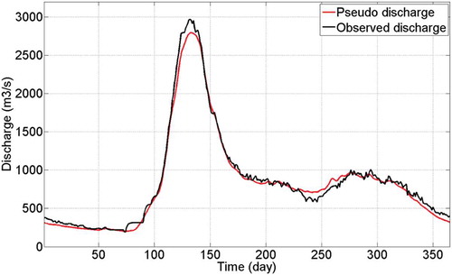
Prior to using the modelled streamflows as pseudo-observations, it is nonetheless important to ensure that HSAMI performs accurately over the Lac Saint-Jean watershed. Figure 4 shows the mean hydrograph derived from observation and modelled streamflows over the 1950–1980 period. The performance of HSAMI is excellent (Nash-Sutcliffe of mean daily hydrograph is 0.9885) and justifies the use of a conceptual lumped model, despite the large size of the Lac Saint-Jean watershed. This performance also justifies the use of a single-site WG, rather than its more complex multi-site version (Brissette et al. 2007, Chen et al. 2014).

Figure 4. Mean annual hydrograph of simulated and observed inflows into Lac Saint-Jean

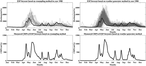
As was shown in the methodology framework, the ESP forecasts are made by two methods at each forecast date and over the entire forecast period. CRPS values are calculated daily for each forecast. Figure 5 shows the ensemble streamflow forecasts made on 1 January 1980, and the associated CRPS values for both forecast approaches. The larger apparent spread observed for the WG is because all 500 generated members were used to plot this figure. For the comparison of all forecasts, the first N members (between 30 and 59 depending on the hindcast year) of the generated ensemble were chosen, as discussed earlier. Otherwise, the two approaches provide forecasts with similar CRPS values.

Figure 5. One-year ensemble streamflow forecasts made on 1 January 1980 using resampling (left) and weather generator (right) approaches. The black line represents observations. There are 30 members for resampling (1950–1979) and 500 members for the weather generator (first row). The CRPS values are shown in the second row

Figure 6 presents mean monthly CRPS values aggregated across all forecasts. Twelve 1-year forecasts are made for every year, one on the first of each month. The mean monthly CRPS value is computed for each year by taking the mean of each daily CRPS (30 days × 12 forecasts). The box plots presented in Fig. 6 are made with the mean monthly CRPS values computed for each forecasted year (1980–2009). Values are then used to construct the box plots. The solid box plot rectangles represent the interquartile spread (25th and 75th quantiles), with the median near the middle, while the whiskers show the extent of the values. Outliers are identified with the + sign.

Figure 6. Box plot results of monthly CRPS based on ESPs forecasted by resampling and the weather generator method on 1 January, 1 April, 1 July and 1 October

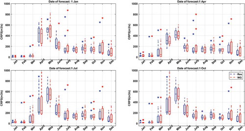
These results indicate that the two forecasting approaches perform similarly in all cases. The largest CRPS values are observed during the spring flood in April, May and June, when uncertainty and streamflow values are at their maximum, whereas the lowest values are related to the winter low flows, where uncertainty and streamflow values are relatively small. The impact of the forecast date on CRPS values is quite clear when looking at the 1 April forecast, which results in lower uncertainty in the spring flood. To better outline differences between the two forecasting approaches, Fig. 7 presents the 30-year average of all mean monthly CRPS values for all 12 forecast dates.

Figure 7. Mean monthly CRPS of ensemble streamflow forecasts using the resampling (top) and weather generator (bottom) approaches

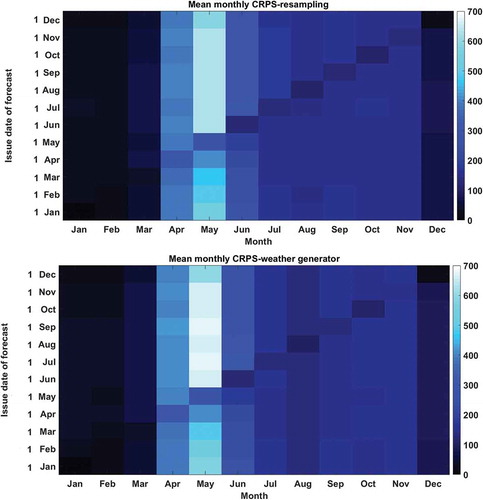
As was the case for Fig. 6, the mean monthly values are obtained by averaging daily CRPS values within each month, for all 30 years of the hindcasting period and all 12 forecast dates. Therefore, each mean monthly value represents the average for 360 forecasted days. The vertical axis presents the date of the forecast, and the horizontal axis shows the month of the forecast. Accordingly, the diagonal is distinctly darker since it corresponds to the first month of each forecasting date, when uncertainty is lowest. The general pattern of the mean monthly CRPS is very similar for both approaches. The lowest mean monthly CRPS values are consistently found in the winter, when the streamflows are consistently small. Mean monthly CRPS values are highest during the snowmelt period (April to June), when streamflow values and variability are highest. To better outline differences between the two approaches, Fig. 8 presents the difference between the estimates of mean monthly CRPS values.

Figure 8. Difference between the mean monthly continuous ranked probability score (CRPS) values from the resampling and weather generator approaches. Red indicates that the resampling approach has a lower mean monthly CRPS, while blue indicates the reverse

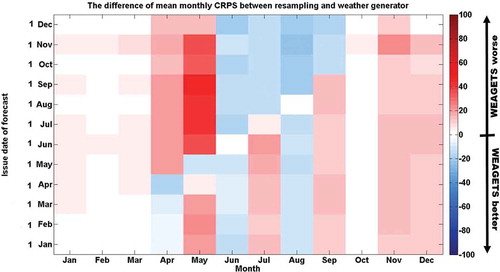
The difference between the two approaches is minimal from January to March. The resampling forecast ensemble performs generally better in April and May, especially for longer lead times (above the diagonal). The WG approach generally gives lower mean monthly CRPS values in the summer, but consistently larger ones in November and December. Nonetheless, differences remain small, with the exception of May forecasts issued 7–12 months in advance.

To further compare the two approaches, rank histograms are presented in Figs. 9 and 10. Each histogram is composed of 10 800 forecasted days (30 days per month × 12 1-year forecasts × 30 years). The histogram flatness value (Equation 3) is presented within each histogram figure.

Figure 9. Plotted rank histograms based on monthly ESP forecasts using the resampling method

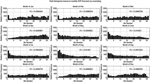
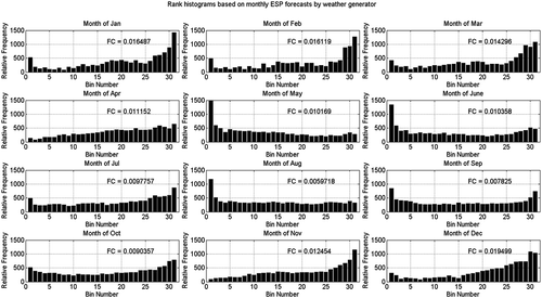
Figure 10. Plotted rank histograms based on monthly ESP forecasts using the weather generator method

A constant number of 30 ensemble members were used for all forecasts. The WG randomly generated 30 years for each forecasting date. For resampling, when the number of historical years was larger than 30, the ensemble members were chosen randomly from amongst all available years.

Overall, all histograms are relatively flat. All forecasts for both approaches are relatively well dispersed. There is, however, one main difference between the two approaches. Despite having similar mean CRPS values (Figs. 6 and 7), the rank histograms for the WG approach display a small but consistent negative bias for the winter months (November to March), with flatness values consistently higher than for the resampling values. The two approaches otherwise perform similarly during all other months, although resampling results in a larger positive bias during the post-flood period, from May to November.

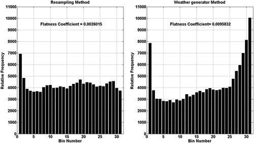
Finally, Fig. 11 presents the rank histogram of all 1-year monthly forecasts made from 1 January 1980 to 31 December 2009. The resampling rank histogram is flat, with a very slight positive bias. Taken globally, the results indicate that the WG’s performance is not nearly as good as resampling, as it is negatively biased and slightly under-dispersed.

Figure 11. Global rank histogram pooled from all 1-year monthly forecasts for the resampling (left) and weather generator (right) approaches

5 Discussion

The results presented are based on 360 1-year forecasts issued on the first of each month, from January 1980 to December 2009. Overall, the results, presented in terms of CRPS and rank histograms, show that the two approaches perform similarly. In terms of the CRPS metric, the two approaches are globally equivalent. The WG method generates slightly better forecasts just before the flood (January to April), whereas resampling is generally slightly better for the forecasts issued after the flood. The performance is also similar when looking at bias and dispersion from rank histograms, although the WG forecasts are globally slightly under-dispersed and negatively biased. This shows the importance of using more than one metric to evaluate forecast quality (Hamill 2001, Renner et al. 2009, Demargne et al. 2010). The differences between the two approaches remain small, and become clearer after all forecasts are pooled together (Fig. 11). The reasons for the differences are difficult to explain. In principle, stochastic WGs are built to reproduce uni- and multivariate statistics of observed time series. The WG used in this work has been extensively tested for its ability to reproduce characteristics of precipitation and temperature series (Caron et al. 2008, Li et al. 2010, Chen et al. 2014), and especially for its ability to correct for the underestimation of intra- and inter-annual variance (Chen et al. 2010). To better understand the reasons behind this behaviour, we plotted rank histograms of accumulated precipitation at 3, 6, 9 and 12 months, as shown in Fig. 12.

Figure 12. Rank histograms of accumulated precipitation at 3, 6, 9 and 12 months from the weather generator (left) and resampling (right) approaches

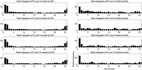
This shows that the WG precipitation is under-dispersed and slightly negatively biased, which tracks well with the results observed for streamflow as displayed in Fig. 11. This appears to result from an underestimation of the temporal autocorrelation of precipitation by the WG. The structure of WeaGETS does not specifically prescribe the temporal autocorrelation of precipitation, and all other requirements (e.g. preserve wet/day series, cross-correlations with temperature) are not sufficient to induce a temporal autocorrelation. The variance correction scheme of Chen et al. (2010) preserves inter-annual autocorrelation but does not address it at the intra-annual scale, which is most important for streamflow forecasts. Figure 13 presents CRPS of monthly precipitation for both the WG and resampling.

Figure 13. Mean monthly CRPS box plots for the 1-year, 1 January forecast over the entire 30-year hindcast period, 1980–2009

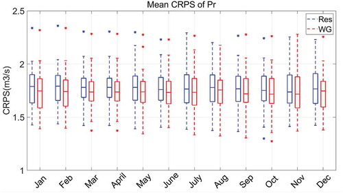
The results show that the WG CRPS values are slightly better than those from resampling, which is consistent with the results of Fig. 6 for streamflows. A similar exercise was performed for temperature (results not shown) and no noticeable difference was found between resampling and WG outputs. In the case of temperature, the WG uses an autoregressive scheme which specifically mandates temporal autocorrelation of the generated time series. It therefore appears that most of the observed differences can be tracked to the underestimation of intra-annual precipitation autocorrelation by the WG.

The performance of WG outputs in terms of driving environmental models (such as a hydrology model) has been less studied in the literature, even though this is one of the main reasons why WGs were developed in the first place. Such studies performed with hydrological models indicate that WG series provide realistic streamflow series for a wide variety of conditions. The small differences observed between WGs and original observed series however can be increased due to the impact of hydrological model (Khalili et al. 2011, Li et al. 2013). The results presented in this work are consistent with these findings, in that WG streamflow forecasts appear to perform similarly to those from resampling, but with some relatively minor differences that are difficult to track back to the WG precipitation and temperature time series. The hydrological model acts as a complex non-linear filter of precipitation and temperature, and small changes in one or both series may result in somewhat larger differences. If the WG time series were statistically identical to the observed series, one would expect the two streamflow ensembles to perform identically. Any differences can therefore be tracked back to minor inadequacies in the WG series characteristics.

The presence of biases in forecasts is typically rooted in uncertainties due to a combination of various input, output, model structure and parameter uncertainties (Krzysztofowicz 2002, Han et al. 2007, Li et al. 2009). Such biases have been noted in resampled time series in other studies (Seo et al. 2006, Schaake et al. 2007, Bogner and Kalas 2008). In particular, biases in long-term forecasts may be due to the non-stationarities present in historical time series (Ceola et al. 2014, Meng et al. 2019) due to internal climate variability and long-term trends linked to anthropogenic forcing.

Non-stationarity in hydro climatic time series is now well documented in many regions of the world (Westra et al. 2013). Non-stationarity raises important questions about equiprobable historical resampling. Using non-equiprobable resampling is a complex endeavour, for which there is currently no easy solution. It is, however, relatively easy to incorporate non-stationarity into a stochastic WG. A few studies have provided frameworks that could be applied to the problem of generating long-term ensemble streamflow forecasts (Semenov and Barrow 1997, Chen et al. 2012b, Jones et al. 2016, Keller et al. 2017, Li Liu et al. 2017). For example, the variability structure of historical meteorological time series at seasonal, monthly and daily scales could be preserved, while mean annual and seasonal values could be conditioned on large-scale teleconnection indices or by weighting years differently, with the more recent ones being more important. Comparatively, resampling approaches are much less flexible due to the limited number of years available. If the historical record is long enough, non-equiprobable resampling offers the possibility of selecting a subset of years judged more relevant based on criteria such as similarity to current/recent conditions (e.g. wet, warm) or based on a limited number of climate indices (e.g. El Niño Southern Oscillation). Such selection is, however, far from simple, and the “less relevant” years left out of the process may still contain important information on internal climate variability that would be useful to long-term forecasts. A WG could be used to generate stochastic variability around a small subset of years based on the similarity to present climate indices, as was done by Šípek and Daňhelka (2015), for example. In practice, however, correlations between climate indices are typically small in many regions of the world.

In any event, approaches dealing with climate non-stationarity for long-term streamflow forecasting must recognize the two main components of climate change: internal variability and anthropogenic forcing. Internal or unforced variability comes from the chaotic behaviour of the climate system, and impacts the regional climate at seasonal to multidecadal scales. Internal variability is most often represented by patterns of precipitation and temperature anomalies at local and regional scales. Anthropogenic forcing results from the increase in greenhouse gas emissions) and results in slow but steady changes in the climate. For temperature, anthropogenic forcing already displays a clear signature, with warming exceeding 2°C annually at high latitudes, and has exceeded that due to internal variability in most parts of the world (Lehner et al. 2017), whereas for precipitation, internal variability is expected to remain the dominant variability component until later this century (Martel et al. 2018). Incorporating temperature and precipitation non-stationarity into long-term streamflow forecasts should therefore follow a different process for each variable.

6 Conclusion

This paper presents a comparison of two methods for generating long-term ensemble streamflow forecasts. Both methods make use of a hydrological model to transform precipitation and temperature time series into streamflows. The first approach resamples historical time series, while the second makes use of a stochastic WG calibrated using the same historical series. The main goal of this paper is therefore to validate the use of a stochastic WG for ensemble streamflow forecasting. To this end, forecasts made from the combination of a stochastic WG and a hydrological model are compared to those obtained from equiprobable resampling of past meteorological variables. The evaluation period consisted of 1-year-long forecasts issued on the first day of each month over a 30-year hindcast period (1980–2009). Forecasts resulting from the two methods are evaluated with respect to CRPS and rank histograms.

Results indicate that while there are differences between the two methods, they largely perform similarly, which thus indicates that WGs can be used as substitutes for resampling the historical past. Potential approaches to modify WGs to take into account non-stationarities are discussed.

Acknowledgements

This research project was supported by the Natural Sciences and Engineering Research Council of Canada (NSERC) through a Collaborative Research and Development (CRD) Grant, and by Hydro-Québec, Rio Tinto and the Ouranos Consortium on Regional Climatology and Adaptation to Climate Change. The authors acknowledge Korbinian Breinl (Vienna University of Technology) and an anonymous reviewer for their constructive comments on this article.

Disclosure statement

No potential conflict of interest was reported by the authors.

Additional information

Funding

This work was supported by the Natural Sciences and Engineering Research Council of Canada (NSERC) [CRNSG # RDCPJ 428468 – 11].

References

- Ahn, K.-H., 2020. Coupled annual and daily multivariate and multisite stochastic weather generator to preserve low-and high-frequency variability to assess climate vulnerability. Journal of Hydrology, 581, 124443. doi:10.1016/j.jhydrol.2019.124443
- Arnal, L., et al., 2018. Skilful seasonal forecasts of streamflow over Europe? Hydrology and Earth System Sciences, 22, 2057–2072. doi:10.5194/hess-22-2057-2018
- Arsenault, R., et al., 2013. Comparison of stochastic optimization algorithms in hydrological model calibration. Journal of Hydrologic Engineering, 19, 1374–1384. doi:10.1061/(ASCE)HE.1943-5584.0000938
- Arsenault, R., et al., 2015. A comparative analysis of 9 multi-model averaging approaches in hydrological continuous streamflow simulation. Journal of Hydrology, 529, 754–767. doi:10.1016/j.jhydrol.2015.09.001
- Arsenault, R. and Brissette, F., 2014a. Determining the optimal spatial distribution of weather station networks for hydrological modeling purposes using RCM datasets: an experimental approach. Journal of Hydrometeorology, 15, 517–526. doi:10.1175/JHM-D-13-088.1
- Arsenault, R., Brissette, F., and Martel, J.-L., 2018. The hazards of split-sample validation in hydrological model calibration. Journal of Hydrology, 566, 346–362. doi:10.1016/j.jhydrol.2018.09.027
- Arsenault, R. and Brissette, F.P., 2014b. Continuous streamflow prediction in ungauged basins: the effects of equifinality and parameter set selection on uncertainty in regionalization approaches. Water Resources Research, 50, 6135–6153. doi:10.1002/2013WR014898
- Bennett, J.C., et al., 2017. Assessment of an ensemble seasonal streamflow forecasting system for Australia. Hydrology and Earth System Sciences, 21, 6007–6030. doi:10.5194/hess-21-6007-2017
- Bogner, K. and Kalas, M., 2008. Error‐correction methods and evaluation of an ensemble based hydrological forecasting system for the Upper Danube catchment. Atmospheric Science Letters, 9, 95–102. doi:10.1002/asl.180
- Breinl, K., 2016. Driving a lumped hydrological model with precipitation output from weather generators of different complexity. Hydrological Sciences Journal, 61, 1395–1414. doi:10.1080/02626667.2015.1036755
- Breinl, K., et al., 2017. Can weather generation capture precipitation patterns across different climates, spatial scales and under data scarcity? Scientific Reports, 7, 1–12. doi:10.1038/s41598-017-05822-y
- Breinl, K., Turkington, T., and Stowasser, M., 2015. Simulating daily precipitation and temperature: a weather generation framework for assessing hydrometeorological hazards. Meteorological Applications, 22, 334–347. doi:10.1002/met.1459
- Brissette, F., Khalili, M., and Leconte, R., 2007. Efficient stochastic generation of multi-site synthetic precipitation data. Journal of Hydrology, 345, 121–133. doi:10.1016/j.jhydrol.2007.06.035
- Caron, A., Leconte, R., and Brissette, F., 2008. An improved stochastic weather generator for hydrological impact studies. Canadian Water Resources Journal, 33, 233–256. doi:10.4296/cwrj3303233
- Ceola, S., Montanari, A., and Koutsoyiannis, D., 2014. Toward a theoretical framework for integrated modeling of hydrological change. Wiley Interdisciplinary Reviews: Water, 1, 427–438. doi:10.1002/wat2.1038
- Chen, J., et al., 2011. Overall uncertainty study of the hydrological impacts of climate change for a Canadian watershed. Water Resources Research, 47, 47. doi:10.1029/2010WR009451
- Chen, J., Brissette, F., and Leconte, R., 2012a. WeaGETS–a Matlab-based daily scale weather generator for generating precipitation and temperature. Procedia Environmental Sciences, 13, 2222–2235. doi:10.1016/j.proenv.2012.01.211
- Chen, J., Brissette, F.P., and Leconte, R., 2010. A daily stochastic weather generator for preserving low-frequency of climate variability. Journal of Hydrology, 388, 480–490. doi:10.1016/j.jhydrol.2010.05.032
- Chen, J., Brissette, F.P., and Leconte, R., 2012b. Downscaling of weather generator parameters to quantify hydrological impacts of climate change. Climate Research, 51, 185–200. doi:10.3354/cr01062
- Chen, J., Brissette, F.P., and Zhang, X.J., 2014. A multi-site stochastic weather generator for daily precipitation and temperature. Transactions of the ASABE, 57, 1375–1391.
- Chen, J., Brissette, F.P., and Zhang, X.J., 2016. Hydrological modeling using a multisite stochastic weather generator. Journal of Hydrologic Engineering, 21, 04015060. doi:10.1061/(ASCE)HE.1943-5584.0001288
- Chen, J., Brissette, F.P., and Zielinski, P.A., 2015. Constraining frequency distributions with the probable maximum precipitation for the stochastic generation of realistic extreme events. Journal of Extreme Events, 2, 1550009. doi:10.1142/S2345737615500098
- Clark, M., et al., 2004a. The Schaake shuffle: a method for reconstructing space–time variability in forecasted precipitation and temperature fields. Journal of Hydrometeorology, 5, 243–262. doi:10.1175/1525-7541(2004)005<0243:TSSAMF>2.0.CO;2
- Clark, M.P., et al., 2004b. A resampling procedure for generating conditioned daily weather sequences. Water Resources Research, 40(4).
- Cloke, H. and Pappenberger, F., 2009. Ensemble flood forecasting: a review. Journal of Hydrology, 375, 613–626. doi:10.1016/j.jhydrol.2009.06.005
- Cooke, E., 1906. Forecasts and verifications in Western Australia. Monthly Weather Review, 34, 23–24. doi:10.1175/1520-0493(1906)34<23:FAVIWA>2.0.CO;2
- Coulibaly, P., 2003. Impact of meteorological predictions on real‐time spring flow forecasting. Hydrological Processes, 17, 3791–3801. doi:10.1002/hyp.5168
- Day, G.N., 1985. Extended streamflow forecasting using NWSRFS. Journal of Water Resources Planning and Management, 111, 157–170. doi:10.1061/(ASCE)0733-9496(1985)111:2(157)
- Demargne, J., et al., 2010. Diagnostic verification of hydrometeorological and hydrologic ensembles. Atmospheric Science Letters, 11, 114–122. doi:10.1002/asl.261
- Dibike, Y.B. and Coulibaly, P., 2005. Hydrologic impact of climate change in the Saguenay watershed: comparison of downscaling methods and hydrologic models. Journal of Hydrology, 307, 145–163. doi:10.1016/j.jhydrol.2004.10.012
- Faber, B.A. and Stedinger, J., 2001. Reservoir optimization using sampling SDP with ensemble streamflow prediction (ESP) forecasts. Journal of Hydrology, 249, 113–133. doi:10.1016/S0022-1694(01)00419-X
- Georgakakos, A.P., 1989. The value of streamflow forecasting in reservoir operation 1. JAWRA Journal of the American Water Resources Association, 25, 789–800. doi:10.1111/j.1752-1688.1989.tb05394.x
- Hamill, T.M., 2001. Interpretation of rank histograms for verifying ensemble forecasts. Monthly Weather Review, 129, 550–560. doi:10.1175/1520-0493(2001)129<0550:IORHFV>2.0.CO;2
- Hamlet, A.F., Huppert, D., and Lettenmaier, D.P., 2002. Economic value of long-lead streamflow forecasts for Columbia river hydropower. Journal of Water Resources Planning and Management, 128, 91–101. doi:10.1061/(ASCE)0733-9496(2002)128:2(91)
- Han, D., Kwong, T., and Li, S., 2007. Uncertainties in real‐time flood forecasting with neural networks. Hydrological Processes: An International Journal, 21, 223–228. doi:10.1002/hyp.6184
- Hansen, J.W. and Mavromatis, T., 2001. Correcting low-frequency variability bias in stochastic weather generators. Agricultural and Forest Meteorology, 109, 297–310. doi:10.1016/S0168-1923(01)00271-4
- Hayhoe, H.N., 2000. Improvements of stochastic weather data generators for diverse climates. Climate Research, 14, 75–87. doi:10.3354/cr014075
- Hersbach, H., 2000. Decomposition of the continuous ranked probability score for ensemble prediction systems. Weather and Forecasting, 15, 559–570. doi:10.1175/1520-0434(2000)015<0559:DOTCRP>2.0.CO;2
- Hutchinson, M.F., et al., 2009. Development and testing of Canada-wide interpolated spatial models of daily minimum–maximum temperature and precipitation for 1961–2003. Journal of Applied Meteorology and Climatology, 48, 725–741. doi:10.1175/2008JAMC1979.1
- Hwang, Y., Clark, M.P., and Rajagopalan, B., 2011. Use of daily precipitation uncertainties in streamflow simulation and forecast. Stochastic Environmental Research and Risk Assessment, 25, 957–972. doi:10.1007/s00477-011-0460-1
- Jones, P., et al., 2016. Downscaling regional climate model outputs for the Caribbean using a weather generator. International Journal of Climatology, 36, 4141–4163. doi:10.1002/joc.4624
- Keller, D. E., et al., 2017. Testing a weather generator for downscaling climate change projections over Switzerland. International Journal of Climatology, 37, 928–942.
- Kendall, D.R. and Dracup, J.A., 1991. A comparison of index-sequential and AR (1) generated hydrologic sequences. Journal of Hydrology, 122, 335–352. doi:10.1016/0022-1694(91)90187-M
- Khaki, M., et al., 2018. Nonparametric data assimilation scheme for land hydrological applications. Water Resources Research, 54, 4946–4964. doi:10.1029/2018WR022854
- Khalili, M., Brissette, F., and Leconte, R., 2011. Effectiveness of multi‐site weather generator for hydrological modeling 1. JAWRA Journal of the American Water Resources Association, 47, 303–314. doi:10.1111/j.1752-1688.2010.00514.x
- Kilsby, C., et al., 2007. A daily weather generator for use in climate change studies. Environmental Modelling and Software, 22, 1705–1719. doi:10.1016/j.envsoft.2007.02.005
- Kim, Y.-O., et al., 2007. Optimizing operational policies of a Korean multireservoir system using sampling stochastic dynamic programming with ensemble streamflow prediction. Journal of Water Resources Planning and Management, 133, 4–14. doi:10.1061/(ASCE)0733-9496(2007)133:1(4)
- King, L.M., Mcleod, A.I., and Simonovic, S.P., 2014. Simulation of historical temperatures using a multi‐site, multivariate block resampling algorithm with perturbation. Hydrological Processes, 28, 905–912. doi:10.1002/hyp.9596
- Krzysztofowicz, R., 2002. Bayesian system for probabilistic river stage forecasting. Journal of Hydrology, 268, 16–40. doi:10.1016/S0022-1694(02)00106-3
- Kyselý, J. and Dubrovský, M., 2005. Simulation of extreme temperature events by a stochastic weather generator: effects of interdiurnal and interannual variability reproduction. International Journal of Climatology, 25, 251–269. doi:10.1002/joc.1120
- Lall, U., 1995. Recent advances in nonparametric function estimation: hydrologic applications. Reviews of Geophysics, 33, 1093–1102. doi:10.1029/95RG00343
- Lall, U. and Sharma, A., 1996. A nearest neighbor bootstrap for resampling hydrologic time series. Water Resources Research, 32, 679–693. doi:10.1029/95WR02966
- Leander, R. and Buishand, T.A., 2009. A daily weather generator based on a two-stage resampling algorithm. Journal of Hydrology, 374, 185–195. doi:10.1016/j.jhydrol.2009.06.010
- Lee, T., Salas, J., and Prairie, J., 2010. An enhanced nonparametric streamflow disaggregation model with genetic algorithm. Water Resources Research, 46, 46. doi:10.1029/2009WR008375
- Lehner, F., et al., 2017. Projected drought risk in 1.5 C and 2 C warmer climates. Geophysical Research Letters, 44, 7419–7428. doi:10.1002/2017GL074117
- Li, H., et al., 2009. The role of initial conditions and forcing uncertainties in seasonal hydrologic forecasting. Journal of Geophysical Research: Atmospheres, 114 (D4), D04114.
- Li, L., et al., 2010. Streamflow forecast and reservoir operation performance assessment under climate change. Water Resources Management, 24, 83. doi:10.1007/s11269-009-9438-x
- Li Liu, D., et al., 2017. Effects of different climate downscaling methods on the assessment of climate change impacts on wheat cropping systems. Climatic Change, 144, 687–701. doi:10.1007/s10584-017-2054-5
- Li, W., et al., 2017. A review on statistical postprocessing methods for hydrometeorological ensemble forecasting. Wiley Interdisciplinary Reviews: Water, 4, e1246. doi:10.1002/wat2.1246
- Li, Z., Brissette, F., and Chen, J., 2013. Finding the most appropriate precipitation probability distribution for stochastic weather generation and hydrological modelling in Nordic watersheds. Hydrological Processes, 27 (25), 3718–3729. doi:10.1002/hyp.9499
- Li, Z. and Shi, X., 2019. Stochastic generation of daily precipitation considering diverse model complexity and climates. Theoretical and Applied Climatology, 137, 839–853. doi:10.1007/s00704-018-2638-7
- Markoff, M.S. and Cullen, A.C., 2008. Impact of climate change on Pacific Northwest hydropower. Climatic Change, 87, 451–469. doi:10.1007/s10584-007-9306-8
- Martel, J.-L., et al., 2018. Role of natural climate variability in the detection of anthropogenic climate change signal for mean and extreme precipitation at local and regional scales. Journal of Climate, 31, 4241–4263. doi:10.1175/JCLI-D-17-0282.1
- Matheson, J.E. and Winkler, R.L., 1976. Scoring rules for continuous probability distributions. Management Science, 22, 1087–1096. doi:10.1287/mnsc.22.10.1087
- Meng, E., et al., 2019. A robust method for non-stationary streamflow prediction based on improved EMD-SVM model. Journal of Hydrology, 568, 462–478. doi:10.1016/j.jhydrol.2018.11.015
- Minville, M., Brissette, F., and Leconte, R., 2008. Uncertainty of the impact of climate change on the hydrology of a nordic watershed. Journal of Hydrology, 358, 70–83. doi:10.1016/j.jhydrol.2008.05.033
- Murphy, A.H. and Winkler, R.L., 1984. Probability forecasting in meteorology. Journal of the American Statistical Association, 79, 489–500.
- Okoli, K., et al., 2019. A systematic comparison of statistical and hydrological methods for design flood estimation. Hydrology Research, 50, 1665–1678. doi:10.2166/nh.2019.188
- Pielke, Sr, R.A., 2013. Mesoscale meteorological modeling. New York: Academic press.
- Prairie, J., et al., 2007. A stochastic nonparametric technique for space‐time disaggregation of streamflows. Water Resources Research, 43, 43. doi:10.1029/2005wr004773
- Prairie, J.R., et al., 2006. Modified K-NN model for stochastic streamflow simulation. Journal of Hydrologic Engineering, 11, 371–378. doi:10.1061/(ASCE)1084-0699(2006)11:4(371)
- Rajagopalan, B. and Lall, U., 1999. A k‐nearest‐neighbor simulator for daily precipitation and other weather variables. Water Resources Research, 35, 3089–3101. doi:10.1029/1999WR900028
- Renner, M., et al., 2009. Verification of ensemble flow forecasts for the River Rhine. Journal of Hydrology, 376, 463–475. doi:10.1016/j.jhydrol.2009.07.059
- Richardson, C.W., 1981. Stochastic simulation of daily precipitation, temperature, and solar radiation. Water Resources Research, 17, 182–190. doi:10.1029/WR017i001p00182
- Richardson, C.W. and Wright, D.A., 1984. WGEN: a model for generating daily weather variables. Washington, DC: U.S. Department of Agriculture, Agricultural Research Service, ARS-8.
- Salas, J.D. and Lee, T., 2009. Nonparametric simulation of single-site seasonal streamflows. Journal of Hydrologic Engineering, 15, 284–296. doi:10.1061/(ASCE)HE.1943-5584.0000189
- Schaake, J.C., et al., 2007. HEPEX: the hydrological ensemble prediction experiment. Bulletin of the American Meteorological Society, 88, 1541–1548. doi:10.1175/BAMS-88-10-1541
- Semenov, M.A. and Barrow, E.M., 1997. Use of a stochastic weather generator in the development of climate change scenarios. Climatic Change, 35, 397–414. doi:10.1023/A:1005342632279
- Seo, D.-J., Herr, H., and Schaake, J., 2006. A statistical post-processor for accounting of hydrologic uncertainty in short-range ensemble streamflow prediction. Hydrology and Earth System Sciences Discussions, 3, 1987–2035. doi:10.5194/hessd-3-1987-2006
- Sharifazari, S. and Araghinejad, S., 2015. Development of a nonparametric model for multivariate hydrological monthly series simulation considering climate change impacts. Water Resources Management, 29, 5309–5322. doi:10.1007/s11269-015-1119-3
- Sharma, A. and Sharma, U.S., 1997. Liposomes in drug delivery: progress and limitations. International Journal of Pharmaceutics, 154, 123–140. doi:10.1016/S0378-5173(97)00135-X
- Sharma, A., Tarboton, D.G., and Lall, U., 1997. Streamflow simulation: a nonparametric approach. Water Resources Research, 33, 291–308. doi:10.1029/96WR02839
- Shield, S. and Dai, Z. 2015. Comparison of uncertainty of two precipitation prediction models. arXiv preprint arXiv:1508.03662.
- Sikorska-Senoner, A.E., Schaefli, B., and Seibert, J., 2020. Downsizing parameter ensembles for simulations of extreme floods. Natural Hazards and Earth System Sciences, 20 (12), 3521–3549.
- Šípek, V. and Daňhelka, J., 2015. Modification of input datasets for the Ensemble Streamflow Prediction based on large-scale climatic indices and weather generator. Journal of Hydrology, 528, 720–733. doi:10.1016/j.jhydrol.2015.07.008
- Sivillo, J.K., Ahlquist, J.E., and Toth, Z., 1997. An ensemble forecasting primer. Weather and Forecasting, 12, 809–818. doi:10.1175/1520-0434(1997)012<0809:AEFP>2.0.CO;2
- Steinschneider, S., et al., 2019. A weather‐regime‐based stochastic weather generator for climate vulnerability assessments of water systems in the Western United States. Water Resources Research, 55, 6923–6945. doi:10.1029/2018WR024446
- Todorovic, P. and Woolhiser, D.A., 1975. A stochastic model of n-day precipitation. Journal of Applied Meteorology, 14, 17–24. doi:10.1175/1520-0450(1975)014<0017:ASMODP>2.0.CO;2
- Toth, Z., et al., 2003. Probability and ensemble forecasts. In: I.T. Jolliffe and D.B. Stephenson, eds. Forecast verification: a practitioner's guide in atmospheric science. Wiley, 137–163.
- Turkington, T., et al., 2016. A new flood type classification method for use in climate change impact studies. Weather and Climate Extremes, 14, 1–16. doi:10.1016/j.wace.2016.10.001
- Velázquez, J., Anctil, F., and Perrin, C., 2010. Performance and reliability of multimodel hydrological ensemble simulations based on seventeen lumped models and a thousand catchments. Hydrology and Earth System Sciences, 14, 2303–2317. doi:10.5194/hess-14-2303-2010
- Výleta, R. and Valent, P., 2019. A methodology for continuous a flood frequency analysis with weather generator and rainfall-runoff model. Geophysical Research Abstracts, vol. 21.
- Weather Bureau Brier, G.W., 1944. Verification of a Forecaster’s confidence and the use of probability statements in weather forecasting. US Department of Commerce, Weather Bureau, Res. Pap. No. 16.
- Westra, S., Alexander, L.V., and Zwiers, F.W., 2013. Global increasing trends in annual maximum daily precipitation. Journal of Climate, 26, 3904–3918. doi:10.1175/JCLI-D-12-00502.1
- Wilks, D., 2006. On “field significance” and the false discovery rate. Journal of Applied Meteorology and Climatology, 45, 1181–1189. doi:10.1175/JAM2404.1
- Wilks, D.S. and Wilby, R.L., 1999. The weather generation game: a review of stochastic weather models. Progress in Physical Geography, 23, 329–357. doi:10.1177/030913339902300302
- Winter, B., et al., 2019. A continuous modelling approach for design flood estimation on sub-daily time scale. Hydrological Sciences Journal, 64, 539–554. doi:10.1080/02626667.2019.1593419
- Young, K.C., 1994. A multivariate chain model for simulating climatic parameters from daily data. Journal of Applied Meteorology, 33 (6), 661–671. doi:10.1175/1520-0450(1994)033<0661:AMCMFS>2.0.CO;2
- Yuan, X., 2016. An experimental seasonal hydrological forecasting system over the Yellow River basin–Part 2: the added value from climate forecast models. Hydrology and Earth System Sciences (Online), 20 (6), 2453–2466.
- Zalachori, I., et al., 2012. Statistical processing of forecasts for hydrological ensemble prediction: a comparative study of different bias correction strategies. Advances in Science and Research, 8, 135–141. doi:10.5194/asr-8-135-2012
- Zhao, T., et al., 2013. Generalized martingale model of the uncertainty evolution of streamflow forecasts. Advances in Water Resources, 57, 41–51. doi:10.1016/j.advwatres.2013.03.008
- Zhuang, X., et al., 2016. Assessment of climate change impacts on watershed in cold-arid region: an integrated multi-GCM-based stochastic weather generator and stepwise cluster analysis method. Climate Dynamics, 47, 191–209.