On coupled dynamics and regime shifts in coupled human–water systems

ABSTRACT

Social and hydrological dynamics are coupled, nonlinear, and complex. To clarify and enhance our understanding of such dynamics, we developed a stylized model that combines hydrological and social dynamics of a generic coupled human–water system. In this model, neither too much water (flood) nor too little water (drought) is desirable, and the population self-organizes to respond to relative benefits they derive from the water system and outside opportunities. Despite its simplicity, the model yields seven different regimes, governed by hydrological and socioeconomic factors. As external drivers change, the conditions giving rise to these regimes shift, and with them social consequences such as migration patterns. A clear understanding of the regime boundaries (thresholds) derived from this simple model contributes to insights on how one might cope with a complex socio-hydrological system under change.

KEYWORDS:

• coupled human–water systems
• social-ecological systems
• dynamical system modeling
• regime shift
• thresholds
• socio-hydrology

Editor S. Archfield; Associate editor D. Yu

1 Introduction

Human societies interact with hydrologic systems to meet their needs – from water supply, flood control, and hydropower to agricultural production and environmental demand (Gunderson et al. 2017). This interaction alters the hydrological dynamics in these coupled human–water systems (CHWSs) (Querner 2000, Bonacci et al. 2016, Mittal et al. 2016). Understanding the interplay between the societal and hydrologic systems is essential to avoid transitioning into undesirable regimes (Montanari et al. 2013, Thompson et al. 2013). The sustainability of CHWSs is linked to these regime shifts (Van De Meene et al. 2011, Wang et al. 2017), whose nature is shaped by climatic, hydrologic, and societal drivers (e.g. floods, droughts, wars, economic collapses; Black et al. 2011, Sivapalan et al. 2012). Regime shifts caused by such drivers have a long history dating back several thousand years; for example, an extended drought period may have caused the collapse of the Maya civilization (Hodell et al. 1995, Haug et al. 2003). Regime shifts in CHWSs can also lead to many drastic consequences, among the most dramatic of which is migration (Warziniack 2013): water wars are becoming a reality, leading to the mass movement of environmental refugees (Basok 1993, Selby and Hoffmann 2012, Jägerskog and Swain 2016). These regime shifts pose challenges to the governance of CHWSs, rendering sustainability more difficult to attain even when the driver that triggered the shift has been reduced or removed (Scheffer et al. 2001, Carpenter and Kinne 2003). Therefore, identifying the boundaries and understanding the characteristics of different regimes in a CHWS are crucial for its sustainable management.

In recent decades, the subject of ecological thresholds and regime shifts has drawn much attention among scientists (Muradian 2001, Scheffer et al. 2001, Folke et al. 2004, Biggs et al. 2009, 2018, Lade et al. 2013, Bauch et al. 2016, Nayak and Armitage 2018). However, there is still room to improve our understanding of the dynamic behavior of CHWSs and the effects of social and environmental drivers on the sustainability of these complex systems (Sivapalan et al. 2012). While studies on regime shifts have been on the rise in the past two decades, regime shifts specific to CHWSs have been under-studied. For example, evaluating six North American water basins, Gunderson et al. (2017) found that in these highly managed water resource systems, river development has increased wealth but undermined ecosystem functions, which could lead to deterioration of resilience against climate change. In another study, Coutinho et al. (2015) investigated possible regime shifts of the main reservoir serving the metropolitan area of São Paulo, Brazil. These studies highlighted the importance of identifying possible regimes in CHWSs. It is our objective to obtain a clearer understanding of such thresholds and regimes in CHWSs.

A wide range of approaches to identify ecological thresholds and regime shifts have been developed over the years (Zeileis et al. 2003, Mantua 2004, Rodionov 2005, Carpenter and Brock 2006, Andersen et al. 2009). Some statistical approaches depend on time series of observed data to infer the ecological regime shift (Schröder et al. 2005) and “are so data demanding that only exceptionally few long-term ecological data sets would meet the requirements” (Andersen et al. 2009, p. 55). Such data requirements are particularly challenging for studying regime shifts in CHWSs, which need to go beyond the effects of climatic and hydrological drivers (Deyoung et al. 2008) and include social drivers such as economic opportunities, overpopulation, and overexploitation. Mantua (2004) reviewed a number of other analytical methods for detecting regime shifts in large marine systems and discussed their relative strengths and weaknesses. These approaches often suffer from the inability to capture nonlinear relationships (Jolliffe and Cadima 2016) and the possibility of detecting a regime shift when none exists (Rudnick and Davis 2003).

In this paper, we adopt a dynamical system modeling approach, which relies on internal dynamics, feedbacks, constraints, and boundary conditions to represent the nonlinear behavior of a system (Hengl et al. 2007). Dynamical system modeling allows for systematic scrutiny of the effects of different drivers, individually or in combination, on regime shifts and evaluates the resilience and robustness of the system. Additionally, possible early warning signals for the regime shift may be inferred from such a model (e.g. Lade et al. 2013). Specifically, we developed a stylized dynamical system model to study regime shifts of a generic CHWS. The model enables us to identify and delineate the boundaries between different regimes. We then analyzed the model to investigate the effects of social and natural drivers (e.g. labor market conditions and climate change) to obtain a clearer understanding of thresholds and regimes in CHWSs.

This paper is organized as follows. Section 2 briefly describes the model. Section 3 reports and discusses the model results, with more details on the derivations and properties of equilibrium points associated with different regimes reported in the Appendix. Finally, section 4 summarizes the significant contributions and key findings of this study.

2 Model description

The stylized model developed is a two-dimensional (2D) system, with the two variables being the amount of water storage (S) in a CHWS, either naturally or in reservoirs, and the fraction of effort a user spends inside the system (V). S depends on the inflow to the system, natural loss, and water consumption rate. On the social side, every user has two choices, either staying inside the system for payoff π or leaving the system to earn w outside the system. Table 1 summarizes the model’s variables and parameters.

Table 1. Definitions and dimensions of variables and parameters

Symbol	Definition	Unit
S	Water storage in the system	[S]
V	Fraction of effort a user spends inside the system	[-]
t	Time	[T]
π	Payoff to a user per unit time	[$/NT]
w	Per user revenue for working outside	[$/NT]
N	Number of water users	[N]
r’	Responsiveness of water users to payoff difference	[N/$]
r	Water withdrawal rate per user	[1/NT]
l	Natural loss rate	[1/T]
a’, b’	Utility equation coefficients	[S/NT]
X	Production rate per user	[Z/NT]
p	Price of unit produced	[$/Z]
U	Utility of water use	[-]

S: water storage; T: time; N: population size; Z: unit of product.

Essentially, the dynamics of S is based on the mass balance of inflow and natural loss, with human extraction added; this type of formulation is commonly used in traditional bioeconomic models. Specifically, the dynamics of S is assumed to be:

(1) $\frac{dS}{dt}=I-rNVS-lS$(1)

where I is the natural inflow rate to the system, N is the total number of users, r represents the withdrawal rate per user, and l is the natural loss rate. The water extraction by the users is thus rNVS, and the natural loss is lS.

To capture the dynamics of the strategic behaviors of water users, we used the replicator equation. According to Cressman and Tao (2014, p. 10810), the “replicator equation is the first and most important game dynamics studied in connection with evolutionary game theory to capture social learning.” Replicator dynamics captures simple social learning mechanisms in which each user/agent observes and replicates strategies with better payoffs, without requiring an unrealistic assumption of unbounded rationality on the users’ part (see, e.g. Schuster and Sigmund 1983, Hofbauer and Sigmund 2003, Nowak 2006, Cressman and Tao 2014). In replicator dynamics, it is assumed that users base their decision on limited information – in this case, other users’ strategies and their payoffs – as opposed to a full rational analysis of the entire payoff structure. Many scholars have used such formulations to analyze social behavior in modeling social-ecological systems (Lade et al. 2013, Lafuite et al. 2017, Tilman et al. 2017, Bury et al. 2019). Here we assumed the dynamics of V to be

(2) $\frac{dV}{dt}=r{ }^{\mathrm{\prime }}V\left(1-V\right)\left(\pi -w\right)$(2)

where $r{ }^{\mathrm{\prime }}$ is the responsiveness of users to the payoff difference; with the same payoff difference, higher $r{ }^{\mathrm{\prime }}$ results in a greater magnitude of dV/dt. The replicator equation shows how V changes in response to the incentive-based driver. When the per capita payoff of working inside the system, π, is higher than the per capita payoff of alternative opportunities, w, V increases, and vice versa. On the flip side, (1 − V)N can be thought of as a proxy for the number of people emigrating from the system to find outside opportunities.

Here, we define the per capita payoff, π, as

(3) $\pi =XpU$(3)

where X is the unit of production (e.g. of an agricultural community) per user, and p is the unit price of such product. The utility function, U, represents the level of satisfaction of users, which depends on the amount of water a user receives. U varies between 0, the lowest level of satisfaction, and 1, the highest level. Therefore, Xp can be thought of as the maximum payoff users obtain when they receive an optimal level of water (no drought, no flood). Here, we represent U with the following truncated inverted quadratic function (Fig. 1):

(4) $U=U\left(S\right)=\left\{\begin{array}{c}4\left(\frac{Sr-a{ }^{\mathrm{\prime }}}{b{ }^{\mathrm{\prime }}-a^{\prime }}\right)\left(\frac{b{ }^{\mathrm{\prime }}-Sr}{b{ }^{\mathrm{\prime }}-a^{\prime }}\right),a{ }^{\mathrm{\prime }}<Sr<b^{\prime }\\ 0,\mathrm{o}\mathrm{t}\mathrm{h}\mathrm{e}\mathrm{r}\mathrm{w}\mathrm{i}\mathrm{s}\mathrm{e}\end{array}\right.$(4)

Figure 1. Utility function. Utility function of a water user with respect to the received water: $a{ }^{\mathrm{\prime }}$indicates the lower threshold below which the utility function is zero. $b{ }^{\mathrm{\prime }}$ is the higher threshold above which the utility function is zero

where Sr is the water share each water user receives (dividing the water assigned to all users, rNVS, by the number of water users, VN); and $a{ }^{\mathrm{\prime }}$ and $b{ }^{\mathrm{\prime }}$ are the parameters of the utility function: $a{ }^{\mathrm{\prime }}$ represents the lower threshold below which the level of satisfaction is zero (think drought), and $b{ }^{\mathrm{\prime }}$ represents the upper threshold above which the users are no longer satisfied (think flood). This characteristic – too much or too little is not desirable – is more salient for water than for other natural resources. This nonmonotonicity is one of the features that make this study different from some previous work (e.g. Yu et al. 2014, Muneepeerakul and Anderies 2017, 2020) in which utility/payoff was a non-decreasing function of a resource.

It should be noted that although the model’s formulation may be more suited to local communities where the members are engaged in management and maintenance of the water resource, the model still offers some applicable insights for other socio-hydrological systems to the extent that the human extraction term and the utility function can capture what is going on in those systems. Many people living in cities depend directly or indirectly on water-dependent industries; in those cases, instead of migration, low $V^{\ast }$ may be interpreted as people switching from a water-dependent sector/industry to a less water-sensitive one. Of course, these other systems would have other characteristics that modulate the interplay between water and utility and are not captured in this model.

To simplify the analysis, we non-dimensionalized Equations (1)(1) $\frac{dS}{dt}=I-rNVS-lS$(1) and (2(2) $\frac{dV}{dt}=r{ }^{\mathrm{\prime }}V\left(1-V\right)\left(\pi -w\right)$(2) ) as follows:

(5) $\begin{array}{c}\frac{ds}{d\tau }=1-Vs-\alpha s\\ \\ \frac{dV}{d\tau }=\beta V\left(1-V\right)\left(U-\mu \right)\end{array}$(5)

See Table 2 for the definitions and interpretation of the dimensionless groups used in the above equations. The utility function U is now rewritten in terms of the dimensionless groups as follows:

(6) $U=U\left(s\right)=\left\{\begin{array}{c}4\left(\frac{s-a}{b-a}\right)\left(\frac{b-s}{b-a}\right),a<s<b\\ 0,\mathrm{o}\mathrm{t}\mathrm{h}\mathrm{e}\mathrm{r}\mathrm{w}\mathrm{i}\mathrm{s}\mathrm{e}\end{array}\right.$(6)

Table 2. Definitions and interpretations of the dimensionless groups

Dimensionless group	Mathematical definition	Interpretation
s	SNr/I	Re-scaled S
τ	rNt	Re-scaled t
µ	w/Xp	Relative benefit of outside opportunities compared to the maximum payoff inside the system
α	l/Nr	Relative natural loss rate compared to the withdrawal rate
β	rXp/Nr	Ratio between rate of change in strategy in response to maximum payoff and extraction rate
a	a’N/I	Re-scaled a^' indicating the lower threshold below which satisfaction is zero
b	b’N/I	Re-scaled b^' indicating the upper threshold above which satisfaction is zero

3 Results and discussion

The model CHWS exhibits one of the seven regimes (Fig. 2). Below, we briefly describe each regime; more details of the analysis are available in the Appendix.

Figure 2. Phase diagram and the seven regimes of a generic coupled human–water system (CHWS). Central panel: phase diagram of the system showing different regimes arising from different combinations of the relative benefit of outside opportunities compared to the maximum payoff inside the system (µ) and the relative natural loss rate compared to the withdrawal rate (α): X₀ = collapse due to outside opportunities being too great; X_F = collapse due to too much water (floods); X_D = collapse due to too little water (droughts); ALL = all population working inside the system; EOR = all population either staying or leaving; MIX = people allocating efforts to both inside and outside; and XOM = people either allocating efforts to both inside and outside or leaving. Small insets: phase planes of the seven regimes; the red and blue lines in these insets are the isoclines associated with the water storage in the system (s) and the fraction of effort a user spends inside the system (V), respectively; open and solid stars indicate unstable and stable equilibrium points, respectively; open circles are various initial conditions, and the lines emanating from them are phase portraits. The parameters used in this figure are as follows: β = 0.05, a = 0.004, b = 1.2

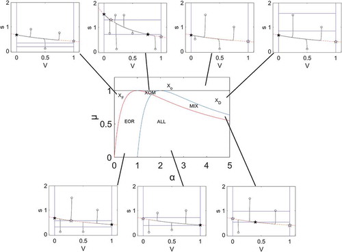
3.1 Collapse due to outside opportunities being too great (X₀)

When people have the opportunity to be better off outside the system (µ > 1), everyone leaves the system (Fig. 2, X₀). In these circumstances, the water availability condition does not play any role in determining the regime, and the CHWS collapses. On the other hand, when µ < 1, α comes into play in determining the regime. Different combinations of α and µ can result in six different regimes.

3.2 Collapse due to droughts (X_D)

The system can be under stress due to combinations of low inflow (moving the X_D regime boundary to the left of the phase diagram, e.g. Fig. 3(a)), high natural loss rate, and/or low extraction rate (perhaps owing to poor infrastructure (i.e. greater α, moving the system to the right of the phase diagram). In this case, if the payoff from working outside the system is sufficiently high (µ relatively high), the CHWS collapses (Fig. 2, X_D).

Figure 3. Effects of hydrological change on system regimes. Phase diagrams of the coupled human–water system (CHWS) under different hydrological conditions, superimposed on the contours of $V^{\ast }$: $V^{\ast }=0$ means the system collapses, while $V^{\ast }=1$ means that all stay. (a) 80% reduction in the inflow; (b) the baseline case (same as Fig. 2); and (c) 100% increase in the inflow

3.3 Collapse due to floods (X_F)

On the other hand, when inflow is too large (α too low), everyone again leaves the system, this time due to flood risks (Fig. 2, X_F).

3.4 Ideal (ALL)

Under “ideal” conditions – the system is threatened by neither droughts nor floods, and outside opportunities are not so lucrative – all stay and no one leaves the system (Fig. 2, ALL).

3.5 Either-or (EOR)

When the inflow is relatively high and the risk of flood increases but enough profit can still be made from working inside the system, the system experience bistability: the entire population would either stay or abandon the system, depending on its history (initial conditions) (Fig. 2, EOR). If a considerable proportion of the population stays, they would be extracting water, which in turn mitigates the flood risks; this makes the option of staying more attractive, providing incentives for more people to stay. On the other hand, if not enough people stay to begin with, the flood risk will remain high, discouraging other people from staying, and the system eventually collapses.

3.6 Mixed strategy (MIX)

On the other hand, when the inflow is relatively low and the water is scarce but enough profit can still be made from working inside the system, people allocate their efforts both inside and outside the system (Fig. 2, MIX). Here, if people extract too much water, each would receive less water and profit less, thereby incentivizing others to invest more efforts in working outside. If too many people work outside, there will be more water to share among the remaining people, allowing them to profit more, thereby incentivizing others to invest more effort working inside. These adjustments lead to a stable equilibrium where the payoffs of working inside and outside are equal.

3.7 Complex (XOM)

When the hydrological conditions are not too harsh and the outside opportunities are not too bad, the CHWS may either collapse (X) or see its population adopting mixed strategies (M) (hence, XOM), depending on the system’s history (initial conditions) (Fig. 2, XOM).

We also investigated how changes in hydrological conditions (e.g. climate change) affect these regime boundaries (Fig. 3). Not surprisingly, as inflow decreases, regime X_D expands while X_F shrinks (Fig. 3(a)); the opposite is true when inflow increases (Fig. 3(c)). The shape of regime ALL responds to these hydrological changes differently: it seems to be squeezed and skewed significantly under the reduced inflow scenario (Fig. 3(a)), while it appears to simply shift to the right with a minor change in shape (Fig. 3(c)).

The warped shape of regime MIX under the dry conditions (Fig. 3(a)) also tells a story of resilience against outside economic drivers. When the system’s natural loss rate is high and/or the water extraction rate is low (high α), a small improvement in outside opportunities (a small increase in µ) can push the system from ALL to X_D. For a CHWS with relatively low α, on the other hand, regime MIX – which can be seen as a buffer between regimes ALL and X_D – is wider, and it would take significantly greater improvement in outside opportunities to nudge the system from ALL all the way to X_D.

The model also has some implications for water management policies in a climate change context. The model results suggest that inappropriate water management (e.g. economic incentives affecting µ or water transfer projects affecting the regime boundaries as in Fig. 3) may trigger population displacement by moving a water system from one regime to another regime. For example, during the past few decades, the central plateau of Iran has seen a fast population growth due to urbanization and industrial and agricultural development (Gohari et al. 2013b). On top of this, crop production and water productivity of all crops have decreased considerably in the region due to lower precipitation and higher water requirements under higher temperature caused by climate change (higher water loss rate and thus higher α) (Gohari et al. 2013a). These changes pushed farmers to switch to less water-intensive crops (Boazar et al. 2019) and even caused land-use change (more profitable sectors – with higher µ) (Madani 2014). Here, $V^{\ast }$can be considered a proxy for people switching from a water-dependent sector/industry to a less water-sensitive one. To tackle this issue, a number of water transfer projects have been launched, thereby doubling the natural flow discharged into this region (Madani 2014). Despite all these measures, the water crisis has worsened in the last decade. In fact, the central plateau of Iran has been experiencing a severe hydrological and ecological regime shift, and the implemented water transfer policies have had a major role in accelerating this issue (Abrishamchi and Tajrishi 2005). Likewise, Madani (2014) concluded that these implemented water management policies have been inadequate and caused significant unintended side effects and suggested that the situation called for a comprehensive solution that simultaneously controls the dynamics of the system and minimizes the risk of unintended consequences. Indeed, insights about regime shifts and the phase diagram could provide a useful lens through which to view such intertwined dynamics.

With $V^{\ast }$ as a proxy for people who remain and $1-V^{\ast }$ a proxy for people who migrate, Fig. 3 also tells a story of migration response under environmental change. As the system becomes drier – imagine yourself located somewhere in regime ALL while the regime boundaries are shifting from Fig. 3(b) to Fig. 3(a) – your system will undergo a regime change from ALL to MIX to X_D. That is, people gradually adjust to the drier environment by migrating to find outside opportunities. The situation is different when the system becomes wetter (e.g. more flood-prone): it undergoes a regime change from ALL to EOR to X_F. In this case, while under regime EOR, $V^{\ast }$ is still at 1, but the alternative undesirable outcome already exists. Once the system crosses from EOR to X_F, one can expect to see an abrupt exodus of migrants, leaving the CHWS to collapse in a dramatic fashion.

4 Conclusions and final remarks

In this paper, we developed a 2D stylized model of a generic coupled human–water system (CHWS). Despite its simplicity, the model yielded a rich catalogue of seven different regimes, ranging from collapse due to a variety of causes to a regime where everyone is content with the system, and other distinct regimes in between. Our results suggest that sustainable management of a CHWS requires adequate knowledge of possible regimes to avoid a transition to undesirable ones. To this end, we examined how social and biophysical drivers (e.g. economic opportunities outside the system, hydrological conditions, and climate change) interact to determine the regime of a CHWS, clarifying how they interplay to define the regime boundaries. The model also eases the way to investigate the effects of social and hydrological drivers, individually and in combination, on regime shifts in CHWS. It contributes to better understanding of the nature of different regimes embedded in the coupled system and therefore the system’s resilience, which can potentially be useful in developing an early warning system for such socio-hydrological systems.

Exposing the modeled CHWS to environmental change (as in Fig. 3) sheds light on the nature of possible regime shifts and their implications on migration patterns. The results suggest there will be gradual migration in response to drier conditions and abrupt exodus in response to an increase in flood risk. Other “experiments” on how CHWSs may respond to changes in other drivers are possible: rapid population growth, agricultural and industrial development, new economic conditions, etc. These drivers influence the internal dynamics and feedback of CHWSs and can lead to regime shifts. Insights and intuition obtained from simple models like ours are useful in their own right and can play important parts in more sophisticated models of CHWS. In this way, our study has contributed to the body of knowledge on regime shifts specific to CHWSs and paved the way for further studies in this area.

Acknowledgements

MH and RM acknowledge support from the Army Research Office/Army Research Laboratory. The research reported in this article was supported by the Army Research Office/Army Research Laboratory under award no. W911NF1810267 (Multidisciplinary University Research Initiative – MURI). The views and conclusions contained in this document are those of the authors and should not be interpreted as representing the official policies either expressed or implied of the Army Research Office or the US Government.

Disclosure statement

No potential conflict of interest was reported by the authors.

Additional information

Funding

This work was supported by the Army Research Office/Army Research Laboratory [W911NF1810267].

Appendix

Here we elaborate on the determination of different regimes and the stability analysis that accompanies it. Figure A1 shows an example of the system phase plane with a few phase portraits.

Figure A1. An example phase plane of the system. The red and blue lines are the isoclines associated with the available water in the system (s) and the fraction of effort a user spends inside the system (V), respectively. The open circles indicate the initial points, the black curves emanating from them are the phase portraits, and the solid stars are the stable equilibrium points. The blue and red arrows show the direction of change in variables V and s. This particular example corresponds to regime XOM

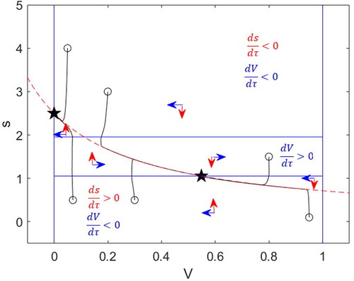
Graphically speaking, locating where the s-isocline (red) intersects with the V = 0 and V = 1 V–isoclines (blue) is useful in determining what regime the system is in: at $V^{\ast }=0,s^{\ast }=\frac{1}{\alpha }$ and at $V^{\ast }=1,s^{\ast }=\frac{1}{1+\alpha }$. The locations of $s^{\ast }=\frac{1}{\alpha }$ and $s^{\ast }=\frac{1}{1+\alpha }$ relative to the other two, horizontal, V–isoclines determine which of the seven regimes the system is in (see section 3). These considerations amount to the following expressions for the blue and red boundaries in Fig. 2, respectively:

(A1) $\begin{array}{c}\mu =C\left(\frac{1}{\alpha }-a\right)\left(b-\frac{1}{\alpha }\right)\\ \mu =C\left(\frac{1}{1+\alpha }-a\right)\left(b-\frac{1}{1+\alpha }\right)\end{array}$(A1)

We also determined the stability of each equilibrium point in each regime more formally by evaluating the signs of trace and determinant of the following Jacobian matrix at the equilibrium point of interest:

(A2) $J=\left[\begin{array}{cc}{J}_{11}& J_{12}\\ J_{21}& J_{22}\end{array}\right]=\left[\begin{array}{cc}-\left(V^{\ast }+\alpha \right)& -s^{\ast }\\ 2\beta C{V}^{\ast }\left(1-V^{\ast }\right)\left(\frac{a+b}{2}-s^{\ast }\right)& 2\beta \left(\frac{1}{2}-V^{\ast }\right)\left(U(s^{\ast }\right)-\mu )\end{array}\right]$(A2)

The Jacobian matrix was derived from the system of Equation (5)(5) $\begin{array}{c}\frac{ds}{d\tau }=1-Vs-\alpha s\\ \\ \frac{dV}{d\tau }=\beta V\left(1-V\right)\left(U-\mu \right)\end{array}$(5) . An equilibrium point is stable if its Jacobian matrix has negative trace and positive determinant. A few observations are useful for determining such stability. Note that J₁₁ < 0 and J₁₂ < 0. The sign of J₂₁ depends on the term $\left(a+b\right)/2-s^{\ast }$: J₂₁ > 0 if $s^{\ast }$is lower than the midpoint between the two thresholds of the utility function U(s). The sign of J₂₂ depends on the terms $\left(1/2-V^{\ast }\right)$ and $\left(U\left(s^{\ast }\right)-\mu \right):\left(1/2-V^{\ast }\right)>0$ if the majority of people (more than half) have migrated away from the system, while $\left(U\left(s^{\ast }\right)-\mu \right)>0$ if, at the equilibrium, the payoff of working inside the system is greater than working outside. The stability of each equilibrium point in each regime is summarized in Table A1.

Table A1. Mathematical expressions and stability of each equilibrium point in each regime. The solid and open circles signify stable and unstable equilibrium points, respectively

Regime	Stability	$V^{\ast }$	$s^{\ast }$
X	●	0	$1/\alpha$
	○	1	$1/\left(1+\alpha \right)$
${\mathrm{X}}_{\mathrm{D}}$	●	0	$1/\alpha$
	○	1	$1/\left(1+\alpha \right)$
${\mathrm{X}}_{\mathrm{F}}$	○	0	$1/\alpha$
	●	1	$1/\left(1+\alpha \right)$
ALL	○	0	$1/\alpha$
	●	1	$1/\left(1+\alpha \right)$
EOR	●	0	$1/\alpha$
	○	$\frac{1}{s^{\ast }}-\alpha$	$\frac{1}{2}\left(a+b+\sqrt{{\left(a-b\right)}^2+\frac{4\mu }{C}}\right)$
	●	1	$1/\left(1+\alpha \right)$
MIX	○	0	$1/\alpha$
	●	$\frac{1}{s^{\ast }}-\alpha$	$\frac{1}{2}\left(a+b-\sqrt{{\left(a-b\right)}^2+\frac{4\mu }{C}}\right)$
	○	1	$1/\left(1+\alpha \right)$
XOM	●	0	$1/\alpha$
	○	$\frac{1}{s^{\ast }}-\alpha$	$\frac{1}{2}\left(a+b-\sqrt{{\left(a-b\right)}^2+\frac{4\mu }{C}}\right)$
	●	1	$1/\left(1+\alpha \right)$
	○	$\frac{1}{s^{\ast }}-\alpha$	$\frac{1}{2}\left(a+b+\sqrt{{\left(a-b\right)}^2+\frac{4\mu }{C}}\right)$

References

- Abrishamchi, A. and Tajrishi, M., 2005. Interbasin water transfer in Iran. In: Water conservation, reuse, and recycling: proceeding of an Iranian American workshop. Washingon, DC: The National Academies Press, 252–271.
- Andersen, T., et al., 2009. Ecological thresholds and regime shifts: approaches to identification. Trends in Ecology & Evolution, 24 (1), 49–57. doi:https://doi.org/10.1016/j.tree.2008.07.014.
- Basok, T., 1993. Keeping heads above water: Salvadorean refugees in Costa Rica. Montreal: McGill-Queen’s Press-MQUP.
- Bauch, C.T., et al., 2016. Early warning signals of regime shifts in coupled human–environment systems. Proceedings of the National Academy of Sciences, 113 (51), 14560–14567. doi:https://doi.org/10.1073/pnas.1604978113.
- Biggs, R., Carpenter, S.R., and Brock, W.A., 2009. Turning back from the brink: detecting an impending regime shift in time to avert it. Proceedings of the National Academy of Sciences, 106 (3), 826–831. doi:https://doi.org/10.1073/pnas.0811729106.
- Biggs, R., Peterson, G.D., and Rocha, J.C., 2018. The regime shifts database: a framework for analyzing regime shifts in social-ecological systems.
- Black, R., et al., 2011. The effect of environmental change on human migration. Global Environmental Change, 21, S3–S11. doi:https://doi.org/10.1016/j.gloenvcha.2011.10.001
- Boazar, M., Yazdanpanah, M., and Abdeshahi, A., 2019. Response to water crisis: how do iranian farmers think about and intent in relation to switching from rice to less water-dependent crops? Journal of Hydrology, 570, 523–530. doi:https://doi.org/10.1016/j.jhydrol.2019.01.021
- Bonacci, O., Buzjak, N., and Roje-Bonacci, T., 2016. Changes in hydrological regime caused by human intervention in karst: the case of the rumin springs. Hydrological Sciences Journal, 61 (13), 2387–2398. doi:https://doi.org/10.1080/02626667.2015.1111518.
- Bury, T.M., Bauch, C.T., and Anand, M., 2019. Charting pathways to climate change mitigation in a coupled socio-climate model. PLoS Computational Biology, 15 (6), e1007000. doi:https://doi.org/10.1371/journal.pcbi.1007000.
- Carpenter, S.R. and Brock, W.A., 2006. Rising variance: a leading indicator of ecological transition. Ecology Letters, 9 (3), 311–318. doi:https://doi.org/10.1111/j.1461-0248.2005.00877.x.
- Carpenter, S.R. and Kinne, O., 2003. Regime shifts in lake ecosystems: pattern and variation. Vol. 15. Oldendorf/ Luhe, Germany: International Ecology Institute.
- Coutinho, R.M., Kraenkel, R.A., and Prado, P.I., 2015. Catastrophic regime shift in water reservoirs and São Paulo water supply crisis. PloS One, 10 (9), e0138278. doi:https://doi.org/10.1371/journal.pone.0138278.
- Cressman, R. and Tao, Y., 2014. The replicator equation and other game dynamics. Proceedings of the National Academy of Sciences, 111 (Supplement_3), 10810–10817. doi:https://doi.org/10.1073/pnas.1400823111.
- Deyoung, B., et al., 2008. Regime shifts in marine ecosystems: detection, prediction and management. Trends in Ecology & Evolution, 23 (7), 402–409. doi:https://doi.org/10.1016/j.tree.2008.03.008.
- Folke, C., et al., 2004. Regime shifts, resilience, and biodiversity in ecosystem management. Annual Review of Ecology, Evolution, and Systematics, 35 (1), 557–581. doi:https://doi.org/10.1146/annurev.ecolsys.35.021103.105711.
- Gohari, A., et al., 2013a. Climate change impacts on crop production in Iran’s Zayandeh-Rud River Basin. Science of the Total Environment, 442, 405–419. doi:https://doi.org/10.1016/j.scitotenv.2012.10.029
- Gohari, A., et al., 2013b. Water transfer as a solution to water shortage: a fix that can backfire. Journal of Hydrology, 491, 23–39.
- Gunderson, L., et al., 2017. Regime shifts and panarchies in regional scale social-ecological water systems. Ecology and Society: A Journal of Integrative Science for Resilience and Sustainability, 22 (1), 1. doi:https://doi.org/10.5751/ES-08879-220131.
- Haug, G.H., et al., 2003. Climate and the collapse of maya civilization. Science, 299 (5613), 1731–1735. doi:https://doi.org/10.1126/science.1080444.
- Hengl, S., et al., 2007. Data-based identifiability analysis of non-linear dynamical models. bioinformatics, 23 (19), 2612–2618. doi:https://doi.org/10.1093/bioinformatics/btm382.
- Hodell, D.A., Curtis, J.H., and Brenner, M., 1995. Possible role of climate in the collapse of classic maya civilization. Nature, 375 (6530), 391–394. doi:https://doi.org/10.1038/375391a0.
- Hofbauer, J. and Sigmund, K., 2003. Evolutionary game dynamics. Bulletin of the American Mathematical Society, 40 (4), 479–519. doi:https://doi.org/10.1090/S0273-0979-03-00988-1.
- Jägerskog, A. and Swain, A., 2016. Water, migration and how they are interlinked. Content.
- Jolliffe, I.T. and Cadima, J., 2016. Principal component analysis: a review and recent developments. Philosophical Transactions of the Royal Society A: Mathematical Physical and Engineering Sciences, 374 (2065), 20150202.
- Lade, S.J., et al., 2013. Regime shifts in a social-ecological system. Theoretical Ecology, 6 (3), 359–372. doi:https://doi.org/10.1007/s12080-013-0187-3.
- Lafuite, A.-S., De Mazancourt, C., and Loreau, M., 2017. Delayed behavioural shifts undermine the sustainability of social–ecological systems. Proceedings of the Royal Society B: Biological Sciences, 284 (1868), 20171192. doi:https://doi.org/10.1098/rspb.2017.1192.
- Madani, K., 2014. Water management in iran: what is causing the looming crisis? Journal of Environmental Studies and Sciences, 4 (4), 315–328. doi:https://doi.org/10.1007/s13412-014-0182-z.
- Mantua, N., 2004. Methods for detecting regime shifts in large marine ecosystems: a review with approaches applied to north pacific data. Progress in Oceanography, 60 (2–4), 165–182. doi:https://doi.org/10.1016/j.pocean.2004.02.016.
- Mittal, N., et al., 2016. Impact of human intervention and climate change on natural flow regime. Water Resources Management, 30 (2), 685–699. doi:https://doi.org/10.1007/s11269-015-1185-6.
- Montanari, A., et al., 2013. “panta rhei—everything flows”: change in hydrology and society—the iahs scientific decade 2013–2022. Hydrological Sciences Journal, 58 (6), 1256–1275. doi:https://doi.org/10.1080/02626667.2013.809088.
- Muneepeerakul, R. and Anderies, J.M., 2017. Strategic behaviors and governance challenges in social-ecological systems. Earth’s Future, 5 (8), 865–876. doi:https://doi.org/10.1002/2017EF000562.
- Muneepeerakul, R. and Anderies, J.M., 2020. The emergence and resilience of self-organized governance in coupled infrastructure systems. Proceedings of the National Academy of Sciences, 117 (9), 4617–4622. doi:https://doi.org/10.1073/pnas.1916169117.
- Muradian, R., 2001. Ecological thresholds: a survey. Ecological Economics, 38 (1), 7–24. doi:https://doi.org/10.1016/S0921-8009(01)00146-X.
- Nayak, P.K. and Armitage, D., 2018. Social-ecological regime shifts (sers) in coastal systems. Ocean & Coastal Management, 161, 84–95. doi:https://doi.org/10.1016/j.ocecoaman.2018.04.020
- Nowak, M.A., 2006. Evolutionary dynamics: exploring the equations of life. Cambridge: Harvard University Press.
- Querner, E., 2000. The effects of human intervention in the water regime. Ground Water, 38 (2), 167–171. doi:https://doi.org/10.1111/j.1745-6584.2000.tb00327.x.
- Rodionov, S., 2005. A brief overview of the regime shift detection methods. Large-scale disturbances (regime shifts) and recovery in aquatic ecosystems: challenges for management toward sustainability, 17–24.
- Rudnick, D.L. and Davis, R.E., 2003. Red noise and regime shifts. Deep Sea Research Part I: Oceanographic Research Papers, 50 (6), 691–699. doi:https://doi.org/10.1016/S0967-0637(03)00053-0.
- Scheffer, M., et al., 2001. Catastrophic shifts in ecosystems. Nature, 413 (6856), 591–596. doi:https://doi.org/10.1038/35098000.
- Schröder, A., Persson, L., and De Roos, A.M., 2005. Direct experimental evidence for alternative stable states: a review. Oikos, 110 (1), 3–19. doi:https://doi.org/10.1111/j.0030-1299.2005.13962.x.
- Schuster, P. and Sigmund, K., 1983. Replicator dynamics. Journal of Theoretical Biology, 100 (3), 533–538. doi:https://doi.org/10.1016/0022-5193(83)90445-9.
- Selby, J. and Hoffmann, C., 2012. Water scarcity, conflict, and migration: a comparative analysis and reappraisal. Environment and Planning C: Government and Policy, 30 (6), 997–1014. doi:https://doi.org/10.1068/c11335j.
- Sivapalan, M., Savenije, H.H., and Blöschl, G., 2012. Sociohydrology: a new science of people and water. Hydrological Processes, 26 (8), 1270–1276. doi:https://doi.org/10.1002/hyp.8426.
- Thompson, S., et al., 2013. Developing predictive insight into changing water systems: use-inspired hydrologic science for the anthropocene. Hydrology and Earth System Sciences, 17 (12), 5013–5039. doi:https://doi.org/10.5194/hess-17-5013-2013.
- Tilman, A.R., Watson, J.R., and Levin, S., 2017. Maintaining cooperation in social-ecological systems:. Theoretical Ecology, 10 (2), 155–165. doi:https://doi.org/10.1007/s12080-016-0318-8.
- Van De Meene, S., Brown, R.R., and Farrelly, M.A., 2011. Towards understanding governance for sustainable urban water management. Global Environmental Change, 21 (3), 1117–1127. doi:https://doi.org/10.1016/j.gloenvcha.2011.04.003.
- Wang, H., et al., 2017. Impacts of the dam-orientated water-sediment regulation scheme on the lower reaches and delta of the yellow river (huanghe): a review. Global and Planetary Change, 157, 93–113. doi:https://doi.org/10.1016/j.gloplacha.2017.08.005.
- Warziniack, T., 2013. The effects of water scarcity and natural resources on refugee migration. Society & Natural Resources, 26 (9), 1037–1049. doi:https://doi.org/10.1080/08941920.2013.779339.
- Yu, D.J., et al., 2014. The effect of infrastructure on social-ecological system dynamics: provision thresholds and asymmetric access.
- Zeileis, A., et al., 2003. Testing and dating of structural changes in practice. Computational Statistics & Data Analysis, 44 (1–2), 109–123. doi:https://doi.org/10.1016/S0167-9473(03)00030-6.