Long-term and event-scale sub-daily streamflow and sediment simulation in a small forested catchment

ABSTRACT

In small catchments, the time interval most commonly used for simulation – daily or monthly – may not be sufficient to accurately capture the time distribution of hydrological processes. In this paper, the Soil and Water Assessment Tool (SWAT) was used to perform an hourly long-term streamflow and sediment load simulation in the small (4.8 km²) and forested Aixola catchment (northern Spain). From this simulation, 10 runoff events were tested; the most satisfactory results for streamflow were obtained under wet antecedent conditions. However, simulated sediment load was underestimated during the peaks and remained high towards the end of the event. Furthermore, the influence of the precipitation time step (1–4 h, daily) was not relevant in the streamflow simulation but does influence the sediment simulation. The best results were achieved with the daily step simulations obtained at an hourly time step. This paper shows that sub-daily modelling improves water and especially sediment yield results; however, improvements are still needed in timing-related routines.

KEYWORDS:

• sub-daily simulation
• long-term
• runoff events
• suspended sediments
• antecedent conditions
• high-resolution data

Editor A. Castellarin ; Associate editor J. Rodrigo-Comino

1 Introduction

Headwater catchments provide a relevant proportion of streamflow to many fluvial systems (Cartwright et al. 2018). They also have a significant influence on the quality and quantity of water that is eventually used downstream for agriculture, industry, and human consumption (Freeman et al. 2007). Therefore, studying the hydrological processes in headwater areas is relevant for assessing catchment management practices. On the other hand, the hydrological processes generate sediment that contribute significantly to global sediment delivery (Kao and Milliman 2008). However, an increase in fine sediment can harm aquatic life (Rymszewicz et al. 2018) and can be an important vector for the transport of nutrients and contaminants such as heavy metals (Garmendia et al. 2019), pesticides (Boithias et al. 2014), and microorganisms (Kim et al. 2017). Hence, it is necessary to study the sediment dynamics of fluvial systems as it can play an important role in water quality. Such analyses could help guide the Water Framework Directive (WFD; 2000/60/EC) – particularly, as Förstner (2015) suggests, “the Directive neglects the role of sediments as a long-term secondary source of contaminants. Such a lack of information may easily lead to unreliable risk analyses with respect to the – pretended – ‘good status.’” Thus, studying the suspended sediment dynamics can provide information about the geomorphological and ecological status of the fluvial systems and helps in the assessment of soil erosion in headwater catchments.

Catchment managers together with other stakeholders may implement water protection measures, possibly based on modelling results conducted by research institutes. However, the commonly performed monthly or daily catchment modelling may not be sufficient for any purpose as it does not capture the intensity of precipitation. Thus, modelling catchments with rapid response at daily or monthly time steps is not enough to study hydrological processes that may occur at sub-daily time scales. Many models are capable of performing simulations of storm events at a sub-daily time step, e.g. ANSWERS (Areal Nonpoint Source Watershed En-vironment Response Simulation) (Park et al. 1982) or EUROSEM (European Soil Erosion Model) (Morgan et al. 1998). The modelling of storm events is important to understand the hydrological processes at the catchment scale and to analyse and predict runoff generation or evaluate contaminant/nutrient delivery, among other things. Few models can both simulate single events and perform long-term continuous simulation at a sub-daily time step.

Since 2010, the code of the Soil and Water Assessment Tool (SWAT) (Arnold et al. 1998) has been modified with physically based algorithms to improve the simulation of streamflow (Jeong et al. 2010), erosion, and suspended sediment transport (Jeong et al. 2011) at the sub-daily scale. It is expected that in the near future, SWAT+ will undergo continuous improvements including some sub-daily algorithms (Bieger et al. 2016). Thus, it is possible to perform long-term continuous simulations and analyse single runoff events (including discharge, sediments, and nutrients) in quick-response small headwater catchments that require sub-daily modelling. This duality affords the ability to understand the hydrological processes while considering the long-term impacts.

The sub-daily option of the SWAT model has already been used in small urbanised or agricultural areas (e.g. Kannan et al. 2007, Jeong et al. 2014, Bauwe et al. 2017) and, more rarely, in large catchments (e.g. Yang et al. 2016, Boithias et al. 2017, Yu et al. 2018). Regarding sediment simulation, Jeong et al. (2011) and Furl et al. (2015) evaluated the sub-daily sediment transport in small agricultural catchments, while Kaffas et al. (2018) modelled continuous hydromorphological processes in a large mountainous basin. In general, these studies have had good results; however, in many of them sub-daily modelling was used to evaluate the daily streamflow (e.g. Kannan et al. 2007, Maharjan et al. 2013, Furl et al. 2015, Yang et al. 2016) and in most of them the sediment load was modelled in very small (<1 km) experimental catchments. Nevertheless, the capability of SWAT models to simulate at a sub-daily time step streamflow and sediment transport in a small and forested headwater catchment has never been tested.

In a recent review of papers in which SWAT was used at a sub-daily time step, Brighenti et al. (2019) identified some of the shortcomings and possible ways forward in simulating sub-daily processes with the model. They deduced that the detailed understanding of the model’s sub-daily application remains limited. However, some conclusions were made concerning (among other issues) the methods to simulate infiltration, the suitable time step for sub-daily modelling, and the consideration of the temporal structure of precipitation. Finally, they emphasised that the main challenge in using the sub-daily routines is the lack of high-resolution data that could be used to improve the calibration and validation processes.

The present study evaluated the SWAT model’s sub-daily performance in a forested headwater catchment of the Basque Country (Atlantic watershed of the Iberian Peninsula), where the river drains into a reservoir that is used for water supply (Fig. 1). Long-term continuous streamflow and sediment transport were simulated using SWAT, and then different runoff events were analysed. The model has already been used in this catchment at a daily time step to evaluate the impacts of climate change on runoff and sediment yield (Zabaleta et al. 2014), and to analyse its performance on simulating the spatial origin of the streamflow (Meaurio et al. 2015). Nevertheless, due to the quick response of the catchment to precipitation (Zabaleta et al. 2007, Zabaleta and Antigüedad 2013), the simulated streamflow peaks, and consequently the sediment peaks, were underestimated. We hypothesised that the sub-daily option of SWAT would allow for better streamflow and sediment simulations.

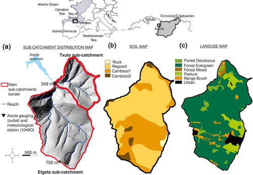
Figure 1. Location of Aixola catchment and (a) hillshade with sub-catchment distribution map (Elgeta and Txulo), (b) soil map and (c) land-use map

The main objective of this study was to evaluate the performance of the SWAT model in simulating streamflow and suspended sediment at a sub-daily time step in a small and forested headwater catchment. Hence, the model was carried out using hourly precipitation input, and the performance was evaluated following these steps: (1) perform a long-term continuous modelling to calibrate and validate the streamflow at an hourly time step and sediments at hourly and daily time steps; (2) compare the hourly simulation results at a daily time step; (3) change the hourly precipitation to 2, 3 and 4 h to evaluate the influence of precipitation input time step in the simulation results; and (4) evaluate the hourly simulation performance for single runoff events. This research could help SWAT users, and therefore managers, to decide which time step is better depending on their objectives.

2 Materials and methods

2.1 Study area

The Aixola catchment is located at coordinates 540513, 4777147 (UTM 30N ETRS89; in the central part of the Basque Country) in the Atlantic watershed of the Iberian Peninsula (Fig. 1). It is a small catchment (4.6 km²) that can be divided into two main sub-catchments, Txulo at 1.1 km² and Elgeta at 3.5 km² (Fig. 1(a)). The river drains into the Aixola reservoir (2.73 hm³), and its water is used for drinking water supply (for 27 530 inhabitants).

The elevation of the catchment ranges from 340 m in the gauging station to 750 m at the highest peak (Fig. 1(a)). Therefore, the slopes in the catchment are significant, but they do not usually exceed 30%. The main soils are deep (1–13 m) cambisols and regosols (IUSS-WRB 2015) with a loamy texture (Fig. 1(b)). The characteristics of these soils (depth, texture, organic matter, hydraulic conductivity, available water capacity, bulk density) are known thanks to soil samples obtained in 2012 (Meaurio et al. 2015). The lithology in 94% of the catchment is the practically impervious Upper Cretaceous calcareous flysch. Aixola is a highly forested catchment, and Pinus radiata plantations cover 80% of the total area (Fig. 1(c)).

The gauging and meteorological stations are located at the entrance of the reservoir (Fig. 1(a)). Since 1986, the meteorological station has measured precipitation and air temperature every 10 min. The streamflow has been measured since 1991 and the turbidity (NTU) since 2003, both of them measured every 10 min. The measured turbidity is used to estimate the suspended sediment yield (Zabaleta et al. 2007). Since 2011, the electrical conductivity (at 25°C, hereafter EC, µS cm⁻¹) of water is measured every 20 min, and its value is used to separate the baseflow (BF) and the surface runoff (SR) using the conductivity mass balance approach (CMB) (Stewart et al. 2007), which has previously been used in this catchment (Zabaleta and Antigüedad 2013, Meaurio et al. 2015). The climate is humid and temperate. From 2005 to 2014, the mean annual precipitation was 1450 mm, the mean annual temperature was 12°C, the mean annual streamflow was 0.093 m³ s⁻¹ (around 600 mm y⁻¹), and the mean suspended sediment concentration of water was 14.1 mg L⁻¹.

2.2 SWAT model

The Soil and Water Assessment Tool (SWAT) is a semi-distributed hydrological and environmental model that considers the catchment scale; in addition, it can simulate continuously in time. The Agricultural Research Service of the US Department of Agriculture (USDA) developed this model to predict the effect of land management practices on water, sediments, and agricultural chemical yields (Arnold et al. 1998). SWAT2012 is capable of conducting long-term continuous- and single-event-scale hydrological simulations at catchment scale to simulate hydrological processes (Jeong et al. 2010), soil erosion, and sediment transport and deposition (Jeong et al. 2011).

SWAT considers the catchment hydrology in two major phases. The first phase is the land phase, which controls all the processes occurring in the hydrological response units (HRU; catchment division with homogeneous land use, soil, and slope) before water, sediments, and nutrients enter into the channel network. The second phase is the routing phase of the hydrologic cycle, which considers the movement of water, sediments, and nutrients through the channel network up to the catchment outlet. Table 1 shows the main methods used by the model at daily and sub-daily time steps. In general terms, the sub-daily modelling is performed with physically based equations. One of the most important differences between the daily and the sub-daily modelling is the way in which the infiltration and the surface runoff are calculated. At the daily time step, the empirical Soil Conservation Service Curve Number Method (SCS CN; Soil Conservation Service, USDA 1972) is used, while at a sub-daily time step the SWAT applies the physically based Green-Ampt Mein-Larson Method (GAML) (Mein and Larson 1973). All details on the daily SWAT modelling are explained by Neitsch et al. (2011), and details on SWAT sub-daily modelling are explained by Jeong et al. (2010, 2011).

Table 1. Main differences in the daily and sub-daily streamflow and sediment simulation methods in SWAT

		Streamflow		Sediment
Land phase	Daily	Infiltration and surface runoff	SCS CN method: CN is updated daily according to antecedent soil conditions, hydrological group, and slope (Soil Conservation Service, USDA 1972).	Soil loss	MUSLE equation: the empirical equation was modified to consider the runoff factor (Williams 1975).
	Sub-daily		Green and Ampt Mein Larson method: allows a continuous simulation of infiltration processes. Needs sub-daily precipitation as input (Mein and Larson 1973).		Splash erosion, which is important at sub-daily time step (canopy interception). Surface runoff routing: generates erosion (see Jeong et al. 2011).
Routing phase	Daily	Flow routing	Manning’s equation: calculates volumetric rate and velocity of the water (Manning 1891).	Routing: degradation and deposition	Bagnold (1977), Kodoatie (2000), Molinas and Wu (2001), Yang (1996).
	Sub-daily		Unit Hydrograph method: used to route the surface runoff each time step (SCS 1972).		Bagnold (1977), Yang (1996), Brownlie (1982).

For the sub-daily modelling, not all processes are modelled at a sub-daily time step; the surface runoff and streamflow routing phase are routed at a sub-daily time step but baseflow and evapotranspiration are calculated on a daily basis and distributed for each time step.

2.2.1 Modelling design: calibration, validation, and evaluation

The main inputs needed to perform the modelling project with ArcSWAT 2012 are the topography, the land use and the soil maps, and the meteorological data. In this study, the source for the three maps (the digital elevation model and the land-use and soil maps) was the Basque Government’s geographical database (www.geo.euskadi.eus). The meteorological data were obtained from the Gipuzkoa Provincial Council (www.gipuzkoa.eus/en/web/council). Below is a summary of the inputs:

1. Digital elevation model (5 m × 5 m) obtained using LIDAR data (2008).

2. Land-use classification (1:10 000) conducted in 2005.

3. Soil map (1:25 000). This map was modified to improve its accuracy, considering soil depth and texture obtained from boreholes and surficial sampling (Meaurio et al. 2015).

4. Hourly precipitation and maximum and minimum temperature from 1 January 2005 to 13 December 2014, as measured by the gauging station.

All details on the streamflow calibration in Aixola catchment at the daily time step are available in Meaurio et al. (2015), and the daily suspended sediment load, as well as the sub-daily streamflow and suspended sediment load, was calibrated during the present study. The hourly streamflow (m³ s⁻¹) and the sediment load (kg; obtained from turbidity measured at Aixola gauging station (following Zabaleta et al. 2007, 2014) were used to calibrate (from 2010 to 2014) and validate (from 2005 to 2009) the sub-daily model and the daily suspended sediment load (kg).

The calibration process at the sub-daily (hourly) time step was divided into the following steps:

Step 1. The calibration and validation periods were selected. The observed data included wet, average, and dry years, chosen to be representative of the hydrological processes that occur in the catchment.

Step 2. A one-at-a-time sensitivity analysis was performed with the SWAT Calibration and Uncertainty Program (SWAT-CUP; Abbaspour et al. 2007), as modified by Bressiani (2016) for a sub-daily time step.

Step 3. A preliminary manual calibration of the most sensitive parameters was conducted to identify the reasonable value range for each parameter. In addition, thanks to previous knowledge of the catchment and the availability of previous modelling studies (Zabaleta et al. 2014, Meaurio et al. 2015), other parameters were also calibrated. Once the value ranges were determined, they were introduced into the SWAT CUP program to adjust their values with the SUFI2 algorithm (Abbaspour et al. 2004, 2007), which is the most frequently used tool for model calibration in SWAT (Brighenti et al. 2019).

Step 4. The hourly simulation results (streamflow and sediment load) were compared graphically with those observed in the catchment and evaluated with statistical indices. The statistical indices used to evaluate the performance of the simulation were Nash-Sutcliffe efficiency (NSE; Nash and Sutcliffe 1970), the coefficient of determination (R²), the percent bias (PBIAS) (Gupta et al. 1999), and the standard deviation ratio (RSR) (Moriasi et al. 2007).

2.3 Evaluation of precipitation time step

The temporal resolution of precipitation inputs has a significant impact on sub-daily simulation results (Brighenti et al. 2019). Once the model was calibrated and validated at the hourly time step, other precipitation input steps (2, 3, and 4 h) were applied to the simulations to evaluate the influence of the precipitation time step in the streamflow and suspended sediment simulation. Simulation results were also compared with those obtained from daily time-step modelling. However, it is necessary to take into consideration the fact that the most important equations in the streamflow and suspended sediment simulation are different at daily and sub-daily time steps (Table 1), and therefore, the calibrations differ.

2.4 Selection of runoff events

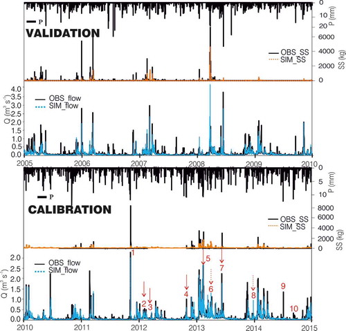
Ten runoff events registered in the calibration period (from 2010 to 2014; Fig. 2) were analysed to evaluate the SWAT simulation performance of different types of events. The sediment data from March to November 2012 are missing and, consequently, no runoff events were analysed for this period. In addition, all the events were selected from 2012–2014 because during this period, the EC was measured at the Aixola gauging station (Fig. 1(a)), allowing for the estimation of the BF/SR ratio.

Figure 2. Graphical results for the hourly streamflow (Q, L s⁻¹) and suspended sediment load (SS, kg) calibration (image below) and validation (top image). Precipitation (P, mm) of the period is included. The analysed event numbers and their performance are displayed in the calibration image; when the arrow is continuous the performance is at least satisfactory (both R² and RSR), when the arrow is discontinuous the performance is at least satisfactory (R² or RSR), and when there is no arrow the performance is unsatisfactory

The selected events represent different hydrological situations, antecedent conditions, rainfall intensity, and/or streamflow amount. The beginning of each event was established at the start of surface runoff, and the end was indicated by the depletion of all the surface runoff. In events with multiple peaks, the total depletion of surface runoff is not reached and peaks are considered collectively as a single event.

Five groups of parameters were considered in event characterization: (1) the conditions before the event; (2) the precipitation that generated the event; (3) the streamflow during the event; (4) SR and BF during the event; and (5) the suspended sediments delivered during the event.

1. To define the conditions before the event, the following parameters were considered: the precipitation 1 h before the event (bP1, mm) and 7 and 21 d before the event (bP7d, mm; bP21d, mm), and the mean streamflow measured in the gauging station 24 h before the event (bQ1d, L s⁻¹).

2. The precipitation that generated the event was analysed in terms of the mean intensity (IP, mm h⁻¹) and maximum intensity (IPmax, mm h⁻¹) of the rainfall.

3. The streamflow during the storm event was expressed as the mean streamflow measured at the gauging station (Qmean, L s⁻¹) and the ratio of the maximum streamflow to the streamflow before the event (Qmax/Qb).

4. With the EC data, a CMB approach was used to separate SR and BF (Meaurio et al. 2015). These were considered at a daily time step (starting at 0:00 and ending at 23:59) and expressed as the BF/SR ratio. These data were used to evaluate the simulated BF/SR distribution for the different storm events at a daily time step because, although the streamflow simulation was done sub-daily, SWAT calculates the BF/SR distribution daily.

5. The mean suspended sediment concentration (SSCmean, mg L⁻¹) and the total suspended sediment load (SST, kg) were also considered.

All these parameters (except those related to precipitation, as they are input data) were calculated for both observed and simulated values.

3 Results and discussion

3.1 Long-term continuous modelling; calibration and validation

Before conducting the hourly calibration, the most sensitive parameters for streamflow and suspended sediments were identified using SWAT CUP’s one-at-a-time sensitivity analysis (modified by Bressiani (2016) for sub-daily time step; see parameters marked with an asterisk in Table 2). The sensitivity analysis was carried out by varying each parameter within the assigned range while keeping the remaining parameters constant at realistic values. Thus, we started the calibration with the most sensitive parameters.

Table 2. SWAT parameters selected for hourly calibration: their description and calibration range, and the modifications carried out during calibration for each of the sub-catchments

	Change type	Parameter name	Description	Range	Txulo	Elgeta
Flow	v	*MSK_CO1.bsn	Calibration coefficient in Muskingum method	5–6	5.8
	v	*MSK_CO2.bsn	Calibration coefficient in Muskingum method	5–6	5.78
	v	*MSK_X.bsn	Weighting factor in Muskingum method	0.18–0.3	0.18
	v	*CNCOEF.bsn	Plant ET curve number coefficient	1–2	1.75
	v	ESCO.bsn	Soil evaporation compensation factor	0.7–0.9	0.9
	v	SURLAG.bsn	Surface runoff lag coefficient	0–5	1
	v	SFTMP.bsn	Snowfall temperature (°C)	0–5	1.1
	v	SMTMP.bsn	Snow melt base temperature (°C)	0–5	4.5
	v	*ALPHA_BF.gw	Baseflow alpha factor	0–0.3	0.005
	v	*GW_REVAP.gw	Groundwater “revap” coefficient	0–0.5	0.05	0.15
	v	GW_DELAY.gw	Groundwater delay time	0–500	450
	v	SHALLST.gw	Initial depth of water in the shallow aquifer	0–5000	1000
	v	GWQMN.gw	Threshold depth of water in shallow aquifer required for return flow to occur	0–1000	700
	v	DEEPST.gw	Initial depth of water in the deep aquifer	0–0.5	0
	v	RCHR_DP.gw	Deep aquifer percolation factor		0
	v	*CH_N2.rte	Manning’s nfor the main channel	0–2	0.023	0.152
	v	*CH_K2.rte	Main channel conductivity	0–50	42.07	15.79
	v	*CANMX.hru	Maximum canopy storage	0–2	0.07
	v	*LAT_TTIME.hru	Lateral flow travel time	0–5	3.918
	v	OV_N.hru	Manning’s n for overland flow	0–0.5	0.3
	r	ELEV. sub	Elevation at the centre of the elevation band		450	19
	r	ELEV_FR. sub	Fraction of sub-basin area within the elevation band		1	12
Sediment	v	*C_FACTOR.bsn	Cover and management factor for overland flow erosion	0.001–0.45	0.001
	v	*EROS_EXPO.bsn	Exponential coefficient for overland flow	0.5–2	0.55
	v	*CH_D50.bsn	Median particle diameter of main channel (mm)	0.5–20	0.75
	v	*RILL_MULTL.bsn	Rill erosion coefficient	0.5–1	0.55
	v	*ADJ_PKR.bsn	Peak rate adjustment factor for sediment routing	0.5–2	0.61
	r	*SPCON.bsn	Channel sediment routing parameter	0.001–0.01	0.01
	v	*SPEXP.bsn	Exponent parameter for calculating sediment re-entrained in channel	1–1.5	1.5
	v	*CANMX.hru	Maximum canopy storage	0–2	0.07
	v	*EROS_SPL.bsn	Splash erosion coefficient	0.9–1.5	1.09

Parameters marked with * were included in the sensitivity analysis.

v indicates that the default parameter is replaced by a given value, and r means the existing parameter value is changed relatively.

Considering the knowledge from previous modelling research works in the catchment (Zabaleta et al. 2014, Meaurio et al. 2015), other parameters were also included in the calibration (see Table 2) – for example, the parameters related to the deep aquifer. Taking into account the hydrological processes studied in these works and the geology of the catchment, it is possible to conclude that there is not a deep aquifer in Aixola. Therefore, the value for the parameters related with the deep aquifer (RCH_DP and DEEPST) is 0. Other examples are the elevation bands. There is an important elevation gradient in the catchment (from 349 m in the outlet to 750 m in the highest mountain, see Fig. 1); hence, ELEV and ELEV_FR are introduced in the present study. The potential evapotranspiration was calculated using the Hargreaves method (Hargreaves and Samani 1985). The most sensitive parameters with respect to calibrating streamflow were the ones that were related to the Muskingum routing method (Overton 1966) and the CNCOEF, which is the weighting coefficient used to calculate the retention coefficient for daily curve number calculations dependent on plant evapotranspiration. The values for these parameters were adjusted with the SUFI2 algorithm in the SWAT CUP program and are presented in Table 2. The calibration was made considering the long-term simulation but also the event-scale and some hydrological processes (baseflow/surface runoff), which made it more complex. For example, although the snow events are sporadic in the catchment, the parameters SFTMP (snowfall temperature (ºC)) and SMTMP (snow melt base temperature (ºC)) were calibrated because it was considered that they could exert an influence on some of the events (to simulate the delay of the streamflow and sediments).

The most sensitive parameters while calibrating sediments were the exponential coefficient for overland flow (EROS_EXPO), the median particle diameter (CH_D50), the scaling parameter for cover, and the management factor for overland flow erosion (C_FACTOR). In general, all changes were made with the aim of increasing the sediment amount, as the simulated sediment was considerably lower than the observed amount. Among these three parameters, the C_FACTOR was the most sensitive because of its high influence on soil erosion and therefore on the availability of sediment. The influence of the other sensitive parameters was low compared to the C_FACTOR. To increase the sediment simulation performance in peaks, the peak rate adjustment factor for sediment routing (ADJ_PKR) was calibrated. However, the influence of this parameter was limited. The rill erosion coefficient (RILL_MULT) was also increased, with the aim of increasing the suspended sediment content in the stream. Although the sensitivity of this parameter is high, it should be varied carefully because it generates many fluctuations. The other modified parameters were the channel sediment routing parameter (SPCON), exponent parameter for calculating sediment retrain in channel (SPEXP), and geometric standard deviation of particle size (SIG_G). The influence of these parameters on the performance of the sediment simulation was not significant, although their calibration marginally improved the results. Finally, the parameter SUBD_CHSED was changed to adjust to the catchment properties because this parameter provides three options for the instream sediment routing model. In this case, the second model (the Yang model) was selected as it is most appropriate for small catchments (Yang 1996).

Parameters such as maximum plant canopy storage (CANMX) influence streamflow and sediment simulation because increasing them decreases the amount of water that reaches the soil, and therefore, less sediment is generated. All the calibrated parameters and their values are shown in Table 2.

The statistical indices for the hourly calibration (from 2010 to 2014) show that the streamflow simulation could be classified as good (Table 3). For the validation period (from 2005 to 2009), NSE and RSR were satisfactory. As these statistical indices are very sensitive to extreme values, the peaks may fit better in the calibration period than in the validation period. This may be because during the validation period, the precipitation intensity of some events was higher than that in the calibration period and therefore, the streamflow peaks were also higher (Fig. 2). On the other hand, PBIAS and R² values showed that the streamflow calibration and validation were very good.

Table 3. Sub-daily and daily statistics obtained for calibration and validation of streamflow and suspended sediment simulations. According to Moriasi et al. (2015), the simulations are “satisfactory” at a daily time step when R² > 0.60, NSE > 0.50, RSR ≤ 0.70, and PBIAS ≤ ±15% for streamflow and R² > 0.40, NSE > 0.45, RSR ≤ 0.70, and PBIAS ≤ ±20% for sediment. Generally, as the evaluation time step decreases, a stricter performance rating is warranted (Moriasi et al. 2007). Bold formatting indicates results that are at least satisfactory

Statistical index	Calibration (2010–2014)				Validation (2005–2009)
	Hourly flow	Daily flow	Hourly sediment	Daily sediment	Hourly flow	Daily flow	Hourly sediment	Daily sediment
NSE	0.71	0.79	0.24	0.37	0.55	0.65	0.3	0.72
R^2	0.85	0.9	0.5	0.59	0.79	0.85	0.7	0.82
PBIAS	−12	−12	−0.22	−23	6	6	11	9
RSR	0.54	0.46	0.87	0.79	0.66	0.59	0.83	0.53

The sediment load hourly simulation performance (Fig. 2) showed that the magnitude of the simulated peaks was considerably lower than the observed values, i.e. the simulation did not generate as much sediment as that generated (in the Aixola catchment) in an actual event. Thus, NSE and RSR were unsatisfactory. The statistical indices were better for the validation period than for the calibration period. This is because in November 2011 (calibration), there was an extraordinary flood event that transported a large amount of sediment (~8000 kg) which was not simulated by the model. This had a significant impact on the statistical indices (Figs 2, 3(a)).

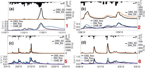
Figure 3. Graphical results for the hourly streamflow (bottom) and suspended sediment load (top) for events 1, 2, 5, and 6

OBS_flow is the observed streamflow, SIM_flow is the simulated streamflow, CMB_BF is the baseflow calculated with the conductivity mass valance approach, OBS_SS is the observed sediment load and the SIM_SS the simulated sediment load.

The statistical index values used to evaluate the simulation performance were initially established for monthly or daily simulation, and generally, as the evaluation time step decreases, a stricter performance rating is warranted (Moriasi et al. 2007).

In the daily sediment modelling, we modified the calibration parameters reported by Arnold et al. (2012). The parameters that were more heavily influenced were the USLE (Universal Soil Loss Equation) equation support particle factor (USLE_P, calibration value 0.7), the channel sediment routing parameter (SPCON, calibration value 0.0001), and the exponent parameter for calculating sediment re-entrained in channel (SPEXP, calibration value 1.5). The daily sediment modelling was conducted to evaluate the precipitation input influence. The results are discussed in section 3.3 (Table 4, 1D).

Table 4. Summary statistics obtained for NSE, R², PBIAS and RSR for simulations performed for the period 2005–2014 with 1, 2, 3, and 4 h and daily precipitation input. Daily statistics are included for simulation performed with 1 h precipitation (1d (hourly input)) and for simulation performed with daily precipitation data (1 d (daily input)). Bold formatting indicates results that are at least satisfactory

	NSE	R^2	PBIAS	RSR
Flow
1 h	0.71	0.89	−2.29	0.54
2 h	0.64	0.86	0.85	0.82
3 h	0.64	0.85	−12	0.71
4 h	0.64	0.82	−14	0.68
1 d (hourly input)	0.73	0.87	−3.2	0.52
1 d (daily input)	0.72	0.91	−9.7	0.53
Sediment
1 h	0.48	0.63	6	0.76
2 h	0.43	0.68	17	0.75
3 h	0.43	0.7	44	0.71
4 h	0.41	0.64	49	0.71
1 d (hourly input)	0.63	0.85	8.79	0.6
1 d (daily input)	0.54	0.89	−121.45	0.68

3.1.1 Evaluation of hourly simulation results at a daily time step

To evaluate whether the hourly simulation increased the daily performance, the statistical indices were calculated at a daily time step. As shown in Table 3, when the hourly streamflow performance was evaluated at a daily time step, the statistical indices improved. In general, the simulated and observed streamflow peaks fit better (for both NSE and RSR) and the PBIAS is lower, although with a minor improvement.

With respect to sediments, the Aixola catchment showed an immediate and significant response to storm events (Zabaleta et al. 2007, 2014). However, the simulation did not show an immediate response. Thus, the sediment load, instead of mainly concentrating during the event, was delivered over time (Fig. 3). An improvement in hourly modelling was observed when the simulated sediment load accumulated in 1 d, and these data fit much better with the daily observed values. Thus, the improvement in simulation was significant when the sediment simulated at a sub-daily time step was considered for the daily time step (Table 3).

3.1.2 Precipitation time-step influence in the modelling

Table 4 presents the summary statistics for the streamflow and suspended sediment simulation performed with different precipitation time steps. In sub-daily streamflow modelling, the statistical indices were marginally poor when the input precipitation time step increased (from 1 to 4 h). Nevertheless, the results for daily precipitation input were marginally poorer than those obtained with the hourly precipitation input (note that the simulation time step is also daily and the equations are different; see Table 1). Therefore, the precipitation time step had no significant effect on the streamflow simulation results.

The most significant differences with the observed data were found while simulating suspended sediment. The PBIAS statistical indices (Table 4) show that the sediment load was underestimated as the time step increased. The results were good for simulation of 1 and 2 h, whereas the results were unsatisfactory for simulation of 3 and 4 h. As the daily simulation was performed with daily precipitation data, although the statistical indices NSE, R², and RSR showed satisfactory results, the PBIAS indicates that the simulated sediment load was considerably underestimated. Therefore, the distribution of the precipitation throughout the day (precipitation intensity) is important in sediment modelling as it accounts for the suspended sediment dynamics in the catchment (Zabaleta et al. 2007, 2014). The best results for the daily statistical indices were obtained from hourly modelling, where all the indices showed at least satisfactory results.

Overall, the results show that in the Aixola catchment, it is possible to obtain good results for the streamflow with sub-daily and daily precipitation input and simulations. This outcome did not fully coincide with the conclusions reached by Maharjan et al. (2013) and Bauwe et al. (2017), who indicated that the best time scale for sub-daily modelling of streamflow with SWAT is 1 h. Nevertheless, in the Aixola catchment, the precipitation time step is important to obtain good results in sediment modelling, as results improved when the input precipitation time step decreased (e.g. Jeong et al. 2011, Yang et al. 2016). In this case, the best results for the daily statistical indices were obtained from hourly modelling, indicating that when the precipitation intensity is considered, although the total sediment amount was similar to the observed value, its transport timing could not be accurately simulated.

3.1.3 Analysis of the model performance during different types of events

After evaluating the long-term sub-daily simulation, the performance of SWAT was analysed for (1) dry antecedent moisture conditions and high precipitation intensity; (2) wet antecedent moisture conditions and moderate precipitation; and (3) events that did not belong to the first two groups. Ten storm events from the calibration period were selected for the evaluation. The events are numbered in the bottom image of Fig. 2.

The event characteristics for precipitation, streamflow, and suspended sediments are shown in Table 5. The observed and simulated sediment load (kg) and the observed and simulated streamflow (L s⁻¹) are presented, and in both cases, the RSR and R² results for each event are calculated. NSE and PBIAS were not used for the event performance evaluation because these statistical indices are not adequate for single events (Moriasi et al. 2015). Figure 3 shows the graphical results for different types of events that have been grouped considering similar characteristics.

Table 5. Characteristics of observed (OBS) and simulated (SIM) runoff events and statistical results (R² and RSR) of the simulated streamflow (FLOW) and suspended sediment load (SS). bP21d is the precipitation 21 d before the event, bP7d the precipitation 7 d before the event, and bP1 the precipitation 1 d before the event. OBSbQ1d is the observed streamflow 1 d before the event, IP is the mean intensity of the precipitation that generates the event, and Pmax is the maximum. Qmean is the mean streamflow during the event, Qmax/Qb is the ratio of the maximum streamflow to the streamflow before the event, and BF/SR is the ratio of the baseflow to the surface runoff. SSCmean is the mean suspended sediment concentration and SST is the total suspended sediment load. Bold formatting indicates results that are at least satisfactory

Event	Date	bP21d (mm)	bP7d (mm)	bP1 (mm)	OBS bQ1d (L s^−1)	IP (mm h^−1)	IPmax (mm h^−1)	OBS Qmean (L s^−1)	SIM Qmean (L s^−1)	OBS Qmax/Qb	SIM Qmax/Qb	OBS BF/SR	SIM BF/SR	FLOW RSR	FLOW R^2	OBS SSCmean (mg L^−1)	SIM SSCmean (mg L^−1)	OBS SST (kg)	SIM SST (kg)	SS RSR	SS R^2
1	4 November 2011 – 8 November 2011	56.8	19.8	0	20.46	3.7	11.9	649.91	834.12	160.31	160.98	0.41	0.64	0.77	0.43	105.68	31.85	8430	10940	1.02	0.06
2	28 January 2012 – 30 January 2012	49.5	32	0.2	90.02	1.0	3.8	223.29	246.14	5.31	4.07	4.40	3.01	0.59	0.75	49.67	63.66	1748	2509	0.61	0.75
3	14 February 2012 – 25 February 2012	104.7	7.4	2.6	84.34	1.2	3.9	247.84	240.59	5.89	5.61	6.25	2.26	0.42	0.84	45.59	69.68	1402	2033	0.87	0.53
4	26 November 2012 – 1 December 2012	51.2	32	0.1	25.26	1.0	6.2	263.69	307.99	43.97	43.90	1.09	1.25	0.36	0.91	41.82	32.50	7715	5737	0.93	0.19
5	4 February 2013 – 23 February 2013	408.2	47.2	0	302.07	1.0	10.7	586.85	558.16	8.76	7.72	1.12	2.23	0.48	0.77	20.63	52.53	39510	74089	0.75	0.46
6	29 April 2013 – 4 May 2013	49.1	16.4	0	91.8	0.6	7.6	214.16	242.60	8.35	6.22	2.28	3.58	0.74	0.67	34.81	35.15	5553	5998	0.39	0.85
7	8 June 2013 – 10 June 2013	114.2	25.5	0	170.07	1.7	8.9	631.67	574.30	13.18	9.93	0.71	0.48	0.41	0.90	76.66	31.14	16551	4320	0.95	0.64
8	26 December 2013 – 27 December 2013	42.6	35.1	0	143.39	2.6	7.8	111.16	307.97	2.20	2.49	2.44	1.22	3.55	0.65	56.43	50.35	1581	2504	0.63	0.80
9	3 July 2014 – 4 July 2014	44.1	23.4	0	29.87	3.6	12.4	156.94	96.34	45.16	3.73	0.79	267.79	0.99	0.22	46.46	3.75	1007	37	1.12	0.56
10	7 August 2014 – 8 August 2014	8.2	0	0	18.59	5.2	11.6	73.72	31.56	17.91	3.06	0.89	–	1.00	0.55	33.37	4.54	216	12	120	0.78

3.1.3.1 Events with dry conditions before the event and high precipitation intensity

These are events with high precipitation intensity (IP) and dry conditions before the event (low OBS bQ1d and bP1) that occurred in autumn (event number 1) and in summer (events 9 and 10; Table 5).

Taking into account all the analysed events, number 1 (Figs 2, 3(a)) and Table 5) had the highest mean observed streamflow and suspended sediment concentration, and the surface runoff was 71% of the total streamflow. The streamflow before the event was low and the precipitation generated a high-streamflow peak. This was the first event after the low water period (Fig. 2). The streamflow simulation results were unsatisfactory. Although the heights of the observed and simulated peaks are similar, the simulated streamflow increases later than the observed, and high streamflow remains at the end of the event (Fig. 3(a)). The sediment simulation results were also unsatisfactory (Fig. 3), showing a very low sediment maximum compared to the observed. Additionally, sediment load stays relatively high for a longer time in the simulated graph than in the observed, probably influenced by the simulated streamflow.

Events 9 and 10 were generated by summer storms. The precipitation intensity and maximum precipitation were high, generating single-peak events after periods of small events with low streamflow during the spring and the summer of 2014 (Fig. 2). The streamflow simulations of events 9 and 10 were unsatisfactory. For the latter, there was practically no response to precipitation and no surface runoff was simulated. Considering the sediments, the simulated SSC and SST were considerably lower than the observed as a consequence of the low streamflow generated by the model.

Thus, for events under dry antecedent conditions and high precipitation intensity (consequently high surface runoff), it can be assumed that the SWAT model’s sub-daily performance is unsatisfactory for streamflow and consequently for sediments.

3.1.3.2 Events with high antecedent moisture conditions and moderate precipitation intensity

These are winter events (numbers 2, 3, and 5) and spring events (numbers 6 and 7) with high antecedent moisture conditions, moderate precipitation, and small streamflow increase (Table 5).

Events 2 and 3 are consecutive and occurred in the winter of 2012, while event 5 is a winter multiple-peak event generated in 2013 following other winter events (Fig. 2). In these events, the precipitation that generated the events was of low intensity and the observed and simulated streamflow were similar, as shown by the good to very good statistical indices. However, the sediment load performance is satisfactory to unsatisfactory, and there are significant differences between the observed and the simulated SSCmean and SST. The simulated sediment load remained relatively high after the last peak in each of the three events (Fig. 3(b) and (c)).

The spring events 6 (Fig. 3(d)) and 7 were generated by precipitation intensities of 0.6 and 1.7 mm h⁻¹, respectively. The antecedent conditions of these events were considerably wet and the streamflow in event 7 was one of the highest. The RSR value of 0.74 indicated that the streamflow simulation performance for event 6 was unsatisfactory, while the R² (0.67) was good. Results for event 7 were very good. The statistical indices and graphical results (Fig. 3(d)) show that the simulated sediment load performance of event 6 is good or very good, although the simulated peaks were lower than the measured ones. For event 7, the RSR indicated that the sediment load performance was unsatisfactory. However, the R² was good.

In such storm events, baseflow is usually high, and the BF/SR ratio was accurately simulated by the model (Table 5). Consequently, the streamflow performance of these events was at least satisfactory. The sediment simulation was satisfactory, although the SST was usually higher than the observed value because it remained high over time.

3.1.3.3 Other events

The precipitation before the autumn multiple-peak event 4 was medium-low. The precipitation that generated the event lasted 5 d with mean precipitation intensity at 1 mm h⁻¹ and maximum precipitation intensity at 6.2 mm h⁻¹. The statistical indices and parameter comparison indicated that the streamflow simulation performance was very good. However, the performance improved further at the end of the storm event. The performance of the simulation of suspended sediments was unsatisfactory. The sediment increased marginally during the event, but simulated SSC and SST were underestimated.

In the Aixola catchment, the simulated streamflow peaks were, in general, lower than the observed peaks (Fig. 2). However, in winter event number 8, the simulated streamflow peak was higher than the observed peak. The precipitation intensity and the maximum precipitation that caused the event were high, but not the total precipitation (Table 5). The statistical results for streamflow simulation were unsatisfactory for RSR (3.55) and good for R² (0.65) because the simulated peak fits in time but was considerably higher than the observed. Additionally, the simulated flow is always higher than the observed flow in the falling limb. The Qmean was higher for the simulated flow, although the value of the Qmax/Qb parameter indicated that the flow increase was similar for the observed and simulated streamflows. The results for sediment load indicated that the simulation performance was good. The observed and simulated SSCmean were similar but the simulated SST was much higher than the observed load. This is because the sediment transport was relatively high at the end of the event, probably due to the high streamflow simulated for this stage of the hydrograph.

Taking into consideration all the analyses performed for different types of events, it is possible to make the following points about the event-scale modelling:

1. The analysis of the different storm events showed that the antecedent conditions have a significant influence on the performance of the simulations for runoff events, as the results were better for humid conditions (e.g. events 2, 3, 5, 6, and 7; Fig. 3). This could be related to the infiltration capacity of the soil under dry conditions. Under these conditions, at the beginning of the event, the infiltration is usually lower, and therefore, there is more surface runoff in Aixola catchment (Zabaleta and Antigüedad 2013, Meaurio et al. 2015). The simulated infiltration was higher than the actual infiltration, and therefore, instead of generating a streamflow peak (more surface runoff), the infiltrated water reached the river as baseflow decreased over time (e.g. events 1, 9, and 10; Fig. 3(a)). Some authors reported that the GAML method improves hydrograph peaks (e.g. Jeong et al. 2010, Yang et al. 2016), whereas CN gives good performance for medium flows (e.g. Kannan et al. 2007, Jeong et al. 2010). We consider that when modelling streamflow in humid and forested catchments, the antecedent conditions are essential, and therefore, the GAML equation (Table 1) implemented for the sub-daily time step may need to be modified for dry soil conditions. This fact is especially important under changing conditions (e.g. climate change), for which it is necessary to obtain very good results in the calibration and validation of the model (in humid and, particularly, dry conditions) before future projections are implemented.

2. In multiple-peak events, it was observed that the catchment moisture conditions had a significant impact on model performance. In such cases (e.g. events 5 and 6; Fig. 3), the streamflow simulation improved as the event progressed and was better in the last peaks, indicating that the simulation needs time to adjust to the hydrological conditions (e.g. soil moisture and BF). This result is similar to that of Yang et al. (2016), who concluded that sub-daily SWAT simulation has better event results in wet seasons, and to that of Jeong et al. (2011), who suggested the need to improve the sub-hourly routines in low-flow conditions.

3. The simulated suspended sediment did not correspond to the observed values. In the event peaks, the simulated sediment was lower than the observed value, but it tended to remain high after the peak; it seems that the sediment reaches the stream more gradually as compared to the actual scenario (Fig. 3). The SWAT model accounts for erosion and deposition in the channel, but not in the land phase where only the erosion is modelled. If the sediment is not deposited during the land phase, less sediment will be delivered during the next storm event, especially at the beginning. Therefore, there is less available sediment for the peak of the event, and the sediment that was eroded in the land phase arrives at the river more gradually. As Baartman et al. (2020) conclude, incorporating connectivity functions based on routing would assist with modelling going forward. Hence, for sediment connectivity it is important to include a sediment deposition land phase routine in SWAT. In addition, the improvement of the streamflow peak, especially in dry conditions, could enhance the sediment performance. Nevertheless, even if the timing of suspended sediment could not be satisfactorily simulated, the sediment load simulation was satisfactory for events under humid antecedent conditions.

4 Conclusions

The sub-daily streamflow and suspended sediment simulation performance of SWAT was evaluated in the small, forested Aixola catchment (4.6 km²). Considering the long-term hourly streamflow simulation, the results were at least satisfactory. The simulated sediment load is unsatisfactory because the sediments arrived 1–2 h later than the observed sediments, and therefore the timing of sediment transport in the model should be improved. Nevertheless, the total amount of sediment transported during the event was accurately simulated, and the statistical indices improved significantly when hourly simulation results were added to a daily time step. The precipitation time step was not found to be relevant for streamflow simulation in the Aixola catchment. In contrast, for suspended sediments, the best statistical results were obtained when the precipitation input was at an hourly time step, and the results were accumulated at a daily time step.

From the analysis of different storm events, it is possible to conclude that when the antecedent conditions were wet, the streamflow simulation was more satisfactory. Therefore, the soil moisture evolution of the catchment plays a key role in the streamflow sub-daily simulations, indicating that the implemented GAML equation for infiltration routine needs to be improved. The simulated sediment load is underestimated during the peak and remains high towards the end of the event, which is partly affected by the erosion and sediment transport in the sub-daily routine of SWAT. Finally, it is necessary to highlight the importance in this work of considering high-resolution data (soil data as well as water quality data) to obtain more realistic simulations.

Acknowledgements

The authors wish to thank the Basque Government (Consolidated Group IT 1029-16) and the Environmental and Land Management Department of the Gipuzkoa Provincial Council for supporting this research.

Disclosure statement

No potential conflict of interest was reported by the authors.

References

- Abbaspour, K.C., et al., 2007. Modelling hydrology and water quality in the pre-alpine/alpine Thur watershed using SWAT. Journal of Hydrology, 333 (2–4), 413–430.https://doi.org/10.1016/j.jhydrol.2006.09.014
- Abbaspour, K.C., Johnson, C.A., and van Genuchten, M.T., 2004. Estimating uncertain flow and transport parameters using a sequential uncertainty fitting procedure. Vadose Zone Journal, 3 (4), 1340–1352.https://doi.org/10.2113/3.4.1340
- Arnold, J.G., et al., 1998. Large area hydrologic modeling and assessment part I. Model development1. JAWRA Journal of the American Water Resources Association, 34 (1), 73–89.https://doi.org/10.1111/j.1752-1688.1998.tb05961.x
- Arnold, J.G., et al., 2012. SWAT: model use, calibration, and validation. Transactions of the ASABE, 55 (4), 1491–1508.
- Baartman, J.E.M., et al., 2020. What do models tell us about water and sediment connectivity? Geomorphology, 367, 107300.https://doi.org/10.1016/j.geomorph.2020.107300
- Bagnold, R., 1977. Bed load transport by natural rivers. Water Resources Research, 13 (2), 303–312.
- Basque Governments geographical database GEOEUSKADI. Available from: www.geo.euskadi.eus [ Accessed 17 November 2020].
- Bauwe, A., et al., 2017. Does the temporal resolution of precipitation input influence the simulated hydrological components employing the SWAT model? JAWRA Journal of the American Water Resources Association, 53, 997–1007.https://doi.org/10.1111/1752-1688.12560
- Bieger, K., et al., 2016. Introduction to SWAT+, a completely restructured version of the soil and water assessment tool. JAWRA Journal of the American Water Resources Association, 53 (1), 115–130.https://doi.org/10.1111/1752-1688.12482
- Boithias, L., et al., 2014. New insight into pesticide partition coefficient Kd for modelling pesticide fluvial transport: application to an agricultural catchment in south-western France. Chemosphere, 99, 134–142.https://doi.org/10.1016/j.chemosphere.2013.10.050
- Boithias, L., et al., 2017. Simulating flash floods at hourly time-step using the SWAT model. Water, 9, 929.https://doi.org/10.3390/w9120929
- Bressiani, D., 2016. Coping with hydrological risks through flooding risk index, complex watershed modeling, different calibration techniques, and ensemble streamflow forecasting. Thesis (PhD). Universidade de Sao Paulo.
- Brighenti, T.M., et al., 2019. Simulating sub-daily hydrological process with SWAT: a review. Hydrological Sciences Journal, 64, 1415–1423.https://doi.org/10.1080/02626667.2019.1642477
- Brownlie, W., 1982. Prediction of flow depth and sediment discharge in open channels. PhD dissertation. Pasadena: California Institute of Technology.
- Cartwright, I., et al., 2018. Assessing the controls and uncertainties on mean transit times in contrasting headwater catchments. Journal of Hydrology, 557, 16–29.https://doi.org/10.1016/j.jhydrol.2017.12.007
- Förstner, U., 2015. Sediments and the EU-water framework directive: revisiting the Elbe 2015 River Basin Management Plan. Journal of Soils and Sediments, 15, 1863–1864.https://doi.org/10.1007/s11368-015-1206-3
- Freeman, J.L., et al., 2007. Definition of the zebrafish genome using flow cytometry and cytogenetic mapping. BMC Genomics, 8, 195.https://doi.org/10.1186/1471-2164-8-195
- Furl, C., Sharif, H., and Jeong, J., 2015. Analysis and simulation of large erosion events at central Texas unit source watersheds. Journal of Hydrology, 527, 494–504.https://doi.org/10.1016/j.jhydrol.2015.05.014
- Garmendia, M., et al., 2019. Long term monitoring of metal pollution in sediments as a tool to investigate the effects of engineering works in estuaries. A case study, the Nerbioi-Ibaizabal estuary (Bilbao, Basque Country). Marine Pollution Bulletin, 145, 555–563.https://doi.org/10.1016/j.marpolbul.2019.06.051
- Gipuzkoa Provincial Council, Available form: www.gipuzkoa.eus/en/web/council [ Accessed 17 November 2020].
- Gupta, H.V., Sorooshian, S., and Yapo, P.O., 1999. Status of automatic calibration for hydrologic models: comparison with multilevel expert calibration. Journal of Hydrologic Engineering, 4 (2), 135–143.https://doi.org/10.1061/(ASCE)1084-0699(1999)4:2(135)
- Hargreaves, G.H. and Samani, Z.A., 1985. Reference crop evapotranspiration from temperature. Applied Engineering in Agriculture - ASABE, 1, 96–99.https://doi.org/10.13031/2013.26773
- IUSS-WRB, International Union of Soil Sciences-World Reference Base for Soil Resources, 2015. Food and Agriculture Organization of United Nations (FAO) [ online]. Available from: http://www.fao.org/3/i3794en/I3794en.pdf [ Accessed 17 November 2020].
- Jeong, J., et al., 2010. Development and integration of sub-hourly rainfall-runoff modeling capability within a watershed model. Water Resources Management, 24, 4505–4527.https://doi.org/10.1007/s11269-010-9670-4
- Jeong, J., et al., 2011. Development of sub-daily erosion and sediment transport algorithms for SWAT. Transactions of the ASABE, 54 (5), 1685–1691.https://doi.org/10.13031/2013.39841
- Jeong, J., et al., 2014. Improvement of the variable storage coefficient method with water surface gradient as a variable. Transactions of the ASABE, 57, 791–801.https://doi.org/10.13031/trans.57.10369
- Kaffas, K., Hrissanthou, V., and Sevastas, S., 2018. Modeling hydromorphological processes in a mountainous basin using a composite mathematical model and ArcSWAT. Catena, 162, 108–129.https://doi.org/10.1016/j.catena.2017.11.017
- Kannan, N., et al., 2007. Sensitivity analysis and identification of the best evapotranspiration and runoff options for hydrological modelling in SWAT-2000. Journal of Hydrology, 332, 456–466.https://doi.org/10.1016/j.jhydrol.2006.08.001
- Kao, S.J. and Milliman, J.D., 2008. Water and sediment discharge from small mountainous rivers, Taiwan: the roles of lithology, episodic events, and human activities. The Journal of Geology, 116, 431–448.https://doi.org/10.1086/590921
- Kim, M., et al., 2017. Hydrological modeling of Fecal Indicator Bacteria in a tropical mountain catchment. Water Research, 119, 102–113.https://doi.org/10.1016/j.watres.2017.04.038
- Kodoatie, R.J., 2000. Sediment transport relations an alluvial channels. Unpublished Ph.D. dissertation. Fort Collins, CO: Department of Civil Engineering, Colorado State University, 285 pp.
- Maharjan, G.R., et al., 2013. Evaluation of SWAT sub-daily runoff estimation at small agricultural watershed in Korea. Frontiers of Environmental Science & Engineering, 7, 109–119.https://doi.org/10.1007/s11783012-0418-7.
- Manning, R., 1891. On the flow of water in open channels and pipes. Transactions of the Institution of Civil Engineers of Ireland, 20, 161–207.
- Meaurio, M., et al., 2015. Evaluation of SWAT models performance to simulate streamflow spatial origin. The case of a small forested watershed. Journal of Hydrology, 525, 326–334.https://doi.org/10.1016/j.jhydrol.2015.03.050
- Mein, R. and Larson, C., 1973. Modeling infiltration during a steady rain. Water Resources Research, 9 (2), 384–394.https://doi.org/10.1029/WR009i002p00384
- Molinas, A., and Wu, B., 2001. Transport of sediment in large sand-bed rivers. Journal of Hydraulic Research, 39, 135–146. doi:https://doi.org/10.1080/00221680109499814
- Morgan, R.P.C., et al., 1998. The European Soil Erosion Model (EUROSEM): a dynamic approach for predicting sediment transport from fields and small catchments. Earth Surface Processes and Landforms, 23, 527–544.https://doi.org/10.1002/(SICI)1096-9837(199806)23:6<527::AID-ESP868>3.0.CO;2-5
- Moriasi, D.N., et al., 2007. Model evaluation guidelines for systematic quantification of accuracy in watershed simulations RID H-4911-2011. Transactions of the ASABE, 50, 885–900.https://doi.org/10.13031/2013.23153
- Moriasi, D.N., et al., 2015. Hydrologic and water quality models: performance measures and evaluation criteria. Transactions of the ASABE, 58, 1763–1785.https://doi.org/10.13031/trans.58.10715
- Nash, J.E. and Sutcliffe, J.V., 1970. River flow forecasting through conceptual models: part 1. A discussion of principles. Journal of Hydrology, 10 (3), 282–290.https://doi.org/10.1016/0022-1694(70)90255-6
- Neitsch, S.L., et al., 2011. Soil and water assessment tool user’s manual version 2009. Available from: wwwswat.tamu.edu [ Accessed 17 November 2020].
- Overton, D., 1966. Muskingum flood routing of upland streamflow. Journal of Hydrology, 4, 185–200.https://doi.org/10.1016/0022-1694(66)90079-5
- Park, S.W., Mitchell, J.K., and Scarborough, J.N., 1982. Soil erosion simulation on small watersheds: a modified ANSWERS model. Transactions of the ASABE, 25 (6), 1581‐1588.
- Rymszewicz, A., et al., 2018. Modelling spatial and temporal variations of annual suspended sediment yields from small agricultural catchments. Science of the Total Environment, 619, 672–684.https://doi.org/10.1016/j.scitotenv.2017.10.134
- Soil Conservation Service, USDA, 1972. Section 4: hydrology in national engineering handbook. SCS. Hydrology Section 4 (Chapters 4–10).
- Stewart, M., Cimino, J., and Ross, M., 2007. Calibration of base flow separation methods with streamflow conductivity. Groundwater, 45 (1), 17–27.https://doi.org/10.1111/j.1745-6584.2006.00263.x
- Water Framework Directive (WFD), Directive 2000/60/EC of the European Parliament and of the Council of 23 October 2000 establishing a framework for Community action in the field of water policy.
- Williams, J., 1975. Sediment‐yield prediction with universal equation using runoff energy factor. In: Proceedings sediment yield workshop: present and prospective technology for predicting sediment yields and sources. Washington, DC: USDA‐ARS, 244–252.
- Yang, C., 1996. Sediment Transport: theory and Practice. New York, NY: McGraw‐Hill.
- Yang, X., et al., 2016. Comparison of daily and sub-daily SWAT models for daily streamflow simulation in the Upper Huai River Basin of China. Stochastic Environmental Research and Risk Assessment, 30, 959–972.https://doi.org/10.1007/s00477-015-1099-0
- Yu, D., et al., 2018. Improvement of the SWAT model for event-based flood simulation on a sub-daily timescale. Hydrology and Earth System Sciences, 22, 5001–5019.https://doi.org/10.5194/hess-22-5001-2018
- Zabaleta, A., et al., 2007. Factors controlling suspended sediment yield during runoff events in small headwater catchments of the Basque Country. Catena, 71, 179–190.https://doi.org/10.1016/j.catena.2006.06.007
- Zabaleta, A., et al., 2014. Simulation climate change impact on runoff and sediment yield in a small watershed in the Basque Country, Northern Spain. Journal of Environmental Quality, 43 (1), 235–245.https://doi.org/10.2134/jeq2012.0209
- Zabaleta, A. and Antigüedad, I., 2013. Streamflow response of a small forested catchment on different timescales. Hydrology and Earth System Sciences, 17 (1), 211–223.https://doi.org/10.5194/hess-17-211-2013