Stationary vs non-stationary modelling of flood frequency distribution across northwest England

ABSTRACT

Extraordinary flood events occurred recently in northwest England, with several severe floods in Cumbria, Lancashire and the Manchester area in 2004, 2009 and 2015. These clustered extraordinary events have raised the question of whether any changes in the magnitude and frequency of river flows in the region can be detected. For this purpose, the annual maximum series of 39 river gauging stations in the study area are analysed. In particular, non-stationary models that include time, annual rainfall and annual temperature as predictors are investigated. Most records demonstrate a marked non-stationary behaviour and an increase of up to 75% in flood quantile estimates during the study period. Annual rainfall explains the largest proportion of variability in the peak flow series relative to other predictors considered in our study, providing practitioners with a useful framework for updating flood quantile estimates based on the dynamics of this highly accessible and informative climate indicator.

KEYWORDS:

• flood hazard assessment
• hydrological extremes
• statistical hydrology
• annual maxima (AM)
• generalized logistic (GLO) model
• non-stationary flood frequency analysis
• Cumbria
• UK

Editor S. Archfield Associate editor not assigned

1 Introduction

There is a perception that the frequency and magnitude of extreme flood events and storms have changed significantly over the last few decades around the world, mainly because of climate change, seasonal rainfall intensities, temperature variations, change in the land cover and deforestation (Coles et al. 2001, Milly et al. 2002, 2008, Vogel et al. 2011, López and Francés 2013, Salas and Obeysekera 2014, Prosdocimi et al. 2015). These changes have in some cases altered the seasonality of flooding processes and the magnitude of flood flows across Europe, increasing remarkably the fluvial flood hazard in large European regions (i.e. North-Central Europe, see Blöschl et al. 2017, 2019) and ultimately leading to a change in the characteristics of underlying distribution of river flood flows (non-stationarity). A stationary stochastic process is based on two assumptions, namely the independence and identical distribution of time series (Coles et al. 2001). These assumptions might be violated if the flood characteristics of a catchment have changed over time – that is, the peak discharges are not identically distributed. Numerous studies have addressed the applicability and value of the stationarity hypothesis relative to flood frequency regime (Douglas et al. 2000, Milly et al. 2008, Vogel et al. 2011, Montanari and Koutsoyiannis 2014, Blöschl et al. 2015, Šraj et al. 2016). In fact, in recent years, there has been a lively debate about the advantages and disadvantages of stationary and non-stationary analysis, and many researchers have discussed the preference for each framework (Milly et al. 2008, Montanari and Koutsoyiannis 2014, Serinaldi and Kilsby 2015, Serinaldi et al. 2018). Several studies argued that unless there is a clear deterministic process of change, the stationary setting should still be employed (Montanari and Koutsoyiannis 2014, Serinaldi et al. 2018). This is mainly because of the large uncertainties associated with non-stationary models. While the scientific debate continues, flood managers and practitioners, who might witness numerous inundation events in the communities, need straightforward guidance on whether, and if so, how, to change current design approaches. Among several studies carried out within the realm of non-stationarity, different fitting and goodness-of-fit approaches as well as different covariates and frequency distributions have been utilized.

Although significant increasing trends in time series of river flows were identified on most continents, including Asia, South America, North America (Labat et al. 2004) and northern Europe (Stahl et al. 2010, Blöschl et al. 2017, 2019), decreasing trends were found in other regions including Africa (Labat et al. 2004), southern Europe and some parts of eastern Europe (Stahl et al. 2010, Blöschl et al. 2019). Mangini et al. (2018) investigated the existence of trends in the frequency and magnitude of flood events using both annual maximum (AM) and peaks-over-threshold (POT) data recorded in rivers from across Europe during the period 1995–2005. They inferred that utilizing the AM approach results in more trends in the magnitude of flood events, as opposed to POT series, which showed more trends in the frequency of flood events.

Additionally, numerous studies have been carried out focusing on parametric non-stationary flood frequency analysis, most of which tackled the parameters of probability distribution depending on time as a covariate (Strupczewski et al. 2001, El Adlouni et al. 2007, Delgado et al. 2010, Gül et al. 2014, Debele et al. 2017). Nonetheless, the problem of time-varying distribution parameters is that it can sometimes be unrealistic to extrapolate the detected changes into the future, which ultimately does not lead to accurate results (Ahn and Palmer 2016, Agilan and Umamahesh 2017). This reason encouraged researchers to incorporate hydrological and physically based variables as covariates in the non-stationary models.

For example, Villarini et al. (2009b) employed non-stationary flood frequency analysis for generalized additive models (GAMLSS) in which scale, location and shape parameters varied with time, daily maximum rainfall, and population density for different basins in the Little Sugar Creek watershed in North Carolina. They inferred that the recurrence intervals significantly vary over the time series for the specific river discharge. Prosdocimi et al. (2014) investigated non-stationary frequency analysis of the UK AM data using a 2-parameter lognormal distribution, the location parameter of which varied with time and 99^th percentile daily rainfall. Their results demonstrated that various patterns are found for the peak flow series, and that the variability of river flow data could be explained by means of extreme rainfall events for each year. Šraj et al. (2016) carried out flood frequency analysis using a non-stationary framework for two river gauging stations in Slovenia. Assigning the location parameter of a generalized extreme value (GEV) distribution model as a function of time and annual rainfall, they compared the results using maximum likelihood estimation (MLE) and Bayesian-based Markov chain Monte Carlo (MCMC) methods for the estimation of parameters. Their results showed that the stationary model underestimates flood quantiles compared to the non-stationary models in recent years. Furthermore, the inclusion of annual precipitation as a covariate in the model demonstrates the best goodness-of-fit performance. Likewise, Dong et al. (2019) performed bivariate non-stationary GEV flood frequency analysis using covariates such as precipitation and urbanization/deforestation attributes in Dongnai River in Vietnam. They showed that the stationary condition remarkably underestimates the flood quantiles compared to the non-stationary models.

That being said, the majority of studies mentioned above addressed the detection of trends in the frequency and magnitude of extreme meteorological events through non-parametric tests (e.g. Mann-Kendall test). The use of parametric non-stationary frequency analysis, in which a distribution is assumed to be the parent distribution for the data under study, is less common. In particular, parametric studies often assumed a GEV distribution model. As far as covariates are concerned, the majority of studies in the literature consider time in describing the non-stationary behaviour of flood characteristics, as opposed to a systematic implementation of hydro-meteorological data as covariates.

As a result, to the best of our knowledge, there is still a research gap for fully capturing the characteristics of non-stationary settings based on a generalized logistic (GLO) distribution model, by integrating various sequences of hydrological predictors. In this context, although limited studies have been undertaken to investigate the changes underlying the stochastic process of riverflow data in northwest England (Spencer et al. 2018, Faulkner et al. 2020), these have used the GEV model as the fitting distribution, while the GLO distribution is the recommended frequency model on most UK catchments. This discrepancy can have a major impact on the outcome of the analysis, and indeed further assists plan investment in flood alleviation in northwest England, where successive extreme flood events have occurred in recent years.

The main objectives of the present study are then as follows:

• identification of significant changes in the annual flood peak series observed in northwest England;

• evaluation of the importance of applying various components as covariates in the frequency models;

• detection of the mechanism driving the non-stationary behaviour of flood characteristics;

• selection of the best model, capable of delivering the best fit over the flood series; and

• quantification and comparison of the (design) flood quantiles under stationary and non-stationary settings at all river gauging stations across the study area.

2 Materials and methods

2.1 Data

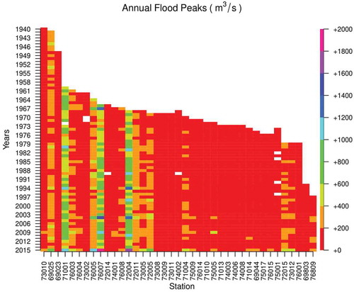
An AM series of river flow data was obtained from the National River Flow Archive for a total of 39 catchments located in the northwest of England (NRFA 2018). The last water year available in the AM series data was 2015. The characteristics of the investigated river stations are shown in Table A1 in the Appendix, as well as in Fig. 1. Additionally, regional climate datasets for northwest England were obtained from the UK’s national weather service, the Met Office. Specifically, monthly rainfall (mm) and temperature (°C) for the years from 1910 to 2018 were obtained and matched to the river flow recording periods.

Figure 1. Annual maximum series of flood flows observed between 1940 and 2015 in the study region (station ID numbers are indicated on the x axis; records are arranged from longest to shortest)

2.2 Non-parametric tests

A preliminary analysis of the AM series was performed to detect changes in the frequency regime. In particular, two well-known and widely used non-parametric tests, in which no explicit assumption about the parent distribution for the data is made, were utilized in this study to detect any significant change in the annual maximal flood peak series, namely the non-parametric Mann-Kendall test (MKT) and the Pettitt test (PT) (see Kendall 1975, Pettitt 1979, Douglas et al. 2000). MKT is widely used to identify significant monotonic upward or downward trends in hydro-meteorological data series, while PT is used to detect sudden changes in the mean (and/or the variance) of the time series.

2.3 Frequency distribution model

The GLO distribution model is the recommended distribution curve for flood frequency analysis in the UK (Reed and Robson 1999). For this reason, it is employed here instead of the more commonly used GEV distribution. In this regard, the cumulative distribution function of the GLO distribution, F(x), is shown as follows (Hosking and Wallis 2005):

(1) $F\left(x\right)=\frac{1}{1+e^{-y}}y=\left\{\begin{array}{c}-{\xi }^{-1}\times log\left(1-\xi \times \frac{x-\mu }{\sigma }\right)\xi \ne 0\\ \frac{x-\mu }{\sigma }\xi =0\end{array}\right.$(1)

The corresponding GLO quantile function, the inverse of F(x), corresponding to a given recurrence interval, x(F), is given by Equation (2)(2) $x\left(F\right)=\left\{\begin{array}{c}\xi +\sigma \frac{\left[1-{\left\{\frac{1-F}{F}\right\}}^k\right]}{K}\xi \ne 0\\ \xi -\sigma log\left\{\left(1-F\right)F\right\},\xi =0\end{array}\right.$(2) , where F is the cumulative function shown in Equation (1)(1) $F\left(x\right)=\frac{1}{1+e^{-y}}y=\left\{\begin{array}{c}-{\xi }^{-1}\times log\left(1-\xi \times \frac{x-\mu }{\sigma }\right)\xi \ne 0\\ \frac{x-\mu }{\sigma }\xi =0\end{array}\right.$(1) (Hosking and Wallis 2005):

(2) $x\left(F\right)=\left\{\begin{array}{c}\xi +\sigma \frac{\left[1-{\left\{\frac{1-F}{F}\right\}}^k\right]}{K}\xi \ne 0\\ \xi -\sigma log\left\{\left(1-F\right)F\right\},\xi =0\end{array}\right.$(2)

The location, scale and shape parameters are denoted μ, σ and ξ, respectively.

2.4 Parametric non-stationary framework

Whereas in the classical stationary setting, all parameters are constant (Model 1), in the non-stationary framework the statistical properties of distributions can be specified as a function of different predictors. Six non-stationary models (Models 2–7) are introduced in this study, allowing the location parameter to change linearly as a function of the predictors. The scale and shape parameters are considered constant in all models. The reason the shape parameter is treated as constant is the fact that reliably achieving its correct value is generally challenging (Salas and Obeysekera 2014). In addition, preliminary analyses performed for the study area clearly indicated the hypothesis of a time-varying scale parameter is not statistically significant for the vast majority of stations, therefore we assumed the scale parameter to be constant in our study.

The first explanatory variable integrated into the parameter was time – that is, the years over which the flood happened (Model 2). Time can be viewed as a proxy for the identification of time-varying physical drivers, which are causing the change in the annual flood series (e.g. land-use and land-cover dynamics). As a further step, physically based covariates were included to help identify the flood changes and, therefore, to yield a better fit over the data. Hence, annual precipitation was included in the next step (Model 3). Although extreme precipitation is often used as covariate in the literature (Villarini et al. 2009b, Prosdocimi et al. 2014), annual rainfall is considered in this study. This is because Salas and Obeysekera (2014) determined that annual rainfall as a predictor can represent non-stationary behaviour more accurately than short-term extreme precipitation events can. This is because annual precipitation and event extreme precipitation are usually correlated, and annual precipitation has long-term impacts on the development of catchment characteristics (Salas and Obeysekera 2014). The other reason is that annual precipitation influences the antecedent soil moisture of each single event, ultimately influencing flood magnitudes (Gaál et al. 2012). Further, annual temperature was included as a covariate (Model 4) as a proxy for evapotranspiration. To provide additional alternatives, which may help produce a more accurate fit, Models 5, 6 and 7 were constructed as additive models combining the aforementioned covariates. In summary, the following models are employed:

• → Model 1, stationary model in which all parameters are constant, $\mu ,\sigma ,\xi$

• → Model 2, non-stationary model in which location parameter varies linearly with time (t), $\mu \left(t\right)=B_{2,0}+B_{2,1}\times t,\sigma ,\xi$

• → Model 3, non-stationary model in which location parameter varies linearly with annual rainfall (R), $\mu \left(R\right)=B_{3,0}+B_{3,1}\times R,\sigma ,\xi$

• → Model 4, non-stationary model in which location parameter varies linearly with annual temperature (T), $\mu \left(T\right)=B_{4,0}+B_{4,1}\times T,\sigma ,\xi$

• → Model 5, non-stationary model in which location parameter varies linearly with both time (t) and annual rainfall (R), $\mu \left(t,R\right)=B_{5,0}+B_{5,1}\times t+B_{5,2}\times R,\sigma ,\xi$

• → Model 6, non-stationary model in which location parameter varies linearly with both time (t) and annual temperature(T), $\mu \left(t,T\right)=B_{6,0}+B_{6,1}\times t+B_{6,2}\times T,\sigma ,\xi$

• → Model 7, non-stationary model in which location parameter varies linearly with both annual rainfall (R) and annual temperature (T), $\mu \left(R,T\right)=B_{7,0}+B_{7,1}\times$ $R+B_{7,2}\times T,\sigma ,\xi$

where μ is the location parameter, σ is the scale parameter, ξ is the shape parameter and t is the water year associated with each AM event. Note that time (t) is considered from the first observation record for each river gauge station until the end of the flow observations (water year 2015). R and T represent cumulative annual rainfall depth and annual temperature, respectively, for northwest England ending in water year 2015. $B_{m,i}$ with m (model) varying from 2 to 7 and i = 0,1,2 are unknown regression coefficients which need to be estimated based on the available annual maximum series, in order for the location parameter to be calculated.

2.5 Parametric estimation

The unknown parameters of seven GLO distribution models defined in section 2.4 are estimated using the MLE method (Coles et al. 2001, Katz 2013). If $X=\{X_1,X_{2,....}{X}_n\}$ are observations from the distributed random variables, coming from a probability distribution model f with parameters P, the MLE measure maximizes the likelihood function, given by:

(3) $L\left(\mathit{P}\right)=\prod _{i=1}^{n}f\left(X_i;\mathit{P}\right)$(3)

However, it is often easier to work with the log-likelihood, instead of the likelihood function, given by Equation (4)(4) $L\left(\mathit{P}\right)=log\left[L\left(\mathit{P}\right)\right]=\sum _{i=1}^{n}log\left[f\left[X_i;\mathit{P}\right]\right]$(4) :

(4) $L\left(\mathit{P}\right)=log\left[L\left(\mathit{P}\right)\right]=\sum _{i=1}^{n}log\left[f\left[X_i;\mathit{P}\right]\right]$(4)

The log-likelihood function for the GLO distribution function is then shown below:

(5) $\mathrm{l}\mathrm{o}\mathrm{g}\left(F\left(x\right)\right)=-log\sigma +\left(\frac{1}{k}-1\right)\times \mathrm{\Sigma }log\left(1-\left(\frac{X-\mu }{\sigma }\right)\times \xi \right)-2\times \sum log(1+(1-{\left(\frac{X-\mu }{\sigma }\right)}^{\frac{1}{k}}$(5)

Thus, the MLE finds the values of the parameters of the log-likelihood that make the observed data sample most likely and, finally, delivers the estimated parameters. In this study, non-linear optimization using the maxLik package (Henningsen and Toomet 2011) was carried out in R software (R Development Core Team 2013), utilizing the Newton-Raphson algorithm, for numerically optimizing the log-likelihood function of the GLO models.

2.6 Selection of the best model

The Akaike information criterion (AIC, Akaike 1974) is a goodness-of-fit measure that aids in comparing frequency models and selecting the best-fitting one. It represents how well the model fits over the data relative to the other frequency models. The AIC equation is as follows:

(6) $AIC=\left[2k-2log\left(L\right)\right]$(6)

in which L is the maximum value of the log-likelihood function, and k is the number of parameters. The smaller the AIC value, the better the model performs, in comparison to other models. This implies that the best model is recognized based on the balance between the goodness of fit (i.e. the value of the log-likelihood) and the model complexity (i.e. the number of parameters).

Additionally, confidence intervals for the regression parameters for each predictor were derived using the delta method (Salas and Obeysekera 2014): these were used to check whether the inclusion of a predictor into the model is significant at the 5% significance level. The literature presents various approaches to construct confidence intervals, such as the delta method, bootstrap method, and profile likelihood method (Efron and Tibshirani 1994, Royall 1997). Although profile likelihood might deliver a more robust and accurate estimation of the uncertainties (due to assuming the asymmetrical characteristics of maximum likelihood estimates), it is oftentimes computationally demanding and burdensome (Obeysekera and Salas 2014). In contrast, using locally computed derivatives (e.g. the delta method) can be relatively accurate but computationally easy and more efficient. This justifies the popularity of the delta method as an approach to assess uncertainties in the parameters and their transformations (e.g. quantiles) in the literature (see e.g. Macdonald et al. 2014, Obeysekera and Salas 2014, Šraj et al. 2016). This method is also used herein to calculate the uncertainties for the quantile estimations at the 95% confidence level.

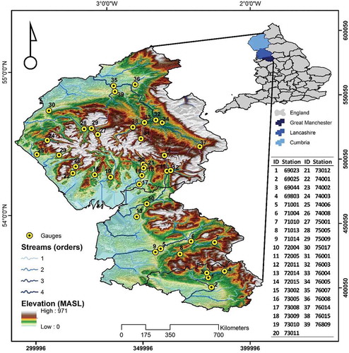
2.7 Study area

A total of 39 AM series of peak flow obtained from river gauging stations located in the northwest of England (Cumbria, Lancashire and the Greater Manchester area) are considered in this study (Fig. 2). These stations were chosen due to their locations on rivers that have recently experienced extraordinary flood events, in 2004, 2009 and 2015. The study area as well as the locations of the river stations are illustrated in Fig. 2. During storm Desmond, 4–6 December 2015, almost all of the gauges investigated in Cumbria observed discharges that exceeded their previous records. This region of England is targeted in this study because of the exceptional nature of the inundation events that have occurred there over the past few years (Miller et al. 2013). Topological ordering of the rivers over the investigated catchments is represented as well, in terms of Strahler stream order (Strahler 1957) as shown in Fig. 2.

Figure 2. Study area and the location of river gauging stations considered in the study

3 Results and discussion

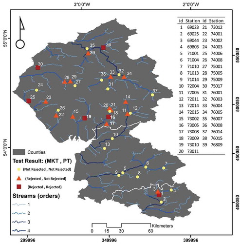
First, AM series for all 39 stations were tested for trends and sudden changes, or change-points, via the MKT and PT, respectively. Figure 3 shows the spatial pattern of MKT and PT results. The MKT detected the presence of statistically significant trends (at the 5% significance level) at 20 stations. Note that all monotonic trends detected across the study region are upward. The majority of series characterized by statistically significant trends are scattered around the Northern region of the study area (e.g. Cumbria). Additionally, PT detected significant sudden changes in the mean of the time series at six stations across the study area. Note that the same six stations for which PT detected statistically significant sudden changes are also flagged by MKT as series characterized by statistically significant upward trends. That is, both tests detect significant changes in these series, which could be interpreted as trends or abrupt changes.

Figure 3. Mann-Kendall test (MKT) and Pettitt test (PT) results in terms of rejection of the null hypothesis (i.e. MKT: presence of a monotonic trend; PT: presence of an abrupt change in the mean) for the study sequences of annual floods (at the 5% significance level)

Second, based on the results of the non-parametric tests, the seven stationary and non-stationary distribution models introduced in section 2.4 were estimated using peak flow series from each of the 39 stations in turn. Although the implications are depicted for all of the 39 stations in the form of spatial maps (described and shown in the following sections), only results for stations number 69044 (located in Greater Manchester) and 75005 (located in Cumbria and Lancashire) with at least 40 years of observations are presented here in more detail to showcase the outcome of the study; detailed results for all stations can be found in the Supplementary material.

3.1 Identification of the best-fit models

3.1.1 Station no. 69044: River Irwell at Bury Ground

Results from fitting the model parameters by the MLE method, along with the ranking based on the AIC, are presented in detail in Table 1 for River Irwell at Bury Ground. The results show that Model 2, where time is included as the only covariate, is not statistically different from zero, as B_2,1 encompasses zero. However, when annual rainfall is included as an additional step (Model 3), the corresponding estimated parameter, B_3,1, is found to be significantly different from zero at the 5% significance level (i.e. the 95% confidence interval does not contain zero). This indicates that the inclusion of annual rainfall is able to explain a large part of the variability of the peak flow series.

Table 1. Parameters of stationary and non-stationary models estimated by the MLE method for station no. 69044: River Irwell at Bury Ground

Station no. 69044: River Irwell at Bury Ground
Parameters	μ			σ	ξ	AIC	Rank
	B0	B1	B2
Model 1:S	105.851 [95.18; 116.52]	-	-	19.374	−0.206	412.05	5
Model 2: μ(t)	95.584 [77.25; 113.92]	0.502 [−0.26; 1.26]	-	19.020	−0.204	412.37	6
Model 3: μ(R)	−12.225 [−91.13; 66.68]	33.662 [11.15; 56.18]	-	17.477	−0.195	405.57	1
Model 4 μ(T)	10.867 [−124.3; 146.03]	10.765 [−4.581; 26.11]	-	18.956	−0.190	412.03	4
Model 5: μ(R, t)	−10.873 [−88.27; 66.52]	31.192 [8.71; 53.67]	0.330 [−0.34; 1]	17.409	−0.223	406.72	2
Model 6: μ(t, T)	32.152 [−114.41; 178.71]	7.661 [−9.91; 25.23]	0.298 [−0.59; 1.19]	18.876	−0.194	413.6	7
Model 7: μ(R, T)	−49.163 [−179.68; 81.35]	31.340 [8.09; 54.59]	5.105 [−8.96; 19.17]	17.421	−0.190	407.05	3

When incorporating temperature as a covariate (Model 4), its parameter, B_4,1, was not found to be significantly different from zero. In particular, the estimated confidence intervals for the parameters of all time- and temperature-dependent regression models (Models 2, 4 and 6) – that is, B_2,1, B_4,1, B_6,1 and B_6,2 – do in fact contain zero. Despite the improvement over the stationary fit when both rainfall and time (Model 5) and rainfall and temperature (Model 7) are included, the AIC measure indicates that including only annual rainfall as a covariate yields the best-fitting model. This implies that allowing the location parameter of the GLO frequency model to vary as a linear function of annual rainfall (as the only covariate) expressed the alterations in flood peaks more accurately than the other covariates and, thus, gave a better fit of the data.

3.1.2 Station no. 75005: River Derwent at Portinscale

The second station explored in detail is station no. 75005. Table 2 shows the estimated parameters (along with the limits of the 95% confidence intervals) and ranking of all models by the MLE and AIC. According to the table, the inclusion of time and temperature (Models 2 and 4) did not produce a statistically significant change in the model fit. On the other hand, the inclusion of annual rainfall in all models (Models 3, 5 and 7) into the location parameter – B_3,1, B_5,1 and B_7,1, respectively – significantly improved the stationary model’s fit. This is supported by AIC ranking alongside the confidence limit around the B₁ parameter, which indeed does not encompass zero.

Table 2. Parameters of stationary and non-stationary models estimated by the MLE method for station no. 75005: River Derwent at Portinscale

Parameters	Station no. 75005: River Derwent at Portinscale
	μ			σ	ξ	AIC	Rank
	B0	B1	B2
Model 1: S	102.926 [93.19; 112.66]	-	-	19.327	−0.338	445.38	6
Model 2: μ(t)	91.398 [76.67; 106.13]	0.526 [−0.01; 1.06]	-	18.496	−0.344	443.62	4
Model 3: μ(R)	10.106 [−44.11; 64.32]	26.1 [10.85; 41.35]	-	16.630	−0.376	435.61	1
Model 4: μ(T)	88.057 [−25.67; 201.78]	1.686 [−11.17; 14.5]	-	19.291	−0.334	447.32	7
Model 5: μ(R, t)	14.705 [−41.46; 69.61]	24.11 [7.37; 40.85]	0.145 [−0.4; 0.69]	16.524	−0.368	437.34	3
Model 6: μ(T, t)	141.367 [38.91; 243.83]	−6.019 [−18.24; 6.2]	0.667 [0.06; 1.28]	18.366	−0.359	444.76	5
Model 7: μ(R, T)	37.487 [−34.62; 109.59]	28.508 [12.32; 44.7]	−4.074 [−12.2; 4.04]	16.556	−0.397	436.8	2

However, according to the AIC goodness-of-fit measure, Model 3, with only annual rainfall as covariate, was found to be the best model to explain the ongoing changes in the peak river flow regimes, compared to the other models. A detailed examination of the flood peaks and annual precipitation for this streamgauge also demonstrates that the maximum annual rainfall (119 mm) observed in northwest England in 2015 is associated with the second highest river flow (365 m³/s), which happened in the same year, the main reason for which could be the intense precipitation that occurred in November and December 2015. This measure is, again, highlighting the relevance of annual rainfall as covariate to help ascertain the changes in flood frequency.

3.1.3 Identification of the best-fit models at all streamgauges

Both stationary and non-stationary frequency analyses using the GLO distribution were repeated at all 39 gauging stations in the study area; the detailed results can be found in the Supplementary material (Tables S1–S39). The selected frequency models at all stations, as decided by the AIC measure, are shown in Fig. 4. This highlights that the stationary Model 1 was preferred at only three streamgauges out of 39, meaning that treating the location parameter as a constant value at these stations revealed a better performance and fit to the data, as opposed to 36 stations at which non-stationary settings were found to give a better fit to the data. This indicates that the driving factors such as meteorological conditions and time largely influenced the flood characteristics in northwest England. Non-stationarity, thus, might be a dominant process at most gauges, urging authorities and designers to take non-stationarity into account as an option for the future construction of flood defence structures alongside conventional methods. Moreover, annual rainfall rather than time and temperature is often included in the best-fit models, indicating that this variable explains a large proportion of the variability in the peak flow samples. At 22 stations out of 39, the regression model with only annual rainfall as the explanatory variable (Model 3) was preferred, as the best fit. These findings are in agreement with the other studies in the literature (Prosdocimi et al. 2014, Šraj et al. 2016), which reported improvement over stationary performance when rainfall is included in the frequency analysis in preference to the time-based models.

Figure 4. Best-fit distribution model in northwest England, based on the Akaike information criterion (AIC) measure

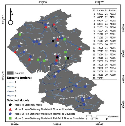
According to Fig. 4, eight and six stations where the regression models were fitted with time (Model 2) and with rainfall and time (Model 5), respectively, were found to maximize the AIC measure, making a significant improvement over the stationary fit. Note also that all the regression models incorporating temperature as a covariate (Models 4, 6 and 7) underperformed relative to other options at all streamgauges. This indicates that temperature appeared to be a poor predictor for change in the peak flow values. In other words, temperature (as a proxy for evapotranspiration) is not a good descriptor of the frequency of the flooding process and, hence, was not able to accurately detect the changes in the flood characteristics in the study area. It is worth highlighting that Model 3, where annual rainfall was integrated as the only covariate, was preferred at all streamgauges in the south of the study area (i.e. Greater Manchester and Lancashire), whereas Cumbria, located in the north, reported more diverse preferred models (i.e. Models 1, 2, 3 and 5).

It is worth noting that MKT did not detect statistically significant changes at three stations for which the stationary framework provided the best fit. Also, at 16 gauges with statistically non-significant trends, non-stationary models (mostly precipitation-included models) outperformed the stationary one (Figs 3 and Figs 4). Bertola et al. (2019) reported similar results; they show superior performance for rainfall-driven non-stationary models even at gauging stations without statistically significant trends.

3.2 Resorting to non-stationary models for quantile estimation

Flood return period is a key concept for the design of hydraulic facilities and flood control systems. For “stationary” models with constant parameters, the probability p that a flood peak will be larger than a certain design event Q_T in a year is expressed in terms of the return period T, which is the inverse of p (i.e. T = 1/p). On average, a T-year flood is exceeded once in T years. Therefore, a 100-year flood event has a probability of 1% of occurring or being exceeded in 1 year. These simple relationships between design events, exceedance probability and return period rely on the assumptions that the probability distribution of high flows is constant in time: this is not the case for the non-stationary models.

There is a large body of literature on the need to revise the concept of the return period and on the possible adaptation of this quantity in the context of non-stationary conditions (Cooley 2013, Obeysekera and Salas 2014, Salas and Obeysekera 2014, Volpi 2019). In particular, there are two main approaches to flood return period approximation under non-stationary conditions: (a) using the concept of expected waiting time for the first occurrence of a flood event exceeding the design flood (Salas and Obeysekera 2014), and (b) defining the return period as the time interval in years for which the expected number of exceeding flood events is equal to 1 (Cooley 2013).

Instead of resorting to either of the revised definitions listed above, we decided to discuss the practical implications of adopting the non-stationary models presented above to estimate the flood quantiles at a given location, by calculating the at-site flood quantiles for any given year by using the distribution parameters as estimated for that year (e.g. referring to the cumulative rainfall depth of that year). Once the parameters of the seven models (one stationary and six non-stationary) are estimated and the best-fit model is identified based on the AIC criterion, the flood quantiles for specific recurrence intervals and different models can be quantified and compared. This will allow for a direct assessment of the impact of non-stationary frequency models, for example on design events.

Sections 3.2.1 and 3.2.2 present and compare the estimates for a rare and median flood (i.e. a one-in-T-years, or T-year flood, with T being conveniently large; and a 2-year flood) at the two aforementioned test site stations (see Figs 5 and Figs 6). According to report no. 629 from the Flood Defence Standards for Designated Sites (Risk & Policy 2006), the 100-year flood event is generally considered for constructing flood defences in most parts of the UK, and for this reason we selected T = 100 years in our study. Section 3.2.3 focuses on the 100-year flood and addresses the implications and potential consequences of selecting a stationary or a non-stationary model at all streamgauges when designing flood defences and flood risk mitigation measures.

Figure 5. Comparison of the estimated 2-year (median) and 100-year (design) flood quantiles for stationary and best-fit non-stationary model at gauging station Rock (69044)

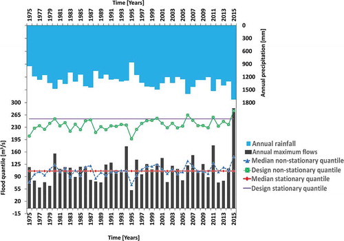
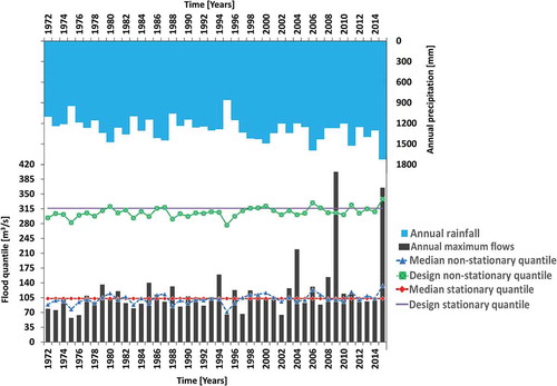
Figure 6. Comparison of the estimated 2-year (median) and 100-year (design) flood quantiles for the stationary and best-fit non-stationary model at gauging station Derwent (75005)

It should be pointed out that it is not quite straightforward to answer which (design) discharge should be taken into account for flood risk management when they are associated with non-stationary outcomes (Serinaldi and Kilsby 2015). This is due to the changing characteristics of non-stationary frequency analysis over time. As a result, we take the last year of the fitting period (2015), as advised by Luke et al. (2017), to select and compare the (design) quantiles between non-stationary and stationary estimates throughout this study. However, to better showcase and represent the practical implications of our study, results for the second-to-last year (i.e. 2014) are included as well, and compared with those for 2015.

3.2.1 Comparison of the 2- and 100-year flood quantiles at Station no. 69044: River Irwell at Bury Ground

Considering Irwell at Bury Ground, as shown in Fig. 5, where only the stationary and best-fit non-stationary estimates are displayed, incorporating annual rainfall as a covariate in the location parameter led to an abrupt change for both median and design flood estimates moving from one year to the next, as opposed to the stationary model for which the flood quantile is constant. Differences between stationary and the best-fit non-stationary model predictions become more apparent at larger return periods in the flood estimations. This is attributed to the occurrence of larger uncertainties for non-stationary settings at higher frequencies. The stationary model predicted the median to be 105.85 m³/s, as opposed to the best-fit non-stationary model (driven by cumulative annual rainfall), which predicted a median of 146.79 m³/s in the last year of the fitting period. This value is approximately 40% greater than the value predicted by the classic stationary setting.

This river also shows an abrupt increase in the median flood flows in the late 1990s, alongside three sharp spikes in 2007, 2011 and 2015 (Fig. 5). Given the strong correlation between annual precipitation totals and annual floods for this catchment, these spikes are a consequence of the considerable amount of cumulative annual precipitation that occurred in these years (above 1500 mm in all three cases). For instance, the highest annual precipitation (1724 mm) is associated with the largest observed discharge (284 m³/s), which occurred in 2015.

In terms of the 100-year flood (i.e. the design flood quantile; see Fig. 5), similar to the median (i.e. the 2-year flood), the best-fit non-stationary model was able to capture the design floods based on precipitation values occurring in each year. For example, the non-stationary model predicts the largest design flood (i.e. 276.85 m³/s) in 2015, reflecting the highest value observed for the cumulative annual precipitation value, that occurred in the same year. Furthermore, the design flood (100-year flood) estimated under the best-fit non-stationary condition (Model 3) is associated with the 160-year quantile under stationary conditions. This implies that there might be a 60-year frequency difference between the stationary (254.2 m³/s) and non-stationary (276.85 m³/s) setting in the last year of the flood records.

Nonetheless, since the 95% confidence limit becomes wider for the non-stationary estimate resulting from Model 3 (see Table A2 in the Appendix) compared to the stationary one, the interpretation of change in the design quantile is not straightforward. As shown in Table A2, inspecting the confidence interval around the stationary and the preferred non-stationary quantile does not allow us to infer whether we have certainly (at least with 95% confidence) underestimated the design quantile using the stationary setting. These findings emphasize the importance of incorporating uncertainty analysis in non-stationary flood risk management schemes.

3.2.2 Comparison of the 2- and 100-year flood quantiles at station no. 75005: River Derwent at Portinscale

Comparing median and design flood quantiles for River Derwent at Portinscale (Fig. 6), the same interpretations as above can be made. As stated in section 3.2.1, the non-stationary model, where cumulative annual rainfall was integrated, generated jumps. The median and design quantile exhibit a similar pattern over the flood period, with larger differences between the flow estimates of the 100-year events. The median quantiles estimated by the regression model are consistently larger than the one obtained by the stationary model in the late 1990s, especially after 2006.

Moreover, the 100-year quantile of the rainfall-dependent model (Model 3), with 338.36 m³/s discharge in the last year, can be associated with the 140-year flood quantile of the stationary model. It stands to reason that the rate of increase in the non-stationary design quantile might have been 7%. However, the implication of change between design quantiles based on the stationary and the preferred non-stationary model is complicated, as their 95% confidence intervals overlap (see Table A2).

3.2.3 Practical implications of selecting non-stationary vs stationary design quantiles

To assess the implications of selecting a non-stationary vs a stationary model for estimating the design flood quantile (as a measure of constructing flood defences in most parts of the UK) in northwest England, the approach outlined above was repeated at all 39 stations with a specific focus on the 100-year return period.

In this context, to investigate the discrepancy between the design values, we measure the ratio between the design quantiles derived from the preferred non-stationary model (in case a non-stationary model was selected by the AIC criterion) in 2015 (the last year for which data is available), and the stationary one at each river station (Fig. 7(a)). Furthermore, uncertainties around the design quantiles are shown in Table A2 of the Appendix for all stations (represented by confidence limits). To further showcase and support the implications of our framework, the same procedure performed and explained above was repeated for the second-to-last year in our sample (i.e. 2014), shown in Fig. 7(b). The importance of evaluating different windows of records was also emphasized by Griffin et al. (2019).

Figure 7. Ratio of the best-fit non-stationary design flood quantile to the stationary one in northwest England in (a) 2015 and (b) 2014. For the stations highlighted in red, the stationary model and the best-fit non-stationary model produce significantly different flood quantile predictions at the 95% confidence level (top right tables list gauging stations and their ID numbers)

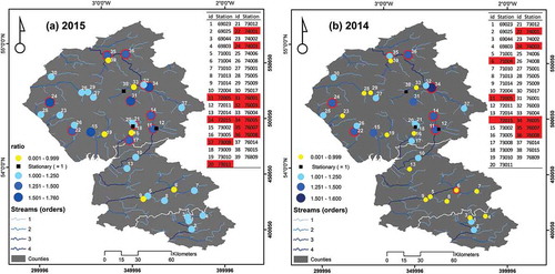
According to the results shown in Fig. 7(a), the stationary distribution produced the best fit at three stations (black squares). At six stations (shown in yellow), non-stationary analysis reduced the stationary estimates in 2015. At all of the remaining stations, in contrast, the non-stationary regression models might have increased over the conventional stationary design estimate. The most significant increase is observed mainly in the north of the study area (Cumbria). This finding, however, alongside the design events’ confidence limits (see Table A2) makes it difficult to conclude whether the stationary models do effectively underestimate or overestimate the quantile when compared to the non-stationary ones in 2015. For instance, the flow estimate resulting from the best-fit non-stationary model at gauge 73002 was around 75% higher (the largest change across the area) than the one predicted by stationary model. However, by looking at their associated uncertainties (Table A2), it is not possible to properly judge the estimation of quantiles. This is because the confidence interval associated with the non-stationary model becomes wider compared to the stationary one, and indeed, they overlap with each other.

However, based on the achieved uncertainties shown in Table A2, we can infer with 95% confidence that at only 11 stations out of 39, stationary models underestimated the quantiles compared to non-stationary ones in 2015. These gauges (highlighted in red in Fig. 7(a)), all located in Cumbria, are the ones that were severely hit with floods, especially in that year, producing tremendous discharge rates up to 65% higher than the stationary estimates. This conveys a crucial message, that the non-stationary framework for designing hydraulic facilities in northwest England should be considered as an alternative option along with the traditional stationary setting, with special attention to such stations with severe flood records.

Comparing the results (see Table A2 and the Supplementary material), for example at station no. 72005 on River Lune at Killington, with those of a similar study (Faulkner et al. 2020) demonstrates a notable difference in terms of the design flood event in water year 2015. The stationary and the best-fit non-stationary design event in the earlier study was calculated at around 575 m³/s [450; 700] and 600 m³/s [550; 750], respectively. However, the same quantities were calculated as 622.08 m³/s [583.51; 665.98] and 878.63 m³/s [820.24; 937.02] in the present study. This implies a 4% and 46% discrepancy with respect to the stationary and non-stationary design flood event, respectively, at this gauge. This is attributed to the selection of a different frequency distribution (i.e. GEV distribution) by Faulkner et al. (2020). Although the inclusion of time was found to be significant both by Faulkner et al. (2020) and in this study, the simultaneous incorporation of rain and time here gave the preferred fit at the investigated station – which can be viewed as the part missing from the literature.

In addition to the implications for the last year in the record (2015), in which the highest ever total rainfall accumulation was recorded, Fig. 7(b) illustrates the ratios of the best-fit non-stationary design quantiles to the stationary ones for 2014 (the second-to-last year in the dataset). This figure shows patterns of the ratio that are very similar to those depicted in Fig. 7(a) (particularly in Cumbria). Also, the gauges highlighted in red (i.e. those where stationary distribution underpredicts flood quantiles at the 95% confidence level) show close similarity for both years, even though 2014 was not an extremely wet year (1302 mm cumulative annual rainfall) relative to 2015 (1724 mm cumulative annual rainfall).

3.3 Non-stationary design flood quantiles

To provide insight regarding how the design event might have changed between the stationary and the best-fit non-stationary analysis in the last year of observations, Fig. 8a shows the results produced by dividing the non-stationary design quantile by the stationary one in 2015, and accordingly obtaining the design “trend.” Similar to the previous section, results obtained by referring to 2015 have been compared with those associated with 2014 (Fig. 8b) to better draw the practical implications for the design quantiles.

Figure 8. “Trend” map of the design flood quantiles in northwest England in (a) 2015 and (b) 2014, representing how design quantile estimates differ from the stationary estimates (top right tables list gauging stations and their ID numbers)

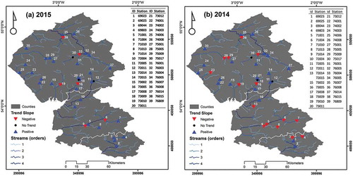
As shown in Fig. 8a, the vast majority of stations (30 stations) recorded larger non-stationary design values with respect to the stationary ones – that is, an upward “trend” – supporting the conclusion that it is likely that large flood events might happen again in the future in those areas. In contrast, six stations revealed downward behaviour, which means that the preferred non-stationary models accounted for lower quantiles compared to the stationary ones. However, the implementation of uncertainties (e.g. confidence intervals as in Table A2) for both stationary and non-stationary analysis should be an integral part of any conclusion, all of which helps in detecting the ongoing changes in the flood peak magnitudes.

When it comes to the comparison of quantiles’ sensitivity to the selected predictors between 2014 and 2015 (Fig. 8(a) and (b)), we observe an analogous situation across the region, as discussed. In other words, most river stations – especially in the North – show exactly the same setting in 2014 and 2015. The situation is slightly different in the south (Lancashire), where there is a positive signal (increasing estimates, blue triangle) for 2015 but a negative signal (downward estimates, red triangles) in 2014.

This indicates that flood hazard can be quite sensitive (especially in the south) to the changes in annual rainfall totals in the study region, and previous studies clearly pointed out significant changes in observed mean annual precipitation across the study area between 1960 and 2000 (i.e. mean annual precipitation between 1960–1990 and between 1970–2000), showing increases as high as 15% in Cumbria (Jenkins et al. 2007).

It is worth mentioning that common methods to quantify risk are based on the assumption that the distribution of the phenomenon under study (e.g. flooding) is unchanged. Although alternative methods to quantify risk under changing conditions have been proposed (Parey et al. 2007, 2010, Villarini et al. 2009a, Rootzén and Katz 2013, Salas and Obeysekera 2014), there is still no standard paradigm to assess risk when using models that allow for change. When it comes to time-dependent models, extrapolation of the future design quantiles can be unrealistic, as the change happening in the future might not happen the same way as it did in the past. Utilizing physically based predictors, on the other hand, establishes a relationship between covariate and variable (flood flows), yielding a better fit – however, potential future risk assessment would depend on the unknown future distribution of the physical covariate. Further, the relationship between the variable of interest and the physical covariate would need to remain the same. Given these methodological challenges, we do not attempt to assess future flood risk in northwest England but simply present the implications of the present-day (i.e. year 2015) conditions relative to the second-to-last year in our sample (i.e. 2014).

4 Summary and conclusions

This study investigated the presence of non-stationarity in annual maxima (AM) of river peak flow data series for numerous catchments across northwest England. The study was motivated by the concerns over the suitability of traditional procedures for the estimation of flood frequencies following the successive extreme floods in 2004, 2009 and 2015 in northwest England. Taking into account the indirect impact of climate/human-induced attributes, a linear regression model for the location parameter of the generalized logistic (GLO) frequency distribution model was constructed, where explanatory variables such as time, annual rainfall, and annual temperature, alongside their linear combinations, were integrated. In this context, maximum likelihood estimation (MLE) and the Akaike information criterion (AIC) were applied to the frequency models at 39 river gauging stations across the northwest of England to infer the estimated parameters and choose the best-fitting model, respectively. Our analysis revealed that 36 river stations demonstrated non-stationary behaviour, implying that the flood characteristics are changing over time. However, three gauges recorded no significant changes in any of their models’ parameters (i.e. stationary behaviour was dominant). Among non-stationary-dominated streamgauges, the best model often included annual rainfall as the predictor, signifying that annual rainfall is the climatic driver most responsible for changes in the flood characteristics in northwest England.

Moreover, a general implication of this study for flood quantiles is that most rivers in the area showed a sharp increase in higher quantiles in the late 1990s, with an even sharper increase within the last 10 years of the recording period. This implies that the stochastic process of the distribution underlying peak flows might be changing in most cases, especially in recent years; the impact of this should be incorporated into the design of future hydraulic facilities. Hence, we highly recommend the consideration of a non-stationary framework alongside the traditional stationary analysis in northwest England, especially in the Cumbria region, as these implications can be put into practice (in the light of uncertainty analysis) and, finally, help in predicting the ongoing alterations in the flood frequency. This would prompt local flood managers to enhance the current flood management plans and reduce the flood risk.

Despite the notable improvements over the stationary fit, resulting from the physically based non-stationary distributions (e.g. when rainfall is included as covariate), further research needs to be carried out towards the estimation of the frequency distribution for the covariate itself. This means that when introducing an extra stochastic component such as annual rainfall into the model, there should be an additional study on whether the stochastic component is stationary or not. Future studies could also potentially consider different precipitation indices as covariates in a non-stationary framework, such as design rainfall quantiles or seasonal rainfall characteristics, selecting those that are more aligned with the seasonality of floods and processes driving the flood production mechanism in the study area.

Acknowledgements

The authors gratefully acknowledge the UK National River Flow Archive (NRFA) and National Weather Service (Met Office) for providing the river flow and climate data, respectively.

Disclosure statement

No potential conflict of interest was reported by the authors.

Supplementary material

Supplemental data for this article can be accessed here.

Appendix

Table A1. Characteristics of all 39 river gauging stations in the study area. AOD: above ordinance datum

Station number	Station level (m AOD)	River name	Location	Catchment area (km^2)	Period of record	Sample records (years)	Maximum flow (m^3/s)
69023	62.9	Roch	Blackford Bridge	186	1948–2015	68	192
69025	24.2	Irwell	Manchester Racecourse	557	1941–2015	75	700
69044	79.8	Irwell	Bury Ground	139.9	1975–2015	41	284
69803	N/A	Roch	Rochdale	111	1993–2015	23	92.8
71001	9.5	Ribble	Samlesbury	1145	1960–2015	55	1100
71004	39.9	Calder	Whalley Weir	316	1970–2015	46	501
71010	92.3	Pendle Water	Barden Lane	108	1972–2015	44	197
71013	98.3	Darwen	Ewood	39.5	1973–2015	43	60.3
71014	8.1	Darwen	Blue Bridge	128	1974–2015	42	218
72004	10.7	Lune	Caton	983	1968–2015	48	1740
72005	82.8	Lune	Killington	219	1969–2015	47	627
72011	84.1	Rawthey	Brigflatts	200	1968–2015	48	460.4
72014	16.6	Conder	Galgate	28.5	1966–2015	49	33.7
72015	165	Lune	Lunes Bridge	141.5	1979–2015	37	409
73002	38.6	Crake	Low Nibthwaite	73	1962–2015	52	51
73005	18.9	Kent	Sedgwick	209	1968–2015	48	527
73008	10.9	Bela	Beetham	131	1969–2015	47	129
73009	34.6	Sprint	Sprint Mill	57.5	1969–2015	47	94.8
73010	37.3	Leven	Newby Bridge	247	1940–2015	76	224
73011	50.3	Mint	Mint Bridge	65.8	1969–2015	47	170
73012	N	Kent	Victoria Bridge	183	1979–2015	37	403
74001	14.8	Duddon	Duddon Hall	85.7	1967–2015	49	267.9
74002	54.2	Irt	Galeyske	44.2	1968–2015	47	35.9
74003	110.4	Ehen	Bleach Green	44.2	1973–2015	43	102.44
74006	26.4	Calder	Calder Hall	44.8	1973–2015	43	173.17
74008	75.9	Duddon	Ulpha	47.9	1973–2015	43	103.71
75001	159.5	StJohns Beck	Thirlmere Reservoir	42.1	1974–2015	38	75.4
75005	72.6	Derwent	Portinscale	235	1972–2015	44	402.36
75009	99.7	Greta	Low Biery	145.6	1971–2015	45	350
75017	26.6	Elien	Buligill	96	1976–2015	40	57.2
76001	189	Haweswater Beck	Burnbanks	33	1979–2015	37	48.38
76003	90.9	Eamont	Udford	396.2	1961–2015	55	582
76004	113.3	Lowther	Eamont Bridge	158.5	1962–2015	54	271
76005	92.4	Eden	Temple Sowerby	616.4	1964–2015	52	1150
76007	9.9	Eden	Sheepmount	2286.5	1966–2015	50	1900
76008	18.4	Irthing	Greenholme	22	1967–2015	49	230
76014	158.1	Eden	Kirkby Stephen	69.4	1971–2015	45	140
76015	144.2	Eamont	Pooley Bridge	145	1976–2015	40	268
76809	N/A	Caldew	Cummersdale	244	1997–2015	19	279

Table A2. Estimated (design) flood quantiles for 100-year return periods for 2015 and 2014, along with their 95% confidence intervals

Gauge number	Design flood quantile associated with stationary model with 95% confidence limits (m^3/s)	Design flood quantile associated with the preferred non-stationary model in 2015 with 95% confidence limits (m^3/s)	Design flood quantile associated with the preferred non-stationary model in 2014 with 95% confidence limits (m^3/s)
69023	149.2 [136.04; 163.18]	172.84 [155.64; 190.04]	150.55 [129.91; 171.19]
69025	643.78 [605.72; 688.24]	661.68 [615.95; 707.41]	652.3 [583.05; 721.55]
69044	254.02 [235.01; 275.18]	276.85 [247.51; 306.19]	237.92 [210.27; 265.57]
69803	82.26 [72.4; 92.64]	89.76 [77.41; 102.11]	70.25 [58.44; 82.06]
71001	1148.13 [1084.32; 1222.5]	1246.76 [1166.88; 1326.64]	1083.77 [987.08; 1180.46]
71004	512.65 [479.79; 548.59]	497.44 [461.3; 533.58]	205.35 [178.30; 232.40]
71010	213.23 [196.99; 233]	238.09 [217.09; 259.09]	200.66 [177.28; 224.04]
71013	71.52 [62.34; 81.7]	72.58 [61.24; 83.92]	63.86 [50.96; 76.76]
71014	273.58 [252.58; 296.81]	271.38 [248.43; 294.33]	235.71 [210.41; 261.01]
72004	1880.55 [1780.6; 1998.5]	2046.16 [1919.62; 2172.7]	1890.58 [1718.25; 2062.91]
72005	622.08 [583.51; 665.98]	878.63 [820.24; 937.02]	824.28 [737.23; 911.33]
72011	549.4 [515.85; 588.57]	549.4 [510.22; 588.58]	549.4 [515.85; 588.57]
72014	39.63 [31.68; 47.09]	44.04 [34.36; 53.72]	38.75 [29.00; 48.50]
72015	378.87 [353.15; 408.34]	524.48 [486.76; 562.2]	486.88 [436.17; 537.59]
73002	12.27 [4.99; 18.31]	21.48 [13.12; 29.84]	16.04 [8.10; 23.98]
73005	554.7 [520.53; 593.38]	488.76 [453.12; 524.4]	487.58 [436.05; 539.11]
73008	106.19 [94.99; 118.32]	136.47 [121.4; 151.54]	125.02 [109.52; 140.52]
73009	109.75 [97.38; 123.07]	112.45 [98.78; 126.12]	112.13 [96.40; 127.86]
73010	255.95 [236.68; 276.99]	234.41 [213.62; 255.2]	221.86 [197.06; 246.66]
73011	200.59 [183.67; 219.41]	242.66 [221.39; 263.93]	235.83 [208.96; 262.70]
73012	433.13 [404.66; 465.26]	433.13 [400.74; 465.52]	433.13[404.66; 465.26]
74001	304.99 [282.87; 328.59]	392.98 [362.94; 423.02]	392.37 [346.97; 437.77]
74002	42.64 [33.23; 50.82]	47.93 [38.03; 57.83]	42.14 [31.67; 52.61]
74003	79.51 [68.83; 90.93]	127.03 [112.51; 141.55]	115.49 [97.44; 133.54]
74006	184.83 [169.85; 201.03]	204.68 [185.63; 223.73]	203.96 [180.03; 227.89]
74008	124.45 [111.91; 138.63]	149.81 [133.96; 165.66]	140.55 [122.48; 158.62]
75001	84.81 [73.24; 96.24]	103 [91.47; 114.53]	88.14 [72.96; 103.32]
75005	316.24 [293.96; 341.9]	338.36 [315.98; 360.74]	308.18 [271.25; 345.11]
75009	426.4 [398.81; 457.33]	457.02 [423.24; 490.8]	423.37 [378.62; 468.12]
75017	57.09 [46.8; 65.56]	64.24 [53.38; 75.1]	57.42 [45.56; 69.28]
76001	68.26 [57.56; 78.72]	102.77 [89.66; 115.88]	90.85 [75.69; 106.01]
76003	570.82 [535.75; 611.56]	695.01 [647.34; 742.68]	637.21 [568.01; 706.41]
76004	406.3 [378.63; 436.31]	388.3 [358.53; 418.07]	387.51 [341.96; 433.06]
76005	969.06 [914.04; 1034.02]	1598.2 [1497.81; 1698.59]	1533.83 [1376.83; 1690.83]
76007	1719.56 [1627.37; 1829.06]	2319.85 [2177.33; 2462.37]	2135.57 [1934.53; 2336.61]
76008	572.05 [537.28; 612.55]	828.37 [772.91; 883.83]	827.68 [745.23; 910.13]
76014	152.11 [137.71; 167.12]	177.49 [160.02; 194.96]	176.85 [155.21; 198.49]
76015	165.45 [150.01; 181.11]	165.45 [148.69; 182.21]	165.45 [150.01; 181.11]
76809	445.01 [415.31; 477.28]	385.64 [356.02; 415.26]	380 [339.00; 421.00]

References

- Agilan, V. and Umamahesh, N.V., 2017. What are the best covariates for developing non-stationary rainfall intensity-duration-frequency relationship?. Advances in Water Resources, 101, 11–22. doi:10.1016/j.advwatres.2016.12.016
- Ahn, K.-H. and Palmer, R.N., 2016. Use of a nonstationary copula to predict future bivariate low flow frequency in the Connecticut river basin. Hydrological Processes, 30, 3518–3532. doi:10.1002/hyp.10876
- Akaike, H., 1974. A new look at the statistical model identification. IEEE Transactions on Automatic Control, 19 (6), 716–723.
- Bertola, M., Viglione, A., and Blöschl, G., 2019. Informed attribution of flood changes to decadal variation of atmospheric, catchment and river drivers in Upper Austria. Journal of Hydrology, 577, 123919. doi:10.1016/j.jhydrol.2019.123919
- Blöschl, G., et al., 2015. Increasing river floods: fiction or reality? Wiley Interndisciplinary Reviews, 2, 329–344.
- Blöschl, G., et al., 2017. Changing climate shifts timing of European floods. Science, 80- (357), 588–590. doi:10.1126/science.aan2506
- Blöschl, G., et al., 2019. Changing climate both increases and decreases European river floods. Nature, 573, 108–111. doi:10.1038/s41586-019-1495-6
- Coles, S., et al., 2001. An introduction to statistical modeling of extreme values. Vol. 208. London: Springer.
- Cooley, D., 2013. Return periods and return levels under climate change. In: Extremes in a changing climateanalysis and uncertainty. Netherlands: Springer, 97–114.
- Debele, S.E., Strupczewski, W.G., and Bogdanowicz, E., 2017. A comparison of three approaches to non-stationary flood frequency analysis. Acta Geophys., 65, 863–883. doi:10.1007/s11600-017-0071-4
- Delgado, J.M., Apel, H., and Merz, B., 2010. Flood trends and variability in the Mekong river. Hydrology and Earth System Sciences, 14, 407–418. doi:10.5194/hess-14-407-2010
- Dong, N.D., Agilan, V., and Jayakumar, K.V., 2019. Bivariate flood frequency analysis of nonstationary flood characteristics. Journal of Hydrologic Engineering, 24, 4019007. doi:10.1061/(ASCE)HE.1943-5584.0001770
- Douglas, E.M., Vogel, R.M., and Kroll, C.N., 2000. Trends in floods and low flows in the United States: impact of spatial correlation. Journal of Hydrology, 240, 90–105. doi:10.1016/S0022-1694(00)00336-X
- Efron, B. and Tibshirani, R.J., 1994. An introduction to the bootstrap. New York: CRC Press.doi:10.1201/9780429246593.
- El Adlouni, S., et al., 2007. Generalized maximum likelihood estimators for the nonstationary generalized extreme value model. Water Resources Research, 43, 43. doi:10.1029/2005wr004773
- Faulkner, D., et al., 2020. Can we still predict the future from the past? Implementing non‐stationary flood frequency analysis in the UK. J. Flood Risk Manag., 13, e12582. doi:10.1111/jfr3.12582
- Gaál, L., et al., 2012. Flood timescales: understanding the interplay of climate and catchment processes through comparative hydrology. Water Resources Research, 48 (4).
- Griffin, A., Vesuviano, G., and Stewart, L., 2019. Have trends changed over time? A study of UK peak flow data and sensitivity to observation period. Nat. Hazards Earth Syst. Sci., 19, 2157–2167. doi:10.5194/nhess-19-2157-2019
- Gül, G.O., et al., 2014. Nonstationarity in Flood Time Series. Journal of Hydrologic Engineering, 19, 1349–1360. doi:10.1061/(ASCE)HE.1943-5584.0000923
- Henningsen, A. and Toomet, O., 2011. maxLik: a package for maximum likelihood estimation in R. Computational Statistics, 26, 443–458. doi:10.1007/s00180-010-0217-1
- Hosking, J.R.M. and Wallis, J.R., 2005. Regional frequency analysis: an approach based on L-moments. New York: Cambridge University Press.
- Jenkins, G.J., Perry, M.C., and Prior, M.J., 2007. The climate of the United Kingdom and recent trends. Exet. UK: Met Off. Hadley Centre.
- Katz, R.W., 2013. Statistical methods for nonstationary extremes. In: Extremes in achanging climate. Dordrecht: Springer, 15–37.
- Kendall, M., 1975. Multivariate analysis. London: Charles Griffin..
- Labat, D., et al., 2004. Evidence for global runoff increase related to climate warming. Advances in Water Resources, 27, 631–642. doi:10.1016/j.advwatres.2004.02.020
- López, J. and Francés, F., 2013. Non-stationary flood frequency analysis in continental Spanish rivers, using climate and reservoir indices as external covariates. Hydrology and Earth System Sciences, 17, 3189–3203. doi:10.5194/hess-17-3189-2013
- Luke, A., et al., 2017. Predicting nonstationary flood frequencies: evidence supports an updated stationarity thesis in the United States. Water Resources Research, 53, 5469–5494. doi:10.1002/2016WR019676
- Macdonald, N., et al., 2014. Reassessing flood frequency for the Sussex Ouse, Lewes: the inclusion of historical flood information since AD 1650. Nat. Hazards Earth Syst. Sci., 14, 2817–2828. doi:10.5194/nhess-14-2817-2014
- Mangini, W., et al., 2018. Detection of trends in magnitude and frequency of flood peaks across Europe. Hydrol. Sci. J., 63, 493–512. doi:10.1080/02626667.2018.1444766
- Miller, J.D., et al., 2013. A hydrological assessment of the November 2009 floods in Cumbria, UK. Hydrol. Res., 44, 180–197. doi:10.2166/nh.2012.076
- Milly, P.C.D., et al., 2002. Increasing risk of great floods in a changing climate. Nature, 415, 514–517. doi:10.1038/415514a
- Milly, P.C.D., et al., 2008. Stationarity is dead: whither water management? Science, 80- (319), 573LP–574. doi:10.1126/science.1151915
- Montanari, A. and Koutsoyiannis, D., 2014. Modeling and mitigating natural hazards: stationarity is immortal! Water Resources Research, 50, 9748–9756. doi:10.1002/2014WR016092
- NRFA, 2018. National river flow archive, centre for ecology and hydrology [online]. ( accessed 27 March 2018). http://nrfa.ceh.ac.uk/
- Obeysekera, J. and Salas, J.D., 2014. Quantifying the uncertainty of design floods under nonstationary conditions. Journal of Hydrologic Engineering, 19, 1438–1446. doi:10.1061/(ASCE)HE.1943-5584.0000931
- Parey, S., et al., 2007. Trends and climate evolution: statistical approach for very high temperatures in France. Clim. Change, 81, 331–352. doi:10.1007/s10584-006-9116-4
- Parey, S., Hoang, T.T.H., and Dacunha-Castelle, D., 2010. Different ways to compute temperature return levels in the climate change context. Environmetrics, 21, 698–718. doi:10.1002/env.1060
- Pettitt, A.N., 1979. A non‐parametric approach to the change-point problem. J. R. Stat. Soc. Ser. C (Applied Stat., 28, 126–135.
- Prosdocimi, I., Kjeldsen, T.R., and Milly, J.D., 2015. Detection and attribution of urbanization effect on flood extremes using nonstationary flood-frequency models. Water Resources Research, 51, 4244–4262. doi:10.1002/2015WR017065
- Prosdocimi, I., Kjeldsen, T.R., and Svensson, C., 2014. Non-stationarity in annual and seasonal series of peak flow and precipitation in the UK. Nat. Hazards Earth Syst. Sci., 14, 1125–1144. doi:10.5194/nhess-14-1125-2014
- R Development Core Team. 2013. R: a language and environment for statistical computing. Vienna: R Foundation for Statistical Computing.
- Reed, D.W. and Robson, A.J., 1999. Statistical procedures for flood frequency estimation. In: Flood estimation handbook. Vol. 3. Wallingford, UK: Institute of Hydrology.
- Risk & Policy, 2006. Flood defence standards for designated sites. English Nature Research Reports, No 629.
- Rootzén, H. and Katz, R.W., 2013. Design life level: quantifying risk in a changing climate. Water Resources Research, 49, 5964–5972. doi:10.1002/wrcr.20425
- Royall, R., 1997. Statistical evidence: a likelihood paradigm. Vol. 71. London: CRC Press.
- Salas, J.D. and Obeysekera, J., 2014. Revisiting the concepts of return period and risk for nonstationary hydrologic extreme events. Journal of Hydrologic Engineering, 19, 554–568. doi:10.1061/(ASCE)HE.1943-5584.0000820
- Serinaldi, F. and Kilsby, C.G., 2015. Stationarity is undead: uncertainty dominates the distribution of extremes. Advances in Water Resources, 77, 17–36. doi:10.1016/j.advwatres.2014.12.013
- Serinaldi, F., Kilsby, C.G., and Lombardo, F., 2018. Untenable nonstationarity: an assessment of the fitness for purpose of trend tests in hydrology. Advances in Water Resources, 111, 132–155. doi:10.1016/j.advwatres.2017.10.015
- Spencer, P., et al., 2018. The floods of December 2015 in northern England: description of the events and possible implications for flood hydrology in the UK. Hydrol. Res., 49, 568–596. doi:10.2166/nh.2017.092
- Šraj, M., et al., 2016. The influence of non-stationarity in extreme hydrological events on flood frequency estimation. Journal of Hydrology and Hydromechanics, 64, 426–437. doi:10.1515/johh-2016-0032
- Stahl, K., et al., 2010. Streamflow trends in Europe: evidence from a dataset of near-natural catchments. Hydrology and Earth System Sciences, 14, 2367–2382. doi:10.5194/hess-14-2367-2010
- Strahler, A.N., 1957. Quantitative analysis of watershed geomorphology. Eos Transactions American Geophyscial Union, 38, 913–920. doi:10.1029/TR038i006p00913
- Strupczewski, W.G., Singh, V.P., and Feluch, W., 2001. Non-stationary approach to at-site flood frequency modelling I. Maximum likelihood estimation. J. Hydrol, 248, 123–142. doi:10.1016/S0022-1694(01)00397-3
- Villarini, G., et al., 2009a. On the stationarity of annual flood peaks in the continental United States during the 20th century. Water Resources Research, 45 (8).
- Villarini, G., et al., 2009b. Flood frequency analysis for nonstationary annual peak records in an urban drainage basin. Advances in Water Resources, 32, 1255–1266. doi:10.1016/j.advwatres.2009.05.003
- Vogel, R.M., Yaindl, C., and Walter, M., 2011. Nonstationarity: flood magnification and recurrence reduction factors in the United States1. JAWARA Journal of the American Water Resources Association, 47, 464–474. doi:10.1111/j.1752-1688.2011.00541.x
- Volpi, E., 2019. On return period and probability of failure in hydrology. Wiley Interdisciplinary Reviews Water, 6, e1340. doi:10.1002/wat2.1340