Generalized storage-reliability-yield framework for hydroelectric reservoirs

ABSTRACT

Although storage-reliability-yield (SRY) relationships have been widely used in the design and planning of water supply reservoirs, their application in hydroelectricity is practically nil. Here, we revisit the SRY analysis and seek its generic configuration for hydroelectric reservoirs, following a stochastic simulation approach. After defining key concepts and tools of conventional SRY studies, we adapt them for hydropower systems, which are subject to several peculiarities. We illustrate that under some reasonable assumptions, the problem can be substantially simplified. Major innovations are the storage-head-energy conversion via the use of a sole parameter, representing the reservoir geometry, and the development of an empirical statistical metric expressing the reservoir performance on the basis of the simulated energy-probability curve. The proposed framework is applied to numerous hypothetical reservoirs at three river sites in Greece, using monthly synthetic inflow data, to provide empirical expressions of reliable energy as a function of reservoir storage and geometry.

KEYWORDS:

• reservoir sizing
• induction-deduction
• stochastic simulation
• optimization
• reliability
• hydropower
• reliable energy
• secondary energy
• energy-probability curve
• elevation-storage relationship

Editor A. Castellarin ; Associate editor K. Kochanek

1 Introduction

Storage-reliability-yield (SRY) relationships offer simple yet effective means (analytical formulae or nomographs) to evaluate the overall behaviour of complex reservoir systems, possibly (but not necessarily) summarizing results of more sophisticated and detailed modelling approaches. In particular, for a given hydrological regime, which is typically expressed in terms of key statistical characteristics of inflows, these allow for estimating the reservoir size (actually, its active capacity) that guarantees a steady water abstraction (referred to as yield or draft) with a given level of reliability. In this respect, they actually provide an overview of the major conflicting objectives arising in water resources planning and management studies, i.e. minimization of investment costs (associated with reservoir capacity), maximization of revenues (associated with yield) and minimization of water deficits (associated with reliability).

Finding the appropriate reservoir capacity to meet a given demand is a typical water engineering problem, the origins of which go back to the 19^th century (see detailed review by Klemeš 1987, Koutsoyiannis 2005a). For a long time, this has been handled with fully deterministic means, i.e. the mass curve analysis by Rippl (1883) and its improved variations, such as the sequent peak method that remains a widespread tool for reservoir sizing despite ignoring uncertainty (Mays and Tung 1992).

Interestingly, the first attempt to establish SRY relationships, thus embedding the concept of probability within reservoir design, appeared very early, in the pioneering work by Hazen (1914), who proposed an empirical simulation technique and generated a synthetic time series by combining historical flow records of different rivers “spliced” sequentially together. A few years later, Sudler (1927) extended this empirical work by resampling from a sequence of historical flows using cards, which he shuffled to form new sequences of data (Koutsoyiannis 2020). In contrast, pre-war Russian hydrologists attempted to provide more rigorous approaches. For instance, Kritskiy and Menkel (1935, 1940) and Savarenskiy (1940) employed theoretical studies to produce a practical methodology for reservoir design, based on reliability and the SRY relationship, while Pleshkov (1939) constructed nomographs to facilitate the practical application of the method. Nevertheless, in the water resources literature the origins of modern SRY analysis are generally attributed to Moran (1959) and Gould (1961), also recognizing Pegram’s (1980) contribution, and it is sometimes referred to as the Gould-Dincer method, as proposed by McMahon et al. (2007a, 2007b).

From the 1980s onwards, many researchers have developed multiple methods for linking the three characteristic reservoir quantities and expressing them as a function of summary streamflow statistics (e.g. Hashimoto et al. 1982, Harr 1987, Vogel and Stedinger 1987, Phien 1993, Vogel and Bolognese 1995, Vogel et al. 1995, Fletcher and Ponnambalam 1996, Koutsoyiannis 2005a, Adeloye and De Munari 2006, McMahon et al. 2007a, 2007b, 2007c, Adeloye 2009, Adeloye et al. 2010, 2015, Hamed 2012, Silva and Portela 2013, Kuria and Vogel 2014). Their analyses were based on different underlying hypotheses and techniques (theoretical, empirical or simulation-based), different definitions of reliability and yield, and different expressions of streamflow data (actual or synthetically generated). Finally, the range of application of the derived SRY formulae range from the local scale of a specific reservoir site to much wider scales, through the derivation of more generic laws that account for varying flow regimes around the globe.

While there exist dozens of references on the SRY topic, their applicability is limited to water supply reservoirs (more precisely, to reservoirs serving consumptive water uses). Surprisingly, a similar framework for preliminary design of hydroelectric reservoirs is missing, although hydropower is globally one of the dominant purposes of dams, also considered the backbone of the power generation sector in low-carbon and sustainable energy systems (Xu et al. 2015). To our knowledge, only one article (by Xie et al. 2010, in a volume of conference proceedings; see also follow-up paper by Xie et al. 2013) has employed a Gould-Dincer approach to express the mean annual hydropower generation benefits with respect to reservoir storage and reliability.

The objective of this paper is the revision of conventional SRY analysis and its adaptation to hydroelectric systems, based on the stochastic simulation approach. Initially, we provide essential definitions of key concepts and tools used in SRY analysis, and deploy the simulation model for water supply reservoirs. After discussing the peculiarities of hydroelectricity, we provide a generic simulation and performance assessment framework for hydroelectric reservoirs. Next, we illustrate a parsimonious configuration of the problem, based on several reasonable assumptions and simplifications, which makes essential the use of only one additional parameter, representing the reservoir geometry. The proposed framework is applied to a number of hypothetical reservoirs at three river sites in Greece, resulting in empirically derived expressions of reliable energy yield as a function of reservoir storage and geometry.

2 Concepts and tools

2.1 Reliability

In water resource systems analysis, reliability can be expressed in terms of both time and magnitude, thus representing a measure of average frequency and quantity of deficits, respectively. In particular, the time-based (also referred to as occurrence-based) reliability is defined as the probability

(1) $a=1-P(\hspace{0.17em}{\underset{\_}{y}}_t<\hspace{0.17em}{\underset{\_}{y}}_t^{\ast })$(1)

where $\hspace{0.17em}{\underset{\_}{y}}_t$ is the actual water outflow (which may also be referred to as withdrawal, abstraction, release or draft) through the water system to fulfil a desirable outflow (hereafter referred to as demand) $\hspace{0.17em}{\underset{\_}{y}}_t^{\ast }$. We remark that throughout the paper, the underline notation (also known as Dutch notation) is used to denote a stochastic (random) variable (thus both inflows and demands are here treated as stochastic variables or, more accurately, processes), while the non-underlined typeface denotes a realization of it. In a theoretical context, the reliability and all involved processes refer to continuous time, while in practice the concept refers to discrete time. In this respect, the time index t denotes a certain time interval $\left[t,t+\mathrm{\Delta }t\right]$ over a certain time horizon, $T=n\mathrm{\Delta }t$, where n is the size of data.

On the other hand, the quantity-based (or volumetric-based) reliability is defined as

(2) $a_V=\frac{E\left[{\hspace{0.17em}\underset{\_}{y}}_t\right]}{E\left[\hspace{0.17em}{\underset{\_}{y}}_t^{\ast }\right]}$(2)

In the former definition, the complementary of reliability is the failure probability, while in the latter it is the volumetric failure. In general, the performance of a water resource system is evaluated in terms of the probabilistic, time-based reliability, while the volumetric reliability is more often associated with the concept of resilience (Celeste 2015; for a comprehensive review of reservoir performance metrics, please refer to McMahon et al. 2006).

We emphasize that, in general, not only the outflow but also the demand should be treated as a random variable, since it depends on highly uncertain socioeconomic and/or climatic factors. However, most studies treat $\hspace{0.17em}{\underset{\_}{y}}_t^{\ast }$ as a constant, sometimes following a seasonally varying (periodic) pattern. In any case, the deviation of the desirable outflow from the actual outflow, i.e. the quantity $\mathrm{\Delta }\hspace{0.17em}{\underset{\_}{y}}_t=\hspace{0.17em}{\underset{\_}{y}}_t-\hspace{0.17em}{\underset{\_}{y}}_t^{\ast }$, is a random variable. In the general case, this may take not only negative values (deficits) but also positive ones, if the system (and the associated management policy) allows for releasing surplus water through the intakes instead of the spillway. This case is quite frequent in hydroelectric reservoirs, as will be discussed below. For this reason, the precise definition of deficits is:

(3) $\hspace{0.17em}{\underset{\_}{d}}_t=min(0,\hspace{0.17em}{\underset{\_}{y}}_t-\hspace{0.17em}{\underset{\_}{y}}_t^{\ast })$(3)

2.2 Reliability vs. scale

While the estimation of the volumetric reliability using Equation (2)(2) $a_V=\frac{E\left[{\hspace{0.17em}\underset{\_}{y}}_t\right]}{E\left[\hspace{0.17em}{\underset{\_}{y}}_t^{\ast }\right]}$(2) is independent of the time scale, the time-based reliability is strongly associated with it. Let $\mathrm{\Delta }t$ be the time step of data (e.g. monthly), and let a coarser period comprise k sub-steps (e.g. annual, thus $k=12$). By definition, any deficit occurring in one or more finer-scale steps of duration $\mathrm{\Delta }t$ is encountered as a deficit at the coarser period of duration $k\mathrm{\Delta }t$. In this respect, we obtain the general equation herein referred to as scaled reliability:

(4) $a^{\left(k\right)}=1-P\left(\sum _{i=1}^k{\hspace{0.17em}\underset{\_}{y}}_{t-i}<\sum _{i=1}^k\hspace{0.17em}{\underset{\_}{y}}_{t-i}^{\ast }\right)$(4)

It is easy to prove that as the scale becomes coarser, the value of reliability decreases. This interesting property makes it essential to link the reliability with the scale of aggregation of deficits. In practice, the definition of scale depends on the system’s purpose. For instance, it is extremely rare to detect deficits during wet seasons and under low demands, and further, it is absolutely unreasonable to account for periods without demand (in the case of systems serving irrigation uses). In such hydrosystems, in order to avoid misleading assessments of the frequency of failures, the common practice is the aggregation of deficits at the annual scale and the use of the annual reliability as the most representative (and most conservative) measure of the system’s performance.

2.3 Induction-based approaches and their limitations

Let us assume an elementary hydrosystem comprising one source (e.g. a river intake) and one user with a constant demand, $y^{\ast }$. Let us also assume a time series of inflows $x_t=\left(x_1,\dots ,x_n\right)$. In the absence of storage capacity and other constraints, the operation of this system is very simple: whenever the inflow exceeds the demand, the actual withdrawal equals the demand; otherwise it equals the inflow. Under this premise, the time-based reliability of this system can be analytically estimated through (statistical) induction, i.e. by fitting to the dataset of inflows to either an empirical or a theoretical distribution and estimating the probability of exceeding the target value, $y^{\ast }$.

Apparently, if the demand is not constant but varying, a specific quantile to the distribution of inflows does not determine the reliability. We also remark that a similar approach for estimating the volumetric reliability is not applicable, since the fitting of the distribution model is made to the system input, i.e. the inflows, $\hspace{0.17em}{\underset{\_}{x}}_t$, and not to the outflows, $\hspace{0.17em}{\underset{\_}{y}}_t$, which are, even for this elementary configuration, nonlinear transformations of $\hspace{0.17em}{\underset{\_}{x}}_t$.

Nevertheless, the concept of reliability is applicable to much more complex systems, which may involve multiple water resources to fulfil multiple uses, through multiple paths and under multiple constraints, technical and human-induced. Another major aspect of nonlinearity is the temporal regulation of the water fluxes across hydrosystems, as result of flow control structures (weirs, gates) and storage components, i.e. reservoirs and tanks. In all these cases, the direct evaluation of probabilistic metrics (1) and (2) through statistical analysis, i.e. inference from inflow data, is definitely impossible.

2.4 Deduction-based evaluation of reliability via simulation

Simulation is a generic, well-established approach for analysing complex problems that do not have analytical solutions or whose derivation is time consuming. As a numerical solution to an analytical problem, simulation could be classified as deduction, given that it is not directly based on observations; rather, it is based on a theoretical model of the system studied. In the context of systems analysis, simulation can be defined as a time-discretized representation of the system’s dynamics via a computer model that mimics its actual operation. This allows for understanding and assessing the system’s behaviour by evaluating the model responses instead of the actual ones (for this reason, it is also referred to as behaviour analysis; e.g. McMahon et al. 2007a). Having a sequence of simulated outputs also allows for employing any kind of statistical processing, and among other things, providing empirical estimations of probabilities via sampling; in this vein, simulation is a means for explaining and quantifying uncertainties. It can also be easily combined with optimization, thus offering a robust and generic method for modelling water resource systems of any complexity and scale (Koutsoyiannis and Economou 2003), including hydroelectric reservoir systems (e.g. Hatamkhani et al. 2019) and electric systems, in general (e.g. Piao et al. 2014).

In a simulation context, the reliability of a water system is assessed as the percentage of deficits over the total simulation period. We remind the reader that deficits are often aggregated to a coarser scale than the time interval of simulation (usually the annual one), to ensure a representative measure of the system’s performance and also to be consistent with the key assumption of stationarity. In this respect, if n is the number of simulated time steps and k is the aggregation scale, the empirical estimation of reliability is employed through accounting the aggregated deficits over the time horizon of simulation, thus configuring an evaluation period comprising $n/k$ steps. Following the formulation by Koutsoyiannis (2005a), the scale-based expression of reliability is written as:

(5) $a^{\left[k\right]}=\frac{k}{n}\sum _{p=1}^{n/k}\left[1-U\left(-\sum _{t=k\left(p-1\right)}^{kp-1}{d}_{t+1}\right)\right]$(5)

where $d_t$ are the simulated deficits, and $U\left(z\right)$ is the Heaviside unit step function, with $U\left(z\right)=1$ for $d_t=0$ and $U\left(z\right)=0$ for $d_t>0$.

For $k=1$, the above expression is simplified to:

(6) $a^{\left[1\right]}=\frac{1}{n}\sum _{t=1}^n\left[1-U\left(-d_t\right)\right]$(6)

It is interesting to mention that, as result of discretization, the generic reliability function (5) is not continuous but takes a finite number of feasible values within the range [0, $k/n$, $2k/n$, …, 1]. Therefore, for a given sample of simulated deficits of size n, as the time scale of aggregation, k, increases, the less accurate the estimation of reliability becomes, since the solution space is $n/k+1$.

2.5 Reliable yield

In the design and management of water resource systems, apart from specifying the reliability for a given demand, constant or varying (the forward problem), the inverse question is also posed, i.e. what is the constant demand that ensures a given reliability level. In the literature, this hypothetical demand is also referred to as firm yield or, more accurately, reliable yield. This term embeds two key quantities, i.e. the demand, which is an external forcing to the system, and its reliability, which is a measure of the system response against this forcing. Apparently, the reliable yield, which is next denoted $y_a$, also depends on the aggregation scale; however, herein, the associated index, k, although absolutely necessary, will be omitted for simplicity.

In the elementary case of a direct abstraction from a river, where the induction-based approach is applicable, the reliable yield, $y_a$, is easily estimated by considering the inverse distribution of inflows and extracting the inflow value for a non-exceedance probability equal to the desirable reliability, $a$. In any other case, the evaluation of $y_a$ requires a trial-and-error simulation procedure to test the system’s response against different demand values. Alternatively, the estimation of the reliable yield can be handled as an optimization problem (in fact, a combined simulation-optimization problem) with a single control variable, i.e. the (constant) demand value that ensures the desirable reliability. More precisely, given that the simulation-based approach provides a specific number of feasible reliability values, i.e. $i/\left(n/k+1\right)$ (where n is the discretization scale and k the aggregation scale, and $i=0,\dots ,n/k$), the inverse problem should be better set as the minimization of the deviation from the target reliability. Interestingly, although the underlying optimization task seems straightforward (it comprises only one variable), the discrete form of the objective function may impose some computational troubles, as the search procedure can be trapped to sub-optimal demand values.

2.6 Stochastic simulation

In water resource systems analysis, the use of synthetic inputs instead of historical records is strongly preferable for providing sufficiently large samples (as required for the desired accuracy of the numerical method) of the random processes or short-term ensemble realizations, conditioned to past data, to be inputs within steady-state and terminating simulations, respectively (Ripley 1987, p. 142, Koutsoyiannis 2005b, Efstratiadis et al. 2014a). This is the core of the stochastic (also referred to as Monte Carlo) simulation approach, in which synthetic series of model inputs (e.g. inflows) are generated from a suitable stochastic model and then transformed, through the operation model, into synthetic outputs (e.g. withdrawals). The use of long synthetic data instead of historical ones makes the step from induction to deduction. It also ensures better representation of the variability of the associated processes and their interactions, and evaluation of the system performance across a wide range of potential states, through statistical analysis of its responses. In fact, the use of synthetic data becomes the sole option when dealing with extreme probabilities and rare events.

The literature offers a plethora of generating schemes. The classical work by Matalas and Wallis (1976) imposed the minimum specifications for hydrological applications, asserting the preservation of some essential statistical characteristics of the historical data (i.e. first three moments, first-order autocorrelations, and zero-order cross-correlations) within the synthetic ones. From the early 2000s, Koutsoyiannis (2000, 2003, 2011) strongly emphasized the representation of the Hurst-Kolmogorov dynamics (widely known as long-term persistence), as a key feature of hydrometeorological processes, which is also associated with the perpetually changing and thus highly uncertain hydroclimate. Recent advances suggest a shift towards the explicit preservation of the distribution of the modelled processes instead of their statistical characteristics (Tsoukalas et al. 2018a, 2018b), or the preservation of high-order moments, thus ensuring an almost perfect approximation of the actual distributions (Koutsoyiannis 2019). Another key requirement of hydrological synthesis refers to the so-called scale consistency, namely the preservation of the desirable statistical behaviour not only at the time scale of data but also across higher ones (for a detailed review, see Tsoukalas et al. 2019). This feature becomes significantly important in reliability analysis, in which the scale of simulation is often finer than the scale of evaluation.

A key issue of stochastic simulation is the length of the synthetic data, which is a compromise between accuracy and computational effort. Koutsoyiannis (2005a) provides statistical relationships that link the size of data with the accuracy of extracted probabilistic quantities, to be used as guide for selecting the length of Monte Carlo sampling.

3 Storage-reliability-yield analysis for water supply reservoirs

In the design of water supply reservoirs, the SRY relationship is the tool that has traditionally been used to determine the active storage capacity of a standalone reservoir, to ensure a water supply yield with a specified reliability, or the reliable yield that can be supplied from a reservoir with known storage capacity (Kuria and Vogel 2014). The SRY curve can be easily derived through stepwise computations of the associated simulation-optimization problem, which is formulated as follows:

Let a reservoir of active (also known as useful) storage capacity K denote the volume between the minimum and maximum operation levels $z_{\mathrm{m}\mathrm{i}\mathrm{n}}$ and $z_{\mathrm{m}\mathrm{a}\mathrm{x}}$, respectively. Let also $x_t$ be a sequence of inflows, either known from historical records or synthetically generated, e.g. through a stochastic model. If n is the length of simulation, the reservoir dynamics is described via the water balance equation, written in the following discretized form:

(7) $s_t=s_{t-1}+x_t-r_t-w_t$(7)

where $r_t$ are the controlled releases to fulfil a given demand $y^{\ast }$, $w_t$ are the uncontrolled water losses due to spill, and $s_t$ is the reservoir storage at the end of time step t.

Starting from a given initial storage $s_0$, the estimation of the unknown outputs $r_t$ and $w_t$ can be explicitly employed by considering an ordered implementation of the fluxes that are embedded in Equation (7)(7) $s_t=s_{t-1}+x_t-r_t-w_t$(7) , as follows:

1. At the beginning of time step t, the active storage is set equal to the known storage at the end of the previous step, i.e. $s_t=s_{t-1}$.

2. The active storage is updated by adding the known inflows, thus $s_t\to s_t+x_t$.

3. The active storage is updated by extracting the releases, which are determined to be the minimum between the current water availability and the demand, i.e.

(8) $r_t=\mathrm{m}\mathrm{i}\mathrm{n}(s_{t-1}+x_t,y^{\ast })$(8)

1. The storage is updated by extracting the spill losses, which are determined as follows:

(9) $w_t=\mathrm{m}\mathrm{a}\mathrm{x}(s_{t-1}+x_t-r_t-K,0)$(9)

Based on simulated outflow data (raw or aggregated), we can estimate the reliability against the demand target, by computing the frequency of deficits through (5) or (6), by setting $y_t=r_t$.

In the above procedure, all calculations refer to useful storage values, i.e. storage above the intake level, while the reservoir geometry information, by means of elevation-area or elevation-storage relationships, is omitted. In this respect, in a river site with given inflows $x_t$, the reservoir reliability, a, is a function only of the target release, $y^{\ast }$, which is an operational input, and the useful storage capacity, K, which is a design input. We underline that in the stochastic simulation context, the description of the inflow process is expressed in terms of its marginal distribution and autocorrelation structure, not the data per se (Koutsoyiannis and Economou 2003).

To run the simulation model, it is necessary to specify the initial state, namely the storage, $s_0$, at time $t=0$. In theory, to establish fully steady-state conditions, this should be equal to the (unknown) final storage, $s_n$, which requires a trial-and-error approach to assign the correct value of $s_0$. To avoid complexities, a workaround solution is to assume the reservoir is empty in the first step of simulation and next to consider a warming-up period, during which deficits are not accounted for. Alternatively, we can express the initial storage as a “reasonable” portion of useful capacity, e.g. $s_0=K/2$. Nevertheless, if the time horizon of simulation is long enough (as made when using synthetic data), the influence of initial conditions becomes negligible.

On the other hand, a non-negligible error may be introduced as result of the explicit numerical scheme if the time interval of simulation, $\mathrm{\Delta }t$, is relatively large, e.g. monthly. Evidently, the model results are influenced by the order of implementation of the three fluxes (inflows, releases, spilling), and this influence is also subject to the reservoir size (the smaller the reservoir, the larger the error). Since the choice of $\mathrm{\Delta }t$ mainly depends on the temporal resolution of inflow data, it may be essential to employ finer time intervals, either by splitting the values into uniformly distributed sub-sets or via stochastic disaggregation of the available coarse-scale data (e.g. Tsoukalas et al. 2019).

A final remark involves the definition of inflows. Actually, these comprise the sum of all hydrological inputs over each time step, i.e. the runoff from the upstream basin and the rainfall over the reservoir area minus the water losses due to evaporation, seepage and leakage. Often, in a preliminary design setting, we only account for the major processes, namely the runoff arriving at the dam site, and omit the storage-dependent processes, or estimate them by assigning a value representative of the reservoir level. However, in some circumstances this simplification may also result in non-negligible errors in reservoir analyses (e.g. large-scale reservoirs in semi-arid climates, having significant losses due to evaporation), as thoroughly discussed in the literature (e.g. Lele 1987, Sivapragasam et al. 2003, Adeloye et al. 2019). In such cases, the simulation model has to be extended, to also include level-dependent processes. Nevertheless, embedding level calculations within reservoir modelling may make necessary the use of fine-scale input processes, e.g. through disaggregation, to eliminate the impacts of discretization errors.

4 Simulation framework for hydroelectric reservoirs

4.1 Peculiarities of hydroelectricity

Water resource systems involving hydroelectric reservoirs have substantial differences with respect to water supply works, the design objectives and management policies of which are rather simple, i.e. fulfilling specific demands across the strict boundaries of the associated hydrosystem. In fact, hydropower is the most peculiar of common water uses, since it exhibits multiple challenges and complexities across all its aspects.

Hydropower is generally delivered through large-scale (i.e. national) interconnected electric grids, comprising a plethora of power sources with different characteristics. Apart from evident technical issues, e.g. water and head availability, the sizing of several crucial components of a hydroelectric system is also subject to their role in the overall energy mix. In general, large hydroelectric plants usually fulfil peak energy demands, thus releasing water only during a few hours per day, while less often their operation is base-load oriented, i.e. generating power at a near-constant level throughout the year. In this respect, the conveyance and power capacity of penstocks and turbines, respectively, are determined according to the desirable operation schedule of the hydropower plant. The latter is usually expressed in terms of capacity factor, defined as the ratio of an actual electrical energy output over a given period of time to the maximum possible one. Therefore, the smaller this ratio, the larger should be the size of penstocks and turbines, since the expected hydroelectric energy will be delivered in shorter time.

The practically unlimited number of potential sources and users also makes the concept of reliable yield quite ambiguous. In contrast to water supply reservoirs, the design and everyday operation of hydroelectric works is not dictated by the energy needs of a specific region; in fact, in many areas the generation of hydropower is mainly subject to financial criteria, associated with the rules of highly competitive energy stock markets. The systematically increasing insertion of renewables into the energy scene imposes additional challenges to hydropower, which is still the main efficient option for energy regulation and storage at a large scale (Koutsoyiannis et al. 2009, Mamassis et al. 2021).

The modelling context of hydropower is also subject to several peculiarities that do not appear in water supply reservoirs. Given that the generation of energy depends both on discharge and head, as the reservoir level decreases, more water must be released to fulfil the same power demand. Furthermore, whenever the reservoir tends to spill, it is strongly preferable to take advantage of the surplus conveyance capacity of the penstocks and operate the power station out of its normal schedule, instead of simply letting water pass from the spillway. The surplus water returns to the downstream river system, while the surplus energy is absorbed by the electrical grid.

Hence, in hydroelectric reservoirs there exist two operational modes, namely the normal one, for scheduled energy production, and the emergent one, used to absorb potential spill losses. Consequently, the hydropower community defines two types of energy, i.e. the firm or primary, which is delivered systematically and with minimal risk, and the surplus or dump or secondary energy, which is produced occasionally (mainly for avoiding spills) and delivered as excess energy to the electric grid. According to alternative definitions given in the literature, firm energy denotes the generating ability of a hydropower plant under adverse water and demand conditions, which are referred to a specific critical period, e.g. during the dry season of a year or during a sequence of dry years (ASCE 1995, Georgakakos et al. 1997). Following the same rationale with water supply yield, a more convenient expression for this type of energy is reliable energy, herein symbolized $e_a$, where a denotes the reliability level at the specific time scale of interest, k. This should not be confused with peak energy. Nevertheless, we emphasize that the reliable energy (and the peak energy, as well) commands a higher price than the excess energy (ReVelle 1999, p. 59), and this feature is of key importance in the design and management of hydroelectric systems.

A last important issue is the balancing of trade-offs between hydropower and ecological flows. In water supply reservoirs, the amount of water that is reserved for environmental purposes is extracted from its yield, thus also affecting its reliability. On the other hand, in hydroelectric reservoirs, provided that the water is released just downstream of the dam and not diverted elsewhere, the ecological flows are not a direct water loss, given that they can also pass from the turbines and generate energy. However, this configuration implies a cost, since the scheduling of ecological flows does not coincide with the hydropower production policy (e.g. in the case of peak energy, the turbines operate for a few hours per day, while the ecological flows are released continuously). The most efficient option is the use of low-cost settlements downstream of the dam to regulate the water releases through the turbines (e.g. Efstratiadis et al. 2014b), and thus implement the environmental constraints without affecting the system’s performance, as quantified in terms of reliable energy.

4.2 Simulation model

The simulation model for hydroelectric reservoirs follows, in general, the rationale of the explicit scheme for water supply reservoirs, with additional inputs and calculations imposed by the underlying hydropower dynamics. In particular, the governing equation for electric power production via transformation of dynamic and kinetic energy of water is:

(10) $p=\rho g\eta q{h}_n$(10)

where ρ is the water density (1000 kg/m³), $g$ is the acceleration of gravity (9.81 m/s²); η is the electromechanical system’s efficiency (turbines, generators, transformers); q is the discharge; and $h_n$ is the net head, defined as the available hydraulic energy at the turbines. The latter is expressed in terms of elevation, and is written as:

(11) $h_{\mathrm{n}}=z-z_{\mathrm{d}}-h_{\mathrm{L}}$(11)

where z is the reservoir level, which is a time-varying quantity, $z_{\mathrm{d}}$ is the downstream level, and $h_{\mathrm{L}}$ are the sum of hydraulic losses, friction and minor, across the water transfer from the intake to the turbines. The energy losses are an increasing function of discharge, while the efficiency also changes with q, according to a complex relationship which is characteristic of the turbines (generally, $\eta$ increases with q). Level $z_{\mathrm{d}}$ is constant, in the case of impulse-type turbines, e.g. Pelton, functioning under atmospheric pressure, or approximately constant, in case of reaction ones, e.g. Francis, provided that the flow is conveyed to a tailrace, where the water level exhibits only small fluctuations.

By considering a constant discharge q during a time interval $\mathrm{\Delta }t$, and thus a released volume $r=q\mathrm{\Delta }t$, the head losses and the efficiency are also constants, since they are functions of q. Under this premise, by taking the integral of (10) we get the following equation for energy production, introduced by Koutsoyiannis and Economou (2003):

(12) $e=\psi r\left(z-z_{\mathrm{d}}\right)$(12)

The quantity $\psi$ is called specific energy and is defined as:

(13) $\psi =\gamma \eta h_{\mathrm{n}}/\left(z-z_{\mathrm{d}}\right)$(13)

By expressing the water release in m³, the head in m and the energy in kWh, the specific energy is given in kWh/m⁴. Actually, $\psi$ is function of head, while for an ideal turbine without energy conversion losses, thus $\eta =1$, and an ideal conveyance system without hydraulic losses, thus $h_{\mathrm{n}}=z-z_{\mathrm{d}}$, its theoretical maximum value is 0.002725 kWh/m⁴ (or 0.2725 GWh/hm⁴, is the water release is expressed in hm³ and the head in hm).

Essential inputs for the simulation of a hydroelectric reservoir are three characteristic elevations, i.e. the intake level, $z_{\mathrm{m}\mathrm{i}\mathrm{n}}$, the spill level, $z_{\mathrm{m}\mathrm{a}\mathrm{x}}$(denoting the minimum and maximum operation levels, respectively), and the downstream level, $z_{\mathrm{d}}$, as well as three characteristic relationships that are all functions of the reservoir level, i.e. gross storage $S=f_1\left(z\right)$, discharge $q=f_2\left(z\right)$, and specific energy $\psi =f_3\left(z\right)$. By setting $S_{\mathrm{m}\mathrm{i}\mathrm{n}}=f_1\left(z_{\mathrm{m}\mathrm{i}\mathrm{n}}\right)$ and $S_{\mathrm{m}\mathrm{a}\mathrm{x}}=f_1\left(z_{\mathrm{m}\mathrm{a}\mathrm{x}}\right)$, the active storage and active storage capacity, which are embedded in the simulation model, are estimated as $s=S-S_{\mathrm{m}\mathrm{i}\mathrm{n}}$ and $K=S_{\mathrm{m}\mathrm{a}\mathrm{x}}-S_{\mathrm{m}\mathrm{i}\mathrm{n}}$, respectively. The last two equations can be extracted on the basis of geometrical and hydraulic properties of the conveyance system (intake, penstock) and the operation curves of the turbines. Within the simulation, the discharge function is used to determine the conveyance capacity of the system, and thus the maximum allowable release, $c=q\mathrm{\Delta }t$.

Let us assume a constant energy target, $e^{\ast }$, representing, in fact, a theoretical rather than a real quantity, which allows us to evaluate a hydroelectric reservoir as a standalone energy source. Similarly to a water supply reservoir, at each time step we seek the unknown outputs $r_t$ (in that case, the water releases through the turbines) and $w_t$ (water losses due to spill), by solving the water balance Equation (7)(7) $s_t=s_{t-1}+x_t-r_t-w_t$(7) as follows:

1. At the beginning of time step t, the active storage is set equal to the known value at the end of the previous step, i.e. $s_t=s_{t-1}$.

2. On the basis of $s_t$ we update the level, $z_t$, the conveyance capacity $c_t$, and the specific energy ${\psi }_t$. We also determine the desirable release through the turbines, by solving Equation (12)(12) $e=\psi r\left(z-z_{\mathrm{d}}\right)$(12) for the given energy target, i.e.

(14) $y_t^{\ast }=\frac{e^{\ast }}{{\psi }_t\left(z_t-z_{\mathrm{d}}\right)}$(14)

• (2) The active storage is updated by adding the known inflows, thus $s_t\to s_t+x_t$.

• (3) The active storage is updated by extracting the releases to fulfil the target energy, $e^{\ast }$, which are subject to the current water availability, the target release and the conveyance capacity of the hydropower system, i.e.

(15) $r_t^{\left(1\right)}=\mathrm{m}\mathrm{i}\mathrm{n}(s_{t-1}+x_t,y_t^{\ast },c_t)$(15)

1. If necessary, additional releases are employed to convey the surplus storage through the turbines, subject to their remaining conveyance capacity, i.e.

(16) $r_t^{\left(2\right)}=\mathrm{m}\mathrm{i}\mathrm{n}[\mathrm{m}\mathrm{a}\mathrm{x}(s_{t-1}+x_t-r_t^{\left(1\right)}-K,0),c_t-r_t^1]$(16)

• (2) The reservoir storage at the end of the time step is updated by extracting the spill losses, which are estimated by:

(17) $w_t=\mathrm{m}\mathrm{a}\mathrm{x}(s_{t-1}+x_t-r_t^{\left(1\right)}-r_t^{\left(2\right)}-K,0)$(17)

• (3) The energy produced over the time interval is computed using Equation (12)(12) $e=\psi r\left(z-z_{\mathrm{d}}\right)$(12) , by setting the sum of releases, $r_t=r_t^{\left(1\right)}+r_t^{\left(2\right)}$, and after re-estimating the specific energy and the head by considering the average reservoir level at the beginning and the end of the time step.

The use of the average level in energy estimations at the end of each time step ensures more accurate results, without affecting the explicit formulation of the simulation procedure, a key advantage of which is its computational efficiency. However, this correction may not be sufficient if the level fluctuations are relatively large, which depends on the reservoir geometry, as expressed by the elevation-storage relationship, and the time step of simulation. As already discussed for the case of water supply reservoirs, in such cases it may be preferable to apply a finer time interval in water balance calculations, which may be artificially done, by downscaling the inflow data and thus splitting all reservoir fluxes. An alternative approach is the use of an implicit scheme, in which the computations within each time interval are repeated by updating the reservoir level and associated head from the previous iteration cycle. Preliminary experiments with monthly data showed that this scheme converges very quickly, even after only one iteration.

4.3 Energy-probability curve

The operation of a hydroelectric reservoir is easily depicted by plotting the energy-probability curve (EPC). As with the well-known flow-duration curve, this is constructed by sorting the simulated energy data in descending order and assigning an empirical exceedance probability, based on the order of each value. Thus, the vertical axis represents the energy value and the horizontal axis represents the percentage of the time that the energy production exceeds this value. As the EPC expresses the distribution of energy over the simulation period, embedded within it is all the information essential for recognizing different aspects of the system’s operation.

In Fig. 1 we show the EPC provided by a simulation experiment considering the hydroelectric system of Kremasta at the Achelous River, northwest Greece. The computations are made with the implicit scheme, enabling a single iteration for the correction of head. The energy data is extracted by assigning a monthly energy target of $e^{\ast }=$65 GWh, and using the historical inflows from 1966 to 2008 (42 years, 504 monthly steps). The plotted area is divided into four regions, corresponding to associated operation modes, as discussed below.

Figure 1. Simulated energy-probability curve (EPC) of Kremasta reservoir, also depicting its characteristic regions and probability values

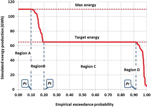
Region A

The system produces excess energy with respect to target $e^{\ast }$, by conveying surplus storage through the turbines, and at the same time the reservoir is spilling, since the conveyance capacity of the penstock is exhausted. In this mode the EPC is flat, given that both the discharge and the gross head are maximized, thus providing the maximum possible energy, i.e.

(18) $e_{\mathrm{m}\mathrm{a}\mathrm{x}}=\psi q\left(z_{\mathrm{m}\mathrm{a}\mathrm{x}}\right)\mathrm{\Delta }t\left(z_{\mathrm{m}\mathrm{a}\mathrm{x}}-z_{\mathrm{d}}\right)$(18)

Region B

The system produces excess energy, bypassing all surplus storage from the turbines, in order to prohibit the generation of spill losses.

Region C

The system operates according to its normal schedule, thus producing the target energy, $e^{\ast }$, which in turn results in a flat EPC. Had we employed the explicit simulation scheme, this region would be approximately flat. The reason is that in explicit simulations, the actual energy is estimated a posteriori, on the basis of the average head across each simulated time interval, while the target volume to release is computed a priori, on the basis of the known head at the beginning of each time step.

Region D

The system produces lower energy than the desirable value, $e^{\ast }$, because of reduced storage and/or head. Using the EPC we can also obtain the average energy production, by integrating the simulated energy vs. percentage of time, the probability of spilling, P_S, the probability of producing excess energy, P_E, and the probability of producing the target energy, P_T, and thus the reliability of the hydroelectric system with respect to the associated target value. By assigning a lower target, its reliability will evidently increase, yet the spread of regions A and B is also expected to increase, thus generating more excess energy and more water losses due to reservoir spilling. On the other hand, by setting a larger target, the region D will expand, thus resulting in more frequent deficits but less water losses. In this context, the shape of the EPC can be used as indicator of the overall performance of a hydroelectric system: the more extended the flat region C, the more spread out the energy production, and thus the more efficient the operation of the system.

4.4 Performance metrics

The twofold operation of hydroelectric reservoirs, i.e. normal and emergent, and the higher price of reliable over surplus energy make it essential to revise the key concept of reliable yield, used in conventional SRY analysis. To begin with, we can outline this metric in a similar manner to water supply reservoirs, namely as the energy value ensured with a given reliability, and estimate it empirically, through EPC analysis. More precisely, the reliable yield of a hydropower system is defined in terms of reliable energy, which requires the assignment of a high probability of exceedance, e.g. 99% on a monthly basis (Koutsoyiannis et al. 2002), to guarantee that this energy will be available even under adverse water conditions (Georgakakos et al. 1997).

Interestingly, while in water supply reservoirs the target water demand and the reliable yield are identical (as the reliable yield is the demand ensured with a given reliability), in hydroelectric reservoirs the target energy, $e^{\ast }$, and the reliable energy, herein symbolized by $e_a$ (where $a$ is the reliability level), are two different concepts. Actually, the target energy dictates the operation of the reservoir, while $e_a$ is a performance metric. In a simulation context, the former is input and the latter is output. To demonstrate this difference, in Fig. 2 we plot $e_a$ as a function of target energy for two reliability levels, namely 95 and 99%, using again as an example the hydroelectric reservoir at Kremasta. This function can be divided into four distinct parts. For low target values, $e_a$ takes a small constant value. For intermediate target energy values, it equals the target one, while after reaching its maximum it drops abruptly. Finally, for large target values, the system produces an overall minimum reliable energy. Apparently, the 99% reliability curve is more conservative than the 95% one, in terms of both minimum and maximum reliable energy. Moreover, the rising limb of the former is very sharp, indicating that the assignment of a very high reliability level makes the detection of the maximized $e_a$ quite sensitive against errors and uncertainties. In particular, the sampling uncertainty of historical data may significantly affect the estimation of $e_a$, which furthermore reveals the usefulness of stochastic approaches.

Figure 2. Plots of alternative energy metrics (95 and 99% reliable energy and monthly average) vs. monthly target energy for the hydroelectric system of Kremasta

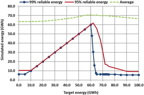
In the same graph (Fig. 2) we also plot the mean monthly energy production, which has been widely used as an overall performance measure in the analysis and optimization of hydroelectric reservoir systems. In contrast to $e_a$, this metric exhibits limited variability against target energy, thus being influenced only little by the management policy of the reservoir. In particular, by not distinguishing energy according to its price, this metric does not follow the obvious deterioration of the reliability of energy production, when assigning unrealistically high production goals, thus providing a misleading picture of the system’s performance. Hence, the optimal performance of a hydroelectric system is much better ensured by maximizing the reliable energy for a reasonably high reliability level. This quantity can be easily obtained by using the simulation scheme of section 4.2 as the underlying model and solving an optimization problem with one control variable, i.e. the target energy.

However, the maximization of $e_a$ may still be insufficient for fully assessing the system’s performance, without also considering the sharing between reliable and surplus energy. Surprisingly, the literature reports limited works clearly distinguishing these two types of energy in a simulation-optimization context (Koutsoyiannis et al. 2002, 2003, Afzali et al. 2008, Li and Qiu 2015, Tsoukalas and Makropoulos 2015, Taghian and Ahmadianfar 2018). On the other hand, retaining water for later hydropower generation, to reduce the overall risk of energy shortage, is a well-known practice, through the concept of hedging rules (e.g. Tayebiyan et al. 2019, Wang et al. 2019), also employed in water supply systems (e.g. Draper and Lund 2004). Nevertheless, the practical question arising is the formulation of an overall metric that also accounts for over- and under-production with respect to the energy target, to be used as alternative or complementary to $e_a$. 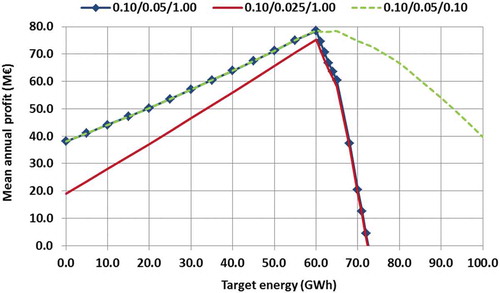This option is offered by introducing a quasi-economic function, reflecting the different market prices reliable against secondary energy and against energy deficits, i.e.

(19) $\begin{array}{rl}& F\left(e^{\ast }\right)=\frac{1}{n}\sum _{t=1}^n\left[c_{\mathrm{f}}\mathrm{m}\mathrm{i}\mathrm{n}\left(e_t,e^{\ast }\right)+c_{\mathrm{s}}\mathrm{m}\mathrm{a}\mathrm{x}\left(0,e_t-e^{\ast }\right)\right.\\ & \left.-c_{\mathrm{d}}\mathrm{m}\mathrm{a}\mathrm{x}\left(0,e^{\ast }-e_t\right)\right]\end{array}$(19)

where $c_{\mathrm{f}}$ is the unit profit for energy production up to the target value $e^{\ast }$, $c_{\mathrm{s}}$ is the unit profit for producing excess energy with respect to $e^{\ast }$, and $c_{\mathrm{d}}$ is a unit penalty for deficits; the latter should be large enough to confirm that the system will produce the target value $e^{\ast }$ with high reliability. We underline that Equation (19)(19) $\begin{array}{rl}& F\left(e^{\ast }\right)=\frac{1}{n}\sum _{t=1}^n\left[c_{\mathrm{f}}\mathrm{m}\mathrm{i}\mathrm{n}\left(e_t,e^{\ast }\right)+c_{\mathrm{s}}\mathrm{m}\mathrm{a}\mathrm{x}\left(0,e_t-e^{\ast }\right)\right.\\ & \left.-c_{\mathrm{d}}\mathrm{m}\mathrm{a}\mathrm{x}\left(0,e^{\ast }-e_t\right)\right]\end{array}$(19) handles reliable and target energy as equivalents. As already discussed, this key assumption is true for a specific range of intermediate target energy values (neither very small, nor very large), which obviously includes the target value that maximizes the overall benefit.

Once again using the Kremasta case, we plot the energy benefit function F versus target $e^{\ast }$ by considering three combinations of unit profit/cost values, i.e. 0.10, 0.05 and 1.0 €/KWh, 0.10, 0.025 and 1.0 €/KWh, and 0.10, 0.05 and 0.10 €/KWh (Fig. 3). In the first setting, we assume a ratio of 2:1 among reliable and secondary energy, and a ratio of 1:10 among production and deficit. The second setting assigns a small benefit for secondary energy generation (4:1 ratio), while the third assigns a very small penalty for deficits (1:1 ratio). It is worth mentioning that all unit profit combinations converge to the same optimal energy target, i.e. 60 GWh/month, which is identical to the target obtained for maximizing the 99% reliable energy (Fig. 2). We observe that for the first two settings the profit function (19) increases linearly with target energy $e^{\ast }$, and after reaching its maximum it drops rapidly. For, by assigning a target energy production even not very far from its optimum results in largely negative profit values, thus penalizing the reduction of reliability further than the optimization of reliable energy itself. On the other hand, a much smoother behaviour is shown with the use of much smaller penalties (third setting), while the profit curve becomes almost flat in the vicinity of the optimum. Nevertheless, the assignment of too-small penalties for energy deficits is not realistic, since it ignores the impacts of shortages in the real-world energy industry.

Figure 3. Plots of alternative profit/penalty metrics vs. monthly target energy for the hydroelectric system of Kremasta (see definitions in the text)

5 Generalized storage-yield analysis for hydroelectric reservoirs

5.1 Problem setting

As discussed so far, the hydroelectric yield can be expressed in terms of the constant energy target that ensures the maximization of the reliable energy $e_a$ or, alternatively, the profit function (19), after assigning reasonable sets of unit profit/cost values. Under the optimization context, the reliable yield of a hydroelectric reservoir with given design characteristics is practically unique, since it can only refer to a very high reliability, while in the case of water supply systems the acceptable reliability range is quite extended. In fact, this describes the trade-off between potential abstractions and frequency of deficits, also applied in multicriteria analyses (e.g. Christofides et al. 2005).

On the other hand, while in the water supply case the reliable yield is determined on the basis of a single design quantity, i.e. the useful storage capacity, the hydroelectric yield is subject to a number of design inputs of the associated simulation model. As explained in section 4.2, these include the minimum and maximum reservoir levels, $z_{\mathrm{m}\mathrm{i}\mathrm{n}}$ and $z_{\mathrm{m}\mathrm{a}\mathrm{x}}$, the downstream elevation, $z_{\mathrm{D}}$, and the characteristic relationships $S=f_1\left(z\right)$, $q=f_2\left(z\right)$ and $\psi =f_3\left(z\right)$. At first glance, the extent of the required information, topographic and hydraulic, makes the problem not only very complicated but also site-specific and thus impractical to generalize. However, under some reasonable assumptions, we can significantly reduce the essential inputs of simulation or express them in terms of representative values (e.g. specific energy), thus providing a generic approach, good for preliminary studies, expressing the hydroelectric yield as a function of few only inputs. In particular, the problem can be fully determined under the following data:

• the time series of inflows arriving from the upstream basin (hydrological input);

• the capacity factor of the hydropower plant (operational input);

• the shape parameter of the elevation-storage function (topographic input);

• the difference in elevation between the outlet and the foot of the dam (design input);

• the useful storage capacity of the reservoir (design input).

The individual assumptions and associated methodologies are discussed in detail next.

5.2 Design discharge as a function of capacity factor

As mentioned in section 4.1, several major design variables of the hydroelectric system are dictated by the role of the power plant in the entire energy mix, which in turn determines the operational schedule of hydropower production. The governing decision is expressed in terms of capacity factor, defined as:

(20) $\mathrm{C}\mathrm{F}=\frac{E_{\mathrm{t}\mathrm{o}\mathrm{t}}}{PT}$(20)

where $E_{\mathrm{t}\mathrm{o}\mathrm{t}}$ is the total energy produced during a sufficient time interval (typically, a year), P is the installed capacity of the power plant, and T is the duration of the given time interval. Under the hypothesis of systematic operation of the turbines at full capacity, the product P T denotes the energy that can potentially be produced during uninterrupted operation, and the ratio $T_{\mathrm{a}}=E_{\mathrm{t}\mathrm{o}\mathrm{t}}/P$ denotes the actual time of operation. On a mean annual basis, the latter can be equivalently expressed in terms of capacity factor, i.e. $T_{\mathrm{a}}=T_{\mathrm{y}\mathrm{e}\mathrm{a}\mathrm{r}}\mathrm{C}\mathrm{F}$ (1 year = 8760 hours).

In the design of large hydroelectric reservoirs, the capacity factor, CF, or, equivalently, the annual time of operation, $T_{\mathrm{a}}$, can be specified a priori, given that the outflows are practically fully regulated. Consequently, this allows us to estimate the design capacity of all conveyance components. In particular, if $V_{\mathrm{a}}$ is the expected (mean) annual water release for energy production, then the discharge capacity is:

(21) $q_0=\frac{V_{\mathrm{a}}}{T_{\mathrm{y}\mathrm{e}\mathrm{a}\mathrm{r}}\mathrm{C}\mathrm{F}}$(21)

For the estimation of the hydroelectric yield via the simulation model of section 4.2, we can use $q_0$ as the upper limit of withdrawals, instead of employing the more accurate yet site-specific hydraulic relationship, i.e. $q=f_2\left(z\right)$. Considering also a single water use, i.e. hydropower production, and minimal losses due to spill (thus a reservoir with a quite large capacity), the mean annual water release can be set equal to the mean annual inflow, as estimated from the available hydrological data.

5.3 Representative value of specific energy

As explained in section 4.2, specific energy, $\psi$, is an overall measure that embeds the hydraulic losses across the water conveyance system as well as the energy losses across the electromechanical components (turbines, generators, transformers). Actually, this varies with discharge and efficiency, which are functions of head. However, the common operation policy of large hydroelectric work implies releasing a constant discharge, also referred to as nominal, which is equal or close to the flow capacity, to ensure the maximization of efficiency. Under this premise, the variation of specific energy with respect to head is very small, which allows the consideration of $\psi$ as a constant property.

To assign a representative value of specific energy, we consider the efficiency and the percentage of hydraulic losses to be normally distributed random variables. In particular, we assign a mean value of 0.90 and 0.05, respectively, and a common standard deviation of 0.01, to describe their expected variability in real-world large hydroelectric systems. In can be easily proved that the derived distribution function of specific energy, which is the product of the two random variables, is also normal, with a mean value of 0.00233 kWh/m⁴ and a small coefficient of variation of only 1.5%. In this context, the specific energy can be handled as a constant, using the aforementioned mean value as representative input property within energy-head-outflow calculations.

5.4 Generalized elevation-storage relationship

The literature reports several attempts to establish generic relationships to link the three characteristic geometrical variables of reservoirs, i.e. elevation, area and storage, through linear or nonlinear equations. To our knowledge, the equations most extensively used are those developed by Lehner et al. (2011) from the Global Reservoir and Dam (GRanD) database. Other researchers provided regional relationships that evidently ensure better results than the global ones, due to geomorphological similarity (van Bemmelen et al. 2016, Adeloye et al. 2019). Nevertheless, such approaches have been mostly applied for dam siting, storage capacity estimations and evaporation adjustment, and not for the simulation of hydroelectric energy.

Herein we present an alternative parameterization, where the storage-elevation function is expressed by means of a sole geomorphological input, using a power-type relationship:

(22) $h\left(S\right)=\lambda S^{\kappa }$(22)

where h is the water depth with respect to a characteristic elevation (in particular, the ground elevation at the foot of the dam), while λ and κ are scale and shape parameters, respectively (we remind the reader that the upper-case symbol S is applied for gross storage, while the lower-case symbol s denotes the active storage). The relationship is not dimensionally homogeneous, and we evaluate it for units of m for h and hm³ for S. For a given reservoir, λ and κ can be empirically derived by fitting Equation (22)(22) $h\left(S\right)=\lambda S^{\kappa }$(22) to local bathymetric data. The straightforward fitting method is regression, providing analytical estimations of λ and κ.

To investigate the variation of water elevation with respect to storage for different reliefs, we used topographic information from 20 large reservoirs in Greece (13 of which are hydroelectric). Summary data, including the optimized “local” parameters λ and κ, are provided in Table 1, while the full data, including the analyses herein, are given as supplementary material. We remark that the local shape parameter values range from 0.318 (Ilarion dam, in the middle course of Aliakmon), to 0.558 (Stratos dam, in the lower course of Achelous). Evidently, the lower the value of κ, the sharper the relief, and thus the faster the increase of elevation with respect to storage (and vice versa).

Table 1. Summary information for the sample of 20 large reservoirs in Greece (hydroelectric reservoirs are marked with *)

Name	Basinarea(km^2)	Min.level (m)	Max.level(m)	Deadvol.(hm^3)	Totalcapacity(hm^3)	Localκ	Localλ	RMSE local (hm^3)	Genericκ	RMSE gen. (hm^3)
Aposelemis	62.4	184.0	216.0	0.9	27.5	0.419	10.47	0.36	0.356	1.82
Evinos	351.9	458.5	505.0	25.0	138.9	0.392	13.75	1.35	0.344	2.50
Gadouras	151.5	95.0	117.5	7.4	67.5	0.341	10.12	0.12	0.370	0.68
Ilarionas*	5005.0	366.0	403.0	166.1	575.2	0.318	14.74	3.81	0.359	4.94
Kastraki*	548.0	142.0	144.2	750.0	800.0	0.408	4.85	0.64	0.400	0.76
Kremasta*	3570.0	227.0	282.0	1000.0	4500.0	0.434	3.15	1.46	0.427	1.33
Marathon	120.0	204.4	224.0	9.4	42.0	0.484	6.21	0.42	0.372	2.03
Mornos	588.1	384.0	435.0	133.9	772.1	0.334	12.44	0.36	0.363	2.02
Mesohora*	633.0	731.0	770.0	132.8	358.0	0.350	16.52	0.79	0.344	0.95
Mouzaki*	139.1	250.0	290.0	28.5	162.9	0.364	13.33	8.93	0.355	4.86
Plastiras*	161.3	776.0	792.0	144.0	507.8	0.380	3.93	0.86	0.437	1.17
Platanovrysi*	10.0	223.5	227.5	71.1	82.8	0.325	19.64	1.23	0.341	1.47
Polyfyto*	5800.0	270.0	291.1	1024.0	2244.0	0.384	5.79	0.33	0.398	0.81
Pournari*	1814.0	100.0	120.0	387.7	736.4	0.448	4.14	0.00	0.390	2.90
Pyli	132.0	310.0	355.0	19.2	125.8	0.362	15.78	1.23	0.344	1.34
Sfikia*	10.0	141.8	146.5	81.0	99.0	0.333	14.70	1.11	0.354	0.72
Smokovo	376.5	331.0	375.0	30.8	230.0	0.333	14.70	1.92	0.354	1.97
Stratos*	202.0	67.0	68.6	60.0	70.2	0.558	1.60	0.28	0.448	0.80
Sykia*	540.0	485.0	550.0	94.0	590.8	0.346	15.61	2.89	0.348	2.83
Thesavros*	4315.5	320.0	380.0	128.9	671.0	0.339	15.44	2.49	0.350	3.08

As illustrated in Fig. 4Fig. 5, the optimized values of λ and κ are well correlated, through a negative power-type law. This enables the application of a more parsimonious formulation of the elevation-storage relationship, where the scale parameter, λ, is expressed as a function of the shape parameter, κ. After testing several parameterizations, we arrived at the following generalized equation:

(23) $h\left(S\right)=a{\left(\kappa -{\kappa }_0\right)}^{-}{S}^{\kappa }$(23)

Figure 4. Scatter plot of shape vs. scale parameters of the elevation-storage function (22), using data from 20 large reservoirs in Greece

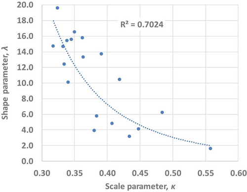
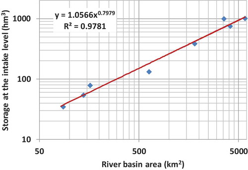
Figure 5. Scatter plot of minimum storage vs. upstream basin area, using data from eight large hydroelectric reservoirs in Greece

where $a$ and $\beta$ are numerical coefficients, and ${\kappa }_0$ is a lower threshold of the shape parameter κ, that has been a priori set equal to ¼ = 0.25. This refers to an extremely steep topography, where the rate of storage increase with respect to elevation is a power function of order 4. Next, the numerical coefficients were estimated together with the individual shape parameters of the 20 reservoirs, by fitting Equation (23)(23) $h\left(S\right)=a{\left(\kappa -{\kappa }_0\right)}^{-}{S}^{\kappa }$(23) to the entire dataset, using as the objective function the sum of the root mean square error (RMSE) values. The optimized expression of the scale parameter was found to be:

(24) $\lambda =0.0386{\left(\kappa -0.25\right)}^{-2.574}$(24)

The adjusted values of $\kappa$ (herein referred to as the generic shape parameter), now ranging from 0.341 to 0.448, are given in Table 1. In almost all cases, the use of the generalized expression ensures a very satisfactory fitting to the real topography, as also indicated by the close values of RMSE with respect to the local approach, i.e. regression. This confirms the suitability of (23) for quantifying the impacts of relief in any kind of reservoir analysis, by only tuning one input, namely the generic shape parameter, κ.

5.5 Other assumptions

The remaining inputs of hydroelectric yield simulations are the characteristic levels $z_{\mathrm{m}\mathrm{i}\mathrm{n}}$, $z_{\mathrm{m}\mathrm{a}\mathrm{x}}$, and $z_{\mathrm{d}}$. The first two are equivalently expressed in terms of minimum and maximum storage, both being essential subjects of reservoir planning. In the general case, $S_{\mathrm{m}\mathrm{i}\mathrm{n}}$ is set at least equal to the volume of sediment that is expected to be deposited into the reservoir during its economic life. However, in hydroelectric reservoirs it is quite usual to put the intake level at a higher elevation, to ensure increased heads. The underlying design problem is far from straightforward, and it is apparently site specific. On the other hand, it is reasonable to assume the upstream basin area is a key explanatory factor of minimum storage, $S_{\mathrm{m}\mathrm{i}\mathrm{n}}$, since it is obviously associated with erosion and sedimentation processes. This hypothesis is strongly supported by the reservoir data provided in Table 1. In particular, by only considering a subset of eight large hydroelectric reservoirs, we established the following empirical relationship:

(25) $S_{\mathrm{m}\mathrm{i}\mathrm{n}}=1.06A^{0.80}$(25)

where $S_{\mathrm{m}\mathrm{i}\mathrm{n}}$ is expressed in hm³ and the upstream area, A, is given in km². As shown in Fig. 5, this very simple relationship makes an excellent fit to the data. We remark that our subset contains only eight out of 20 reservoirs, since from the initial sample we excluded the water supply reservoirs as well as five small hydroelectric ones that are located downstream of head dams, for employing daily up to weekly regulations.

The last input is the downstream level, which is expressed in terms of the elevation difference from the foot of the dam, i.e. $h_{\mathrm{d}}=z_{\mathrm{b}}-z_{\mathrm{d}}$. Therefore, the gross head, which is employed within hydroelectric energy calculations through Equation (12)(12) $e=\psi r\left(z-z_{\mathrm{d}}\right)$(12) , is given by:

(26) $z-z_{\mathrm{d}}=h\left(S\right)-h_{\mathrm{d}}$(26)

where $h\left(S\right)$ is the elevation difference between the actual reservoir level and the foot of the dam, which is estimated by the generalized elevation-storage function (23).

The problem is further simplified by assuming that the power plant is installed at the foot of the dam, while the downstream water level is not affected by river flows or a downstream reservoir, thus $h_{\mathrm{d}}=0$. This assumption is the most conservative and is valid for quite a large portion of real-world hydroelectric systems, which are equipped with reaction turbines. Finally, we also assume that the energy production is not affected by abstractions or regulations made for environmental purposes. In this respect, for a given catchment area, A, shape parameter $\kappa$, and capacity factor, CF, the simulation problem becomes subject to only one design variable, i.e. the active storage capacity, K. This allows us to establish an equivalent storage-reliability-yield analysis for large hydroelectric works, following the rationale of the traditional formulation for water supply reservoirs.

6 Test problems

6.1 Design of experiment

In order to test our methodological framework for a wide range of input data, we employed monthly simulations of a large number of hypothetical reservoirs, receiving their inflows from three hypothetical river basins of the same extent, i.e. 1000 km². In this context, we designed a synthetic experiment by combining:

• Three synthetic inflow time series of 5000 years length (60 000 time steps), generated through a stochastic model on the basis of historical data from three river basins in Greece with different hydroclimatic regimes (see section 6.2);

• Two operational modes, representing the generation of base and peak energy, expressed in terms of capacity factors of 20% and 80%, respectively;

• Seven reservoir geometry patterns (shown in Fig. 6) generated by applying the generalized storage-elevation function (23) with generic shape parameter values $\kappa$ = 0.350, 0.375, 0.400, 0.425, 0.450, 0475 and 0.500, and estimating the associated scale parameters through Equation (24)(24) $\lambda =0.0386{\left(\kappa -0.25\right)}^{-2.574}$(24) .

Figure 6. Plots of reservoir elevation vs. storage as a function of the seven shape parameter values that were applied in simulations

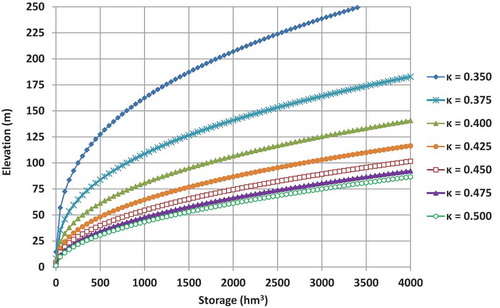
In this respect, we formulated 3 × 2 × 7 = 42 settings of the hydroelectric yield analysis problem, with respect to the useful storage capacity, K. To avoid the generation of extremely large reservoirs, we applied combinations with shape parameters resulting in dam heights and thus heads up to 250 m (only a dozen dams globally exceed this height) and gross storage capacities up to 4000 hm³, which is up to 4 times the mean annual inflow of the wettest basin (see Table 2).

Table 2. Summary information and key statistical characteristics of historical data used for the generation of synthetic inflows; the statistics of synthetic data are shown in parentheses

	Achelous	Evinos	Boeoticos Kephisos
Monitoring site	Kremasta dam	Evivos dam	Karditsa channel
River basin area (km^2)	3570	352	1930
Historical data	October 1966–December 2009	October 1970–November 2018	October 1907–September 2019
Mean annual runoff (mm)	964.5 (958.5)	805.7 (804.6)	191.1 (188.1)
Standard deviation (mm)	235.5 (232.8)	225.8 (223.1)	83.1 (82.0)
Hurst exponent^a	0.85 (0.81)	0.64 (0.66)	0.79 (0.77)

^aThe Hurst exponent, at the annual scale, has been estimated though the method of maximum likelihood (McLeod and Hipel 1978, Tyralis and Koutsoyiannis 2011).

For each K, we sought the target energy ensuring the optimal system performance, by setting as the objective function two alternative probabilistic metrics, i.e. the 99% reliable energy and the expected annual profit (Equation 19(19) $\begin{array}{rl}& F\left(e^{\ast }\right)=\frac{1}{n}\sum _{t=1}^n\left[c_{\mathrm{f}}\mathrm{m}\mathrm{i}\mathrm{n}\left(e_t,e^{\ast }\right)+c_{\mathrm{s}}\mathrm{m}\mathrm{a}\mathrm{x}\left(0,e_t-e^{\ast }\right)\right.\\ & \left.-c_{\mathrm{d}}\mathrm{m}\mathrm{a}\mathrm{x}\left(0,e^{\ast }-e_t\right)\right]\end{array}$(19) ), by setting the recommended unit profit/cost values of 0.10, 0.05 and 1.0 €/KWh, for target energy, excess energy and energy deficits, respectively (see section 4.4). For given (i.e. simulated) sets of monthly energy production and corresponding profit values, the reliable energy was empirically estimated as the 99% percentile, i.e. the 600^th lowest production value, while the expected annual profit was estimated as the empirical mean of the associated profit data. At this point, it is useful to mention that the first statistical metric involves an extreme probability, which is prone to sample uncertainties, thus requiring long simulation horizons, while the profit metric is much more robust and can be accurately estimated even from relatively short datasets.

Apart from the upstream drainage area, other common inputs of the problem were:

• The dead storage that was set equal to $S_{\mathrm{m}\mathrm{i}\mathrm{n}}=$266 hm³, by solving the empirical relationship (26) for the hypothetical drainage area of 1000 km²;

• The specific energy that was set equal to $\psi =$0.00233 kWh/m⁴ (see section 5.3);

• The elevation difference of the outlet level from the foot of the dam, which was set equal to $h_{\mathrm{d}}=0$ (see section 5.5).

6.2 Generation of synthetic inflow data

In order to evaluate the simulation framework against different hydroclimatic conditions, at the same time ensuring a long enough simulation horizon, we followed a stochastic approach. In this context, we generated synthetic inflow time series of 5000 years’ length, which reproduce the stochastic regimes of the observed runoff of three characteristic Greek river basins, i.e. Achelous (upstream of Kremasta dam), Evinos (upstream of the homonymous dam), and Boeoticos Kephisos (at the basin outlet). Summary information about the three flow sites is given in Table 2. The first two datasets (Kremasta, Evinos) were extracted by solving the monthly water balance of the associated reservoirs for the unknown inflows, while the monthly runoff of Boeoticos Kephisos, which is the oldest flow station in Greece (110 years), was estimated on the basis of daily stage observations. Further details about the three basins are provided by Efstratiadis et al. (2014b), Koutsoyiannis et al. (2003) and Nalbantis et al. (2011), respectively.

For monthly data synthesis we employed the modular disaggregation-based stochastic simulation framework by Tsoukalas et al. (2019), as implemented in the R package called AnySim (Tsoukalas et al. 2020), the backbone of which is the notion of Nataf joint distribution, also known as Gaussian copula. This allows for coupling multiple Nataf-based stochastic simulation models to synthesize data that follow specific marginal distributions and correlation structures across multiple temporal scales of interest, and across seasons as well. For this particular study, we configured a scheme that couples two models of this type, one for the annual scale and another for the monthly scale.

Specifically, at the annual time scale we used the Symmetric Moving Average To Anything (SMARTA) model of Tsoukalas et al. (2018b), which implements the symmetric moving average generation mechanism introduced by Koutsoyiannis (2000). For the monthly scale, in contrast, we employed a cyclostationary Nataf-based generation scheme termed Stochastic Periodic Autoregressive To Anything (SPARTA; Tsoukalas et al. 2018a). Both models were combined with the three-parameter Generalized Gamma distribution (Stacy 1962) for modelling the marginal distribution of the parent process (at monthly and annual scales), while SMARTA was parameterized using the two-parameter Cauchy autocorrelation structure (Koutsoyiannis 2000, Tsoukalas et al. 2018b), which is suitable for the description of short- or long-range dependent processes (e.g. processes with Hurst exponent exceeding 0.50; see Table 2). The combined scheme reproduces the seasonal and annual distributional and dependence properties of the historical data, also including the Hurst phenomenon.

6.3 Results

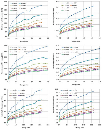
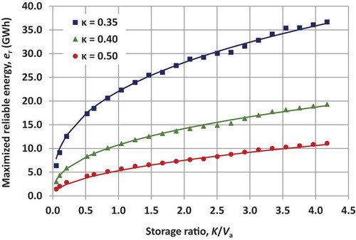
The main results of the simulation-optimization analyses are shown in Figs 7 and Figure 8, which illustrate the storage-yield relationships for CF values of 80 and 20%, respectively. On each graph we plot the maximized values of 99% reliable energy and the maximized mean annual profit function (19), with respect to storage ratio (i.e. reservoir capacity, $K$, divided by mean annual inflow, $V_{\mathrm{a}}$) and reservoir geometry, expressed in terms of the generic shape parameter, κ. As expected, by setting the low capacity factor, i.e. CF = 20%, thus operating the power station for peak energy production, the expected profit increases with respect to the base energy scenarios (CF = 80%), while the differences in terms of maximized reliable energy are quite small.

Figure 7. Plots of maximized 99% reliable energy (left) and maximized profit as a function of the storage ratio and the shape parameter, κ, for capacity factor (CF) = 80% (upper panel: Achelous; middle panel: Evinos; lower panel: Boeoticos Kephisos)

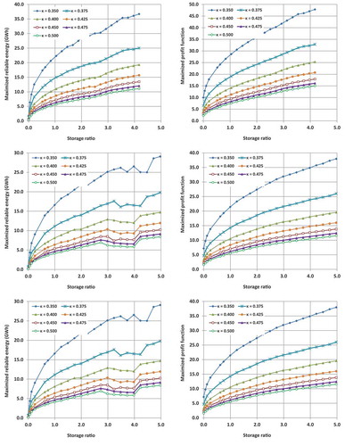
Figure 8. Plots of maximized 99% reliable energy (left) and maximized profit as a function of the storage ratio and the shape parameter, κ, for capacity factor (CF) = 20% (upper panels: Achelous; middle panels: Evinos; lower panels: Boeoticos Kephisos)

Nevertheless, for all synthetic runoff sets and operation mode scenarios, common findings are the following:

• The maximized 99% reliable energy, i.e. the objective function, and the control variable of the associated optimization problem, i.e. the target energy, are identical, thus confirming the preliminary findings of section 4.4.

• The sole exception is the case of zero storage capacity, for which the derived reliable energy is systematically higher than the corresponding target. This outcome is reasonable, since due to the lack of regulation capacity, the target energy should be small enough to avoid energy deficits that are due to low summer flows. In particular, in the case of Boeoticos Kephisos, considered representative of a quite dry flow regime, the target energy is close to zero.

• In general, the maximization of 99% reliable energy and the maximization of mean annual profit are ensured for the same target power value, which is also in line with the conclusions drawn in section 4.4. Few and rather small differences only appear for relatively small storage capacities. This important finding allows for handling both metrics as equivalent to the reliable yield in hydroelectricity.

Although the two metrics converge to the same optimal management policy, expressed in terms of target power production, the mean annual profit is less prone to statistical uncertainties induced by the sample size. As shown in most graphs, the empirically derived reliable energy curve is quite irregular, while the mean profit curve is smooth. In fact, the estimation of extreme probabilistic quantities, such as reliable energy, would require a much larger simulation horizon to ensure satisfactory accuracy. On the other hand, the mean annual profit is much more easily stabilized, given that it expresses a first-order moment. We remark that the statistical accuracy of simulation outputs is affected not only by the length of the simulation but also by the long‐term persistence, which is a key property of hydroclimatic processes (Koutsoyiannis and Montanari 2007).

6.4 Reliable energy as a function of reservoir storage and geometry

As shown in Figs 7 and Figure 8, the hydroelectric yield, expressed either by means of 99% reliable energy or in profit terms, can be approximated by a power-type function of the storage ratio, $K/V_{\mathrm{a}}$. By considering the first metric we get:

(27) $e_a=\zeta {\left(\frac{K}{V_{\mathrm{a}}}\right)}^{\theta }$(27)

where parameters ζ and θ can be straightforwardly extracted via regression.

In Table 3 we show the optimized values of ζ and θ for each site and for CF = 80%, against the seven storage-elevation scenarios, which are expressed in terms of the shape parameter κ of the generalized storage function. Both quantities are highly correlated with κ. In particular, ζ is a decreasing function of κ, while the exponent θ is almost perfectly approximated by a linear function of κ. Similar conclusions are extracted for CF = 20%.

Table 3. Fitting of Equation (27)(27) $e_a=\zeta {\left(\frac{K}{V_{\mathrm{a}}}\right)}^{\theta }$(27) to simulated data at three river sites, for CF = 80%

Shape parameter, κ	Achelous		Evinos		Boeoticos Kephisos
	ζ	θ	ζ	θ	ζ	θ
0.350	21.524	0.383	16.163	0.399	2.088	0.329
0.375	14.381	0.393	10.763	0.410	1.359	0.345
0.400	10.657	0.409	7.936	0.418	0.982	0.362
0.425	8.484	0.421	6.284	0.430	0.765	0.378
0.450	7.105	0.434	5.266	0.440	0.625	0.395
0.475	6.227	0.446	4.585	0.450	0.534	0.413
0.500	5.612	0.459	4.134	0.461	0.473	0.428
Correlation with κ	−0.916	0.999	−0.916	0.992	−0.916	0.967

This interesting outcome triggered us to look for a fully generic relationship, expressing the maximized reliable energy as a function of reservoir size and geometry, given in terms of the storage ratio, $K/V_{\mathrm{a}}$, and the generic shape parameter, κ, respectively. After our investigations, we arrived at the following expression:

(28) $e_{\alpha }=\frac{1}{\beta \kappa -\delta }{\left(\frac{K}{V_{\mathrm{a}}}\right)}^{\kappa }$(28)

The optimized values for the two parameters of Equation (28)(28) $e_{\alpha }=\frac{1}{\beta \kappa -\delta }{\left(\frac{K}{V_{\mathrm{a}}}\right)}^{\kappa }$(28) are given in Table 4. These are derived by minimizing the total square error between the simulated reliable energy data of Fig. 7 and the theoretical relationship (28). In all cases the fitting is almost perfect, as illustrated in the example of Fig. 9. Apparently, the two local parameters β and δ of Equation (28)(28) $e_{\alpha }=\frac{1}{\beta \kappa -\delta }{\left(\frac{K}{V_{\mathrm{a}}}\right)}^{\kappa }$(28) are associated with the hydrological regime of each site of interest. For instance, both parameters decrease with mean annual runoff, while their ratio, $\delta /\beta$, remains practically constant at all sites, i.e. 0.30. Obviously, our sample is too small to extract safe conclusions, which would require us to solve the problem for many inflow datasets, with varying stochastic behaviour, to investigate whether these parameters can be linked with summary hydroclimatic indices. We remark that similar regionalization attempts have been quite common for water supply reservoirs, carried out by means of regression formulae explaining SRY on the basis of mean annual statistical characteristics of inflows, such as standard deviation and skewness (e.g. Koutsoyiannis 2005a, McMahon et al. 2007a).

Table 4. Optimized parameters of the generalized relationship (28) for the three river sites

Parameter	Achelous	Evinos	Boeoticos Kephisos
β	0.955	1.316	12.652
δ	0.289	0.401	3.931

Figure 9. Fitting of generalized relationship (28), illustrated with solid lines, to empirically derived (simulated) reliable energy against the storage ratio at Achelous, for three characteristic reservoir geometries

7 Summary and discussion

While SRY analysis is a well-established tool for reservoir sizing, its applicability has been limited to systems serving consumptive water uses. A similar approach for the preliminary design of hydropower systems is lacking, which is due, in our viewpoint, to two key reasons.

First, the crucial concepts of yield and reliability are not well defined in hydroelectricity, where the water demand is dictated by the energy demand and thus the yield must be determined in terms of energy production. Since such systems allow for the generation of excess energy with respect to the corresponding demand, by passing surplus storage from the turbines, the yield can be considered as a two-fold component, i.e. a target rate to be guaranteed with minimal risk and the excess production above this value. These are referred to as reliable and secondary energy, respectively. In fact, reliable energy is a probabilistic quantity, which can be theoretically derived from the distribution function of power production data. Empirically, this can be easily determined by means of an extreme quantile of the energy-probability curve, e.g. the energy produced at least 99% of time. In this respect, reliable energy is the equivalent of the reliable yield ensured from water supply reservoirs.

The second obstacle in establishing SRY relationships for hydroelectric reservoirs is rather technical, since it originates from the inherent complexities of the underlying processes, mainly the dependence on local geometry and the nonlinearities induced by the storage-head-energy transformations. Our research indicates that the site-specific properties of a hydroelectric system can be effectively parameterized even through a single parameter, namely the shape parameter of the storage-elevation relationship. After also employing a few reasonable simplifications, which are acceptable for a preliminary study, the water balance dynamics of a hydroelectric reservoir that is expected to operate under a specific capacity factor are well approximated by using only two input properties, i.e. the storage capacity and the shape parameter, both characteristics of reservoir geometry.

In this respect, we demonstrated that the equivalent “storage-reliability-yield” problem for hydroelectric reservoirs involves three interdependent quantities, in addition to reliability per se, namely the storage capacity, the geometry, and the reliable energy. For this problem, we proposed a robust stochastic simulation-optimization framework that allows us to employ comprehensive screening analyses of the hydroelectric yield, on the basis of monthly runoff series. Our pilot investigations at three river sites in Greece exhibiting different hydrological regimes indicate that it is possible to extract generic empirical formulae that link reservoir storage, topography and reliable energy with summary runoff statistics.

In our analyses we also demonstrate that the maximization of this yield is achieved by using either the reliable energy per se or a quasi-economic (profit) function, which accounts for sharing between the expected values of reliable energy, secondary energy and energy deficits. The two approaches converge to a practically identical target energy value, which is the sole control variable of the underlying optimization problem. However, the profit function seems much less sensitive to sample uncertainties, since it is expressed in terms of first-order moments, while the reliable energy function requires the empirical estimation of an extreme statistical metric, i.e. the energy produced with 99% reliability. Nevertheless, this also reveals the irreplaceable role of the stochastic approach, which allows, among other things, for handling sampling uncertainties that are unavoidable when using historical runoff data in simulations.

There remain several open questions to be addressed in the next research steps. First, the generalized storage-elevation function (23), which describes the reservoir geometry in terms of a generic shape parameter $\kappa$, should be fitted to a much larger sample of reservoirs, to better identify the empirical relationship (24). This will allow us to employ this equation not only in the context of theoretical simulation analyses (i.e. for sampling different reservoir storages), but also for preliminary design purposes in areas with limited topographic data.

Next, the whole framework must be also tested with an extended set of streamflow properties, in order to validate the theoretical relationship (28). Another useful task will be to evaluate the simulation results with actual reservoir data and the outcomes from real-world design studies. A final research option is the assessment of the hydroelectric yield with respect to the stochastic structure of the underlying runoff process. This will also allow us to outline the specifications of the synthetic time series generator, which is a key component of our framework. Our ongoing research outcomes regarding this important issue will be reported in due course.

Data availability

Reservoir data have been mainly retrieved from the summary report published by the Greek Committee on Large Dams (2013).

Acknowledgments

The overall idea for this research originates from a simulation exercise assigned to our students who attend the course on Renewable Energy and Hydroelectric Works in the School of Civil Engineering at the National Technical University of Athens. The challenges reported so far have prompted us to provide a theoretical basis for the underlying problem, initially introduced for educational reasons. We are grateful to the Associate Editor, Krzysztof Kochanek, who coordinated the review procedure, and the two anonymous reviewers for their fruitful comments and suggestions that helped us to improve this article.

Disclosure statement

No potential conflict of interest was reported by the authors.

Supplementary material

Supplemental data for this article can be accessed here.

References

- Adeloye, A.J., 2009. Multiple linear regression and artificial neural networks models for generalized reservoir storage–yield–reliability function for reservoir planning. Journal of Hydrologic Engineering, 14 (7), 731–738. doi:10.1016/j.jhydrol.2005.10.033
- Adeloye, A.J., et al., 2015. Stochastic assessment of Phien generalized reservoir storage–yield–probability models using global runoff data records. Journal of Hydrology, 529 (3), 1433–1441. doi:10.1016/j.jhydrol.2015.08.038
- Adeloye, A.J., et al., 2019. Height–area–storage functional models for evaporation-loss inclusion in reservoir-planning analysis. Water, 11, 1413. doi:10.3390/w11071413
- Adeloye, A.J. and De Munari, A., 2006. Artificial neural network based generalised storage-yield-reliability models using the Levenberg-Marquardt algorithm. Journal of Hydrology, 326 (1), 215–230. doi:10.1016/j.jhydrol.2005.10.033
- Adeloye, A.J., Pal, S., and O’Neill, M., 2010. Generalised storage-yield-reliability modelling: independent validation of the Vogel–Stedinger (V–S) model using a Monte Carlo simulation approach. Journal of Hydrology, 388 (3–4), 234–240. doi:10.1016/j.jhydrol.2010.04.043
- Afzali, R., Mousavi, S., and Ghaheri, A., 2008. Reliability-based simulation-optimization model for multireservoir hydropower systems operations: Khersan experience. Journal of Water Resources Planning and Management, 134 (1), 24–33. doi:10.1061/(ASCE)0733-9496(2008)134:1(24)
- ASCE, 1995. Glossary of hydropower terms. In: Guidelines for design of intakes for hydroelectric plants, energy division of the American society of civil engineers. Committee on Hydropower Intakes. New York, NY: American Society of Civil Engineers.
- Celeste, A.B., 2015. Reservoir design optimization incorporating performance indices. Water Resources Management, 29 (12), 4305–4318. doi:10.1007/s11269-015-1061-4
- Christofides, A., et al., 2005. Resolving conflicting objectives in the management of the Plastiras Lake: can we quantify beauty? Hydrology and Earth System Sciences, 9 (5), 507–515. doi:10.5194/hess-9-507-2005.
- Draper, A.J. and Lund, J.R., 2004. Optimal hedging and carryover storage value. Journal of Water Resources Planning and Management, 130 (1), 83–87. doi:10.1061/(ASCE)0733-9496(2004)130:1(83)
- Efstratiadis, A., et al., 2014a. A multivariate stochastic model for the generation of synthetic time series at multiple time scales reproducing long-term persistence. Environmental Modelling and Software, 62, 139–152. doi:10.1016/j.envsoft.2014.08.017
- Efstratiadis, A., et al., 2014b. Assessment of environmental flows under limited data availability – case study of the Acheloos River, Greece. Hydrological Sciences Journal, 59 (3–4), 731–750. doi:10.1080/02626667.2013.804625
- Fletcher, S. and Ponnambalam, K., 1996. Estimation of reservoir yield and storage distribution using moments analysis. Journal of Hydrology, 182, 259–275. doi:10.1016/201C-1694(95)02946-X
- Georgakakos, A., Yao, H., and Yu, Y., 1997. Control models for hydroelectric energy optimization. Water Resources Research, 33 (10), 2367–2379. doi:10.1029/97WR01714
- Gould, B., 1961. Statistical methods for estimating the design capacity of dams. Journal of the Institution for Engineers, Australia, 33 (12), 405–415.
- Greek Committee on Large Dams, 2013. The dams of Greece. Available from: http://www.eeft.gr/Fragmata_Elladas_201311.pdf (accessed 16 January 2021).
- Hamed, K., 2012. A probabilistic approach to calculating the reliability of over-year storage reservoirs with persistent Gaussian inflow. Journal of Hydrology, 448-449, 93–99. doi:10.1016/j.jhydrol.2012.04.051
- Harr, M.E., 1987. Reliability-based design in civil engineering. McGraw-Hill.
- Hashimoto, T., Stedinger, J.R., and Loucks, D.P., 1982. Reliability, resiliency and vulnerability criteria for water resource system performance evaluation. Water Resources Research, 18 (1), 14–20. doi:10.1029/WR018i001p00014
- Hatamkhani, A., Moridi, A., and Yazdi, J., 2019. A simulation – optimization models for multi-reservoir hydropower systems design at watershed scale. Renewable Energy. doi:10.1016/j.renene.2019.12.055
- Hazen, A., 1914. Storage to be provided in impounding reservoirs for municipal water supply. Transactions of the American Society of Civil Engineers, 77, 1539–1640.
- Klemeš, V., 1987. One hundred years of applied storage reservoir theory. Water Resources Management, 1, 159–175. doi:10.1007/BF00429941
- Koutsoyiannis, D., 2000. A generalized mathematical framework for stochastic simulation and forecast of hydrologic time series. Water Resources Research, 36 (6), 1519–1533. doi:10.1029/2000WR900044
- Koutsoyiannis, D., 2002. The Hurst phenomenon and fractional Gaussian noise made easy. Hydrological Sciences Journal, 47 (4), 573–595. doi:10.1080/02626660209492961
- Koutsoyiannis, D., et al., 2003. A decision support system for the management of the water resource system of Athens. Physics and Chemistry of the Earth, 28 (14–15), 599–609. doi:10.1016/S1474-7065(03)00106-2
- Koutsoyiannis, D., 2005a. Reliability concepts in reservoir design. In: J.H. Lehr and J. Keeley, eds. Water encyclopedia, Vol. 4, surface and agricultural water. New York: Wiley, 259–265. doi:10.1002/047147844X.sw776
- Koutsoyiannis, D., 2005b. Stochastic simulation of hydrosystems. In: J.H. Lehr and J. Keeley, eds. Water encyclopedia, Vol. 4, Surface and agricultural water. New York: Wiley, 421–430. doi:10.1002/047147844X.sw913
- Koutsoyiannis, D., et al., 2009. Climate, hydrology, energy, water: recognizing uncertainty and seeking sustainability. Hydrology and Earth System Sciences, 13, 247–257. doi:10.5194/hess-13-247-2009
- Koutsoyiannis, D., 2011. Hurst-Kolmogorov dynamics and uncertainty. Journal of the American Water Resources Association, 47 (3), 481–495. doi:10.1111/j.1752-1688.2011.00543.x
- Koutsoyiannis, D., 2019. Knowable moments for high-order stochastic characterization and modelling of hydrological processes. Hydrological Sciences Journal, 64 (1), 19–33. doi:10.1080/02626667.2018.1556794
- Koutsoyiannis, D., 2020. Simple stochastic simulation of time irreversible and reversible processes. Hydrological Sciences Journal, 65 (4), 536–551. doi:10.1080/02626667.2019.1705302
- Koutsoyiannis, D. and Economou, A., 2003. Evaluation of the parameterization-simulation-optimization approach for the control of reservoir systems. Water Resources Research, 39 (6), 1170. doi:10.1029/2003WR002148
- Koutsoyiannis, D., Efstratiadis, A., and Karavokiros, G., 2002. A decision support tool for the management of multi-reservoir systems. Journal of the American Water Resources Association, 38 (4), 945–958. doi:10.1111/j.1752-1688.2002.tb05536.x
- Koutsoyiannis, D. and Montanari, A., 2007. Statistical analysis of hydroclimatic time series: uncertainty and insights. Water Resources Research, 43 (5), W05429. doi:10.1029/2006WR005592
- Kritskiy, S.N. and Menkel, M.F., 1935. Long-term streamflow regulation (in Russian), Gidrorekhn. Stroit, 11, 3–10.
- Kritskiy, S.N. and Menkel, M.F., 1940. Generalized methods for runoff control computations based on mathematical statistics. Journal of Hydrology, 172, 365–377, 1995 (translated by V. Klemes from the Russian original “‘Obobshchennye priemy rascheta regulirovaniya stoka na osnove matematicheskoy statistiki”, Gidrotekh. Stroit., 2: 19-24, 1940). doi:10.1016/0022-1694(95)02731-4
- Kuria, F.W. and Vogel, R.M., 2014. Global storage-reliability-yield relationships for water supply reservoirs. Water Resources Management, 29 (5), 1591–1605. doi:10.1007/s11269-014-0896-4
- Lehner, B., et al., 2011. High resolution mapping of the world’s reservoirs and dams for sustainable river-flow management. Frontiers in Ecology and the Environment, 9 (9), 494–502. doi:10.1890/100125
- Lele, S.M., 1987. Improved algorithms for reservoir capacity calculation incorporating storage-dependent losses and reliability norm. Water Resources Research, 23 (10), 1819–1823. doi:10.1029/WR023i010p01819
- Li, -F.-F. and Qiu, J., 2015. Multi-objective reservoir optimization balancing energy generation and firm power. Energies, 8 (7), 6962–6976. doi:10.3390/en8076962
- Mamassis, N., et al., 2021. Water and energy. In: J.J. Bogardi, et al., eds. Handbook of water resources management: discourses, concepts and examples. Cham, Switzerland: Springer. doi:10.1007/978-3-030-60147-8
- Matalas, N. C., & Wallis, J. R. (1976). Generation of synthetic flow sequences. In: A. K. Biswas, ed. Systems Approach to Water Management. New York, NY: McGraw-Hill.
- Mays, L.W. and Tung, Y.-K., 1992. Hydrosystems engineering and management. McGraw-Hill: New York.
- McLeod, I. and Hipel, K.W., 1978. Simulation procedures for Box-Jenkins models. Water Resources Research, 14 (5), 969–975. doi:10.1029/WR014i005p00969
- McMahon, T.A., et al., 2007a. Revisiting reservoir storage-yield relationships using a global streamflow database. Advances in Water Resources, 30 (8), 1858–1872. doi:10.1016/j.advwatres.2007.02.003
- McMahon, T.A., et al., 2007b. Review of Gould–Dincer reservoir storage–yield–reliability estimates. Advances in Water Resources, 30 (9), 1873–1882. doi:10.1016/j.advwatres.2007.02.004
- McMahon, T.A., et al., 2007c. Global streamflows – part 2: reservoir storage–yield performance. Journal of Hydrology, 347 (3–4), 260–271. doi:10.1016/j.jhydrol.2007.09.021
- McMahon, T.A., Adeloye, A.J., and Zhou, S.-L., 2006. Understanding performance measures of reservoirs. Journal of Hydrology, 324 (1–4), 359–382. doi:10.1016/j.jhydrol.2005.09.030
- Moran, P.A.P., 1959. The Theory of Storage. London: Methuen.
- Nalbantis, I., et al., 2011. Holistic versus monomeric strategies for hydrological modelling of human-modified hydrosystems. Hydrology and Earth System Sciences, 15, 743–758. doi:10.5194/hess-15-743-2011
- Pegram, G.G.S., 1980. On reservoir reliability. Journal of Hydrology, 47 (3–4), 269–296. doi:10.1016/0022-1694(80)90097-9
- Phien, H.N., 1993. Reservoir storage capacity with gamma inflows. Journal of Hydrology, 146 (1), 383–389. doi:10.1016/0022-1694(93)90285-H.
- Piao, M.J., Li, Y.P., and Huang, G.H., 2014. Development of a stochastic simulation–optimization model for planning electric power systems – a case study of Shanghai, China. Energy Conversion and Management, 86, 111–124. doi:10.1016/j.enconman.2014.05.011
- Pleshkov, Y.F., 1939. Rapid and accurate computations for storage reservoirs (in Russian). Gidrotekhn. Slroit., 6.
- ReVelle, C., 1999. Optimizing reservoir resources: including a new model for reservoir reliability. New York, NY: John Wiley & Sons.
- Ripley, B.D., 1987. Stochastic Simulation. New York, NY: Wiley Series in Probability and Statistics.
- Rippl, W., 1883. The capacity of storage reservoirs for water supply. Proceedings of the Institution of Civil Engineers, 71, 270–278.
- Savarenskiy, A.D., 1940. A method for runoff control computation. Journal of Hydrology, 172, 355–363, 1995 (translated by V. Klemes from the Russian original “Metod rascheta regulirovaniya stoka, Gidrotekh. Stroit., 2: 24-28, 1940). doi:10.1016/0022-1694(94)02730-Y
- Silva, A.T. and Portela, M.M., 2013. Stochastic assessment of reservoir storage-yield relationships in Portugal. Journal of Hydrologic Engineering, 18 (5), 567–575. doi:10.1061/(ASCE)HE.1943-5584.0000650
- Sivapragasam, C., et al., 2003. Modeling evaporation-seepage losses for reservoir water balance in semi-arid regions. Water Resources Management, 23, 853. doi:10.1007/s11269-008-9303-3
- Stacy, E.W., 1962. A generalization of the gamma distribution. The Annals of Mathematical Statistics, 33 (3), 1187–1192. doi:10.1214/aoms/1177704481
- Sudler, C., 1927. Storage required for the regulation of streamflow. Transactions of the American Society of Civil Engineers, 91, 622–660.
- Taghian, M. and Ahmadianfar, J., 2018. Maximizing the firm energy yield preserving total energy generation via an optimal reservoir operation. Water Resources Management, 32 (1), 141–154. doi:10.1007/s11269-017-1800-9
- Tayebiyan, A., et al., 2019. Comparison of optimal hedging policies for hydropower reservoir system operation. Water, 11 (1), 121. doi:10.3390/w11010121
- Tsoukalas, I., Efstratiadis, A., and Makropoulos, C., 2018a. Stochastic periodic autoregressive to anything (SPARTA): modelling and simulation of cyclostationary processes with arbitrary marginal distributions. Water Resources Research, 54 (1), 161–185, WRCR23047. doi:10.1002/2017WR021394
- Tsoukalas, I., Efstratiadis, A., and Makropoulos, C., 2019. Building a puzzle to solve a riddle: a multi-scale disaggregation approach for multivariate stochastic processes with any marginal distribution and correlation structure. Journal of Hydrology, 575, 354–380. doi:10.1016/j.jhydrol.2019.05.017
- Tsoukalas, I., Kossieris, P., and Makropoulos, C., 2020. Simulation of non-Gaussian correlated random variables, stochastic processes and random fields: introducing the anySim R-package for environmental applications and beyond. Water, 12 (6), 1645. doi:10.3390/w12061645
- Tsoukalas, I. and Makropoulos, C., 2015. A surrogate based optimization approach for the development of uncertainty-aware reservoir operational rules: the case of Nestos hydrosystem. Water Resources Management, 29 (13), 4719–4734. doi:10.1007/s11269-015-1086-8
- Tsoukalas, I., Makropoulos, C., and Koutsoyiannis, D., 2018b. Simulation of stochastic processes exhibiting any-range dependence and arbitrary marginal distributions. Water Resources Research, 54 (11), 9484–9513. doi:10.1029/2017WR022462
- Tyralis, H. and Koutsoyiannis, D., 2011. Simultaneous estimation of the parameters of the Hurst-Kolmogorov stochastic process. Stochastic Environmental Research and Risk Assessment, 25 (1), 21–33. doi:10.1007/s00477-010-0408-x
- van Bemmelen, C.W.T., et al., 2016. Determining water reservoir characteristics with global elevation data. Geophysical Research Letters, 43 (21), 11278–11286. doi:10.1002/2016GL069816
- Vogel, R.M. and Bolognese, R.A., 1995. Storage‐reliability‐resilience‐yield relations for over‐year water supply systems. Water Resources Research, 31 (3), 645–654. doi:10.1029/94WR02972
- Vogel, R.M., Fennessey, N.M., and Bolognese, R.A., 1995. Storage-reliability-resilience-yield relations for Northeastern United States. Journal of Water Resources Planning and Management, 121 (5), 365–374. doi:10.1061/(ASCE)0733-9496(1995)121:5(365)
- Vogel, R.M. and Stedinger, J.R., 1987. Generalized storage-reliability-yield relationships. Journal of Hydrology, 89 (3–4), 303–327. doi:10.1016/0022-1694(87)90184-3
- Wang, J., et al., 2019. Optimal hedging for hydropower operation and end-of-year carryover storage values. Journal of Water Resources Planning and Management, 145 (4), 04019003. doi:10.1061/(ASCE)WR.1943-5452.0001046
- Xie, J., Annandale, G.W., and Wu, B., 2010. Reservoir capacity – potential power generation –reliability estimation based on Gould-Dincer approach. Proceedings of the 34th World Congress of the International Association for Hydro-Environment Research and Engineering, Australia.
- Xie, J., Wu, B., and Annandale, G.W., 2013. Rapid reservoir storage–based benefit calculations. Journal of Water Resources Planning and Management, 139 (6), 712–722. doi:10.1061/(ASCE)WR.1943-5452.0000312
- Xu, J., Ni, T., and Zheng, B., 2015. Hydropower development trends from a technological paradigm perspective. Energy Conversion and Management, 90, 195–206. doi:10.1016/j.enconman.2014.11.016