Uncertainty of potential evapotranspiration modelling in climate change impact studies on low flows in North America

ABSTRACT

This study investigates the uncertainty in hydroclimatic modelling chain components on future changes in potential evapotranspiration, specially on low flows, at the watershed scale. A large domain covering 2080 watersheds located in Canada, the United States and Mexico is studied. The outputs from eight global climate models are post-processed using two methods to produce climate scenarios that drive 10 temperature- and radiation-based potential evapotranspiration (PET) formulas and three lumped conceptual hydrological models, under representative concentration pathways (RCP) 4.5 and 8.5 and for the future periods 2041–2070 and 2071–2100. All simulated results show an increase in PET and a decrease in low flows, computed through three statistical metrics. Based on the results, we advise the use of multiple hydrological model–PET formula combinations when investigating the impact of climate change on low flows. This study provides an assessment of the contribution of potential evapotranspiration formulas to uncertainty throughout the modelling chain.

KEYWORDS:

• evapotranspiration
• hydrological modelling
• climate change
• low flows
• uncertainty

Editor A. Fiori Associate Editor N. Malamos

1 Introduction

In the context of climate change, an increase in the frequency and intensity of extreme hydrological events, such as droughts, is expected according to the last report from the Intergovernmental Panel on Climate Change (IPCC 2014) and to recent studies (e.g. Zhao et al. 2020). More severe and extended low-flow periods will affect the quantity and quality of water resources. These events especially impact water management, water availability and public safety.

Changes in the water cycle are expected to occur due to climate change, and key processes such as evapotranspiration (ET) will be affected (Anctil et al. 2012, Ricard and Anctil 2019). ET plays an important role in the hydrology of watersheds, in particular under warm and dry conditions involved in low-flow periods. Together with the lack of precipitation, ET impacts the water quantities available for runoff and thus directly influences the streamflow.

ET is the volume of water returned to the atmosphere and results from a combination of plant transpiration with water and soil evaporation. It is limited by actual atmospheric conditions (relative humidity, incoming radiation, wind speed, air temperature) and soil water availability. Potential evapotranspiration (PET) is the maximum volume of water apt to return to the atmosphere without considering any constraint on water availability (Oudin 2004, McMahon et al. 2016). As ET is a rather complex process and thus expensive to measure, empirical formulas are used to estimate PET, which can then be used in hydrological modelling to estimate actual evapotranspiration (AET) through PET and water availability computation at each time step. PET is either an input to hydrological models or is determined inside these models as a function of meteorological input data. The PET process often absorbs errors during hydrological calibration in order to close the water balance and to obtain efficient simulated outflows (Beven 2001, Minville et al. 2014).

PET methods are generally separated into five groups (Xu and Singh 2002, Anctil et al. 2012): (1) water balance, (2) mass transfer, (3) combinatorial, (4) radiation-based and (5) temperature-based formulas. Oudin et al. (2005a, 2005b) studied 308 watersheds located in the United States, France and Australia. They concluded that simpler methods (radiation-based and temperature-based) are as effective as more complex methods (combinatorial) and that the performance of hydrological models can even be improved with simpler methods. But these studies were carried out under historical climate conditions and therefore did not take climate change into account.

While most PET formulas can perform similarly well under historical conditions, they have different climate sensitivities and therefore generate uncertainty regarding water availability under changed climate conditions, which needs to be assessed. Kingston et al. (2009) investigated the impact of a 2°C increase on PET change at global scale using six PET formulas and outputs from five global climate models (GCMs). All of the PET formulas predicted an increase in PET, but with differences among the results reaching more than 100% – up to 700% in some cases.

When carrying climate change impact studies in a hydrological modelling context, the key problem is to understand the sensitivity of PET in the uncertainty cascade from the hydroclimatic modelling chain (Kirchner 2006).

Seiller and Anctil (2016) provided some answers by analysing the sensitivity of 24 PET formulations (combinational, temperature-based and radiation-based) using a 20-member ensemble of hydrological models on two contrasting watersheds in Canada and Germany. They found that the conditional calibration of the hydrological model to a PET formulation reduced the impact of PET as the parameter set compensated for differences in PET to close the mass balance. However, for both watersheds, the PET formulas clearly influence the streamflow projections under changed climate conditions and generate a large spread of responses reflecting their contribution to uncertainty along the hydroclimatic modelling chain. Seiller and Anctil (2016) conclude their paper with ideas for future research, namely regarding three elements that could lead to deeper understanding of PET’s role in hydrological impact studies:

1. Perform a study on a larger scale, with a variety of different watersheds, to attempt to generalyse the results;

2. Modify land-use and physical properties, rather than just the meteorological forcing data, during modelling; and

3. Integrate their framework into a larger study, including upstream elements such as climate models and bias correction methods that could give a better sense of PET sensitivity in the overall climate change impact assessment.

In this study, we attempt to extend Seiller and Anctil’s (2016) work by targeting points 1 and 3. Point number 2, while interesting from a scientific point of view, is much more complex to implement and is not compatible with an approach using lumped modelling.

At mid latitudes, ET represents on average half of annual precipitation depth, and in tropical and more arid environments, this proportion can reach values close to 100%. Consequently, the main objective of this study is to evaluate the contribution of PET formulas to uncertainty in the full modelling chain of low flows in the context of climate change, in Canadian, US and Mexican watersheds. Secondary objectives include better assessing the risks during low-flow periods and evaluating the trends in hydrological indices such as low flows in the changing climate.

2 Study area and data

Water availability greatly varies in North America depending on the local climate and topography. While most of Canada has access to good-quality water in large quantities, several North American regions are subject to water stresses. Since PET is directly related to watershed climatic conditions, this study makes use of a large quantity of watersheds from different climatic zones, thus increasing the robustness of the results.

The study area encompasses 2080 watersheds of North America, including 235 watersheds in Canada, 1825 watersheds in the United States and 20 watersheds in Mexico. The locations of the watersheds are presented in Fig. 1.

Figure 1. Location of the 2080 watersheds in North America

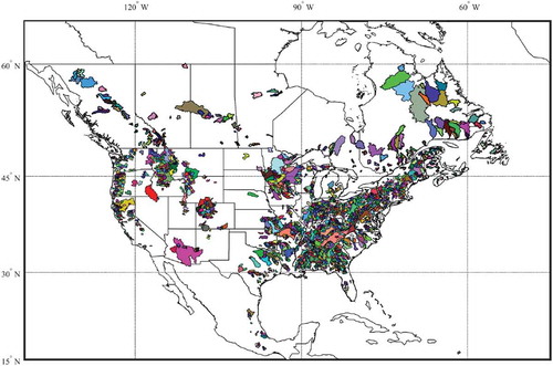
The data required for this study are the watershed area, daily precipitation, daily maximum and minimum temperatures and daily outflows. The reference period for the data is from 1 January 1950 to 31 December 2010. Hydrometeorological data come from the « Hydrometeorological Sandbox – École de technologie supérieure » (HYSETS) database (Arsenault et al. 2020). Some details of the watershed characteristics are listed in Table 1, such as average total annual precipitation (mm), average annual temperature (°C) and average annual streamflow (m³/s).

Table 1. Statistics from the 2080 watersheds in this study

	Area (km^2)	Precipitation (mm)	Temperature (°C)	Streamflow (m^3/s)	Longitude (°)	Latitude (°)
Minimum	303	270	−7.3	0.065	−132.2334	16.9867
25^th percentile	808	900	4.7	10.73	−105.8281	35.8094
Median	1480	1098	9.9	21.17	−87.8997	40.1265
75^th percentile	3773	1287	14.5	52.19	−81.8977	44.2949
Maximum	162 580	4336	22.7	1888	−54.1609	59.7833

3 Methodology

The methods used in this study at each step of the hydroclimatic modelling chain are presented in this section. Figure 2 presents a flowchart of the methodology. First, the hydrological models used to simulate low flows in each watershed are described along with the different PET formulas implemented in the modelling chain. Subsequently, the climate models and bias correction methods that were used are presented, followed by the PET and low-flow metrics that were analysed in current and future climates.

Figure 2. Flowchart of the project methodology

3.1 Potential evapotranspiration formulas

The simplest PET formulas are from the temperature-based and radiation-based categories, since they require less input data than in the case of the combinatorial formulas. The use of simple PET formulas requiring less data allows us to take into account a large number of watersheds, that are not all equipped with measuring instruments, to feed more complex formulas. In this study, 10 PET formulas are used: five from the temperature-based category and five from the radiation-based category. Temperature-based methods depend on temperature to calculate PET, while radiation-based methods use the principle of energy conservation to calculate PET (Xu and Singh 2002).

The inputs for the temperature-based formulas are maximum and minimum temperatures; sometimes Julian day and latitude are also required, to determine daylight duration. In addition to temperature, radiation-based formulas need information on extraterrestrial radiation. While temperature can be easily measured, the same cannot be said for the radiation reaching the Earth. Consequently, extraterrestrial radiation is calculated from the solar declination which depends on the latitude and Julian day. PET formulas used in this study are defined in Table 2. Formulas 1–5 are temperature based and formulas 6–10 are radiation based.

Table 2. Definition of the 10 PET formulas

Name (reference)	Formulas
1. Blaney and Criddle (BC) (Blaney and Criddle 1950)	$\mathrm{P}\mathrm{E}{\mathrm{T}}_{\mathrm{B}\mathrm{C}}=0.825\left(100\frac{\mathrm{D}\mathrm{L}}{365\ast 12}\right)\left(0.46{\mathrm{T}}_{\mathrm{m}}+8.13\right))$
2. Hamon (H) (Hamon 1960)	$\mathrm{P}\mathrm{E}{\mathrm{T}}_{\mathrm{H}}={\left(\frac{\mathrm{D}\mathrm{L}}{12}\right)}^{2}exp\left(\frac{{\mathrm{T}}_{\mathrm{m}}}{16}\right)$
3. Hydro-Quebec (HQ) (Fortin 2000)	$\mathrm{P}\mathrm{E}{\mathrm{T}}_{\mathrm{H}\mathrm{Q}}=0.029718\left({\mathrm{T}}_{max}-{\mathrm{T}}_{min}\right)exp\left(0.019\left(\frac{9}{5}\left({\mathrm{T}}_{max}+{\mathrm{T}}_{min}\right)\right.+\left.64\right)\right)$
4. Kharrufa (K) (Kharrufa 1985)	$\mathrm{P}\mathrm{E}{\mathrm{T}}_{\mathrm{K}}=0.34\left(100\frac{\mathrm{D}\mathrm{L}}{365\ast 12}\right){\mathrm{T}}_{\mathrm{m}}^{1.3}$
5. Mohyse (M) (Fortin and Turcotte 2006)	$\mathrm{P}\mathrm{E}{\mathrm{T}}_{\mathrm{M}}=\frac{4.088}{\pi }\omega \ast exp\left(\frac{17.3{\mathrm{T}}_{\mathrm{m}}}{238+{\mathrm{T}}_{\mathrm{m}}}\right)$
6. Baier and Robertson (BR) (Baier and Robertson 1965)	$\mathrm{P}\mathrm{E}{\mathrm{T}}_{\mathrm{B}\mathrm{R}}=0.157{\mathrm{T}}_{max}+0.158\left({\mathrm{T}}_{max}-{\mathrm{T}}_{min}\right)+0.019{\mathrm{R}}_{\mathrm{e}}-5.39$
7. Hargreaves and Samani (HS) (Hargreaves and Samani 1985)	$\mathrm{P}\mathrm{E}{\mathrm{T}}_{\mathrm{H}\mathrm{S}}=0.0023\frac{{\mathrm{R}}_{\mathrm{e}}}{\lambda \rho }\sqrt{\left({\mathrm{T}}_{max}-{\mathrm{T}}_{min}\right)}\left({\mathrm{T}}_{\mathrm{m}}+17.8\right)1000$
8. Jensen and Haise (JH) (Jensen and Haise 1963)	$\mathrm{P}\mathrm{E}{\mathrm{T}}_{\mathrm{J}\mathrm{H}}=1000\frac{{\mathrm{R}}_{\mathrm{e}}}{\lambda \rho }\frac{{\mathrm{T}}_{\mathrm{m}}}{40}$
9. McGuinness and Bordne (MB) (McGuinness and Bordne 1972)	$\mathrm{P}\mathrm{E}{\mathrm{T}}_{\mathrm{M}\mathrm{B}}=1000\frac{{\mathrm{R}}_{\mathrm{e}}}{\lambda \rho }\frac{{\mathrm{T}}_{\mathrm{m}}+5}{68}$
10. Oudin (O) (Oudin et al. 2005b)	$\mathrm{P}\mathrm{E}{\mathrm{T}}_{\mathrm{o}}=1000\frac{{\mathrm{R}}_{\mathrm{e}}}{\lambda \rho }\frac{{\mathrm{T}}_{\mathrm{m}}+5}{100}$

In these formulas, DL represents daylight duration (h/d), determined using the date and the latitude; T_m represents the daily mean air temperature (°C); ω represents the sunset angle (rad), determined from the date; T_max and T_min are the daily maximum and minimum air temperatures, respectively (°C); R_e represents the extraterrestrial radiation (MJ/m²d), determined from the date and latitude; and λ is the slope of the vapour pressure curve, determined using T_m and ρ, which is the water density (kg/L). PET values are in mm/d.

3.2 Hydrological modelling

To quantify the uncertainty of the hydroclimatic modelling chain components, it is necessary to use more than one hydrological model. Given the number of watersheds taken into account, data availability, computational time and data storage needed, lumped models were preferred to distributed models in this study. Lumped models have flexible structures, so they are able to adapt to different hydroclimatic conditions through empirical and parameterysed equations. Smith et al. (2012) demonstrated that lumped models can have generally similar performance to distributed models for the simulation of streamflows at the outlet of watersheds. The two hydrological models used in this study are GR4J (Génie Rural à 4 Paramètres – Journalier) and HMETS (Hydrological Model of the École de technologie supérieure). Both models give daily flows. While these models are both lumped and conceptual, they differ in their complexity and their internal structures, as described in the following sections. Both have been used in many hydrological and climate change impact studies (Brigode et al. 2013, Seiller and Anctil 2014, Troin et al. 2018, Zhao et al. 2020).

3.2.1 GR4J hydrological model

The GR4J hydrological model (Perrin et al. 2003) is a lumped model with four calibration parameters. Since GR4J does not take into account processes of snow accumulation and melt, CemaNeige (Valéry et al. 2014), a snow model with two calibration parameters, is used jointly with GR4J to simulate these snow processes. The internal structure of GR4J is based on two reservoirs: a production reservoir and a routing reservoir. Two unit hydrographs transform the water available for runoff into streamflow. Outflow from the first unit hydrograph (90% of the runoff water) first updates the level of the routing reservoir, which then contributes to streamflow through a relationship based on the reservoir level. Outflow from the second unit hydrograph (the remaining 10%) contributes directly to streamflow. CemaNeige’s inputs are the daily mean temperature and daily snowfall amount, and the output is the simulated snowmelt (snow water equivalent). GR4J’s inputs are the watershed area, total daily precipitation (including the simulated snowmelt from CemaNeige) and PET. The outputs of GR4J are the daily simulated streamflows.

3.2.2 HMETS hydrological model

The HMETS hydrological model (Martel et al. 2017) is also a lumped model, but it has 21 calibration parameters due to its more complex structure relative to GR4J. HMETS’ inputs are watershed area, daily temperatures (minimum and maximum), daily precipitation (solid and liquid, in water equivalent) and PET.

HMETS is based on two reservoirs: the vadose zone and the phreatic zone. The vadose zone provides water needed for hypodermic flow and groundwater recharge, depending on the reservoir water level, while a portion of the phreatic zone water allows groundwater flow. When a reservoir has reached its maximum capacity, water surplus is added to delayed runoff. The watershed streamflow is determined as a function of four horizontal components: (1) surface runoff, (2) delayed runoff, (3) hypodermic flow and (4) groundwater flow. Two unit hydrographs are used to transfer surface water and delayed runoff to streamflow.

3.3 Hydrological model calibration

Hydrological model calibration was performed automatically using the Shuffled Complex Evolution algorithm developed at the University of Arizona (SCEUA) (Duan et al. 1994). The maximum number of iterations is set to 10 000 in this study, following Arsenault et al. (2013). The calibration objective function is the Nash-Sutcliffe efficiency (NSE) (Nash and Sutcliffe 1970), described in Equation (1)(1) $NSE=1-\frac{{{\sum }_{t=1}^T\left(Q_{sim}^t-Q_{obs}^t\right)}^2}{{\sum }_{t=1}^T{\left(Q_{obs}^t-Q_M\right)}^2}$(1) . This objective function is frequently used in hydrology.

NSE measures the level of agreement between observed and simulated streamflows for the calibration period. The NSE value is between −∞ (bad performance) and 1 (perfect performance). An NSE value of 0 means the hydrological model performs as well as the mean observed flow would if it were used as a predictor.

(1) $NSE=1-\frac{{{\sum }_{t=1}^T\left(Q_{sim}^t-Q_{obs}^t\right)}^2}{{\sum }_{t=1}^T{\left(Q_{obs}^t-Q_M\right)}^2}$(1)

where t is the simulation time step (d), Q_sim,t represents the simulated streamflow for day t (m³/s), Q_obs,t represents the observed streamflow for day t (m³/s), Q_M is the mean of the observed streamflows (m³/s) and T is the total number of calibration time steps.

Calibration for each watershed is performed on the entire time period of available data. Arsenault et al. (2018) conclude that it is advantageous to calibrate on the longest possible period since in split-sample calibration and validation, data that could improve the calibration quality is omitted from the parameter set. In the context of climate change, model calibration quality impacts robustness and transferability in future conditions, justifying the need to preserve as much information as possible in the parameter set. A 2-year spin up period was used in the calibration process.

3.4 Climate change data

3.4.1 Climate models

Temperature and precipitation outputs from climate model projections are used to feed the hydrological models and PET formulas. The eight GCMs used in this study come from the Coupled Model Intercomparison Project – Phase 5 (CMIP5) ensemble (Taylor et al. 2012) and are presented in Table 3. The climate models were selected to cover the range of equilibrium climate sensitivity (ECS) of all the climate models available in the CMIP5 set (IPCC 2014). The ECS is the change in global and annual mean air temperature (°C) with double the atmospheric concentration of carbon dioxide of the pre-industrial period (IPCC 2014). Simulations with representative concentration pathways (RCP) 4.5 and 8.5 are taken into account in this study to analyse the impacts of greenhouse gas emissions scenario. The reference period is from 1 January 1971 to 31 December 2000, and the future periods are from 1 January 2041 to 31 December 2070 (horizon 2050) and 1 January 2071 to 31 December 2100 (horizon 2080).

Table 3. Description of the 8 GCMs from CMIP5

GCM	Year	Meteorological centre	Climate sensitivity	Spatial resolution (°)
CanESM2	2010	Canadian Centre for Climate Modelling and Analysis	3.7	2.8 × 2.8
CNRM-CM5	2010	Centre National de Recherches Météorologiques, Centre Européen de Recherche and Formation Avancées en Calcul Scientifique	3.3	1.4 × 1.4
CSIRO-Mk3.6.0	2009	Queensland Climate Change Centre of Excellence and Commonwealth Scientific and Industrial Research Organisation	4.1	1.8 × 1.8
GFDL-ESM2M	2011	NOAA Geophysical Fluid Dynamics Laboratory	2.4	2.5 × 2.0
GISS-E2-R	2011	NASA Goddard Institute for Space Studies USA	2.1	2.5 × 2.0
IPSL-CM5A-LR	2010	Institut Pierre Simon Laplace	4.1	3.75 × 1.8
MIROC5	2010	University of Tokyo, National Institute for Environmental Studies and Japan Agency for Marine-Earth Science and Technology	2.7	1.4 × 1.4
MIROC-ESM	2010	University of Tokyo, National Institute for Environmental Studies and Japan Agency for Marine-Earth Science and Technology	4.7	2.8 × 2.8

3.4.2 Post-processing

Post-processing is needed to correct the systematic biases of climate models over the reference period. During post-processing, there is an underlying hypothesis that the biases are stationary, which means that their statistical properties are temporally invariable. This allows the correction of future climate data using the same scale as corrections required in the reference period. Post-processing methods can be separated into two categories: change factor approaches and bias correction approaches (Chen et al. 2013). In this study, two post-processing methods are used, to represent the two categories. These are, respectively, daily scaling (DS) and daily bias correction (DBC).

3.4.2.1 Daily scaling

The DS method (Chen et al. 2013) is a quantile-based method, applied at a monthly time scale. Scaling factors are determined for each quantile of the distribution. The scaling factors represent the climate change signal projected by a climate model between the future and reference periods. DS is a change-factor method (delta change) because scaling factors are applied to observed meteorological data (Equations 2 and 3).

(2) $T_{fut,j}=T_{obs,j}+\left(T_{GCM,fut,Q}-T_{GCM,ref,Q}\right)$(2)

(3) $P_{fut,j}=P_{obs,j}\ast \left(P_{GCM,fut,Q}/P_{GCM,ref,Q}\right)$(3)

T_obs,j and P_obs,j represent observed temperature and precipitation on day j (°C and mm); T_fut,j and P_fut,j represent corrected temperature and precipitation on day j; T_GCM,fut,Q and P_GCM,fut,Q represent future temperature and precipitation from a climate model according to the month quantile and T_GCM,ref,Q and P_GCM,ref,Q represent temperature and precipitation for the reference period from the climate model according to the month quantile.

3.4.2.2 Daily bias correction

The DBC method (Chen et al. 2013) combines the daily translation method (DT) (Mpelasoka and Chiew 2009) and the local intensity scaling method (LOCI) (Schmidli et al. 2006). First, LOCI is applied to correct the occurrence of precipitation, to maintain the same frequency of rainy days in data from climate models as in the observed data. Next, DT is applied to correct temperature distributions and quantities of precipitation according to the quantiles. The DBC method is a bias correction method because scaling factors are applied to future data from climate models. The DT method is described in Equations (4)(4) $T_{fut,j}=T_{GCM,fut,j}+\left(T_{GCM,ref,Q}-T_{obs,Q}\right)$(4) and (5(5) $P_{fut,j}=P_{GCM,fut,j}\ast \left(P_{GCM,ref,Q}/P_{obs,Q}\right)$(5) ). The definitions of variables are the same as those for Equations (2)(2) $T_{fut,j}=T_{obs,j}+\left(T_{GCM,fut,Q}-T_{GCM,ref,Q}\right)$(2) and (3(3) $P_{fut,j}=P_{obs,j}\ast \left(P_{GCM,fut,Q}/P_{GCM,ref,Q}\right)$(3) ).

(4) $T_{fut,j}=T_{GCM,fut,j}+\left(T_{GCM,ref,Q}-T_{obs,Q}\right)$(4)

(5) $P_{fut,j}=P_{GCM,fut,j}\ast \left(P_{GCM,ref,Q}/P_{obs,Q}\right)$(5)

3.5 Metrics for PET and low flows

The combinatorial nature of this study generates a lot of data, because of the multiple (1) watersheds, (2) PET formulas, (3) hydrological models, (4) climate models, (5) post-processing methods and (6) greenhouse gas concentration scenarios – all of which are duplicated for the two future periods. To simplify the data analysis, this study focuses on five metrics.

3.5.1 PET metrics

To compare the different PET formulas, the mean annual PET (PET_m) and the maximum value of PET_m (PET_max), both in mm/d, are analysed.

3.5.2 Low-flow metrics

Characteristics of low-flow periods are different across North America because of the climate diversity. Nordic watersheds have low flows during winter when solid precipitation builds a snowpack. These winter periods are not investigated in this study since PET values are not significant when temperature is below freezing. Therefore, the chosen metrics are only computed when the daily minimum temperature is above 0°C. Furthermore, as the warm periods are not constant across the continent and subject to change in the future, the low-flow periods are therefore not identified according to fixed dates. For low-flow periods, the three metrics below are taken into account (Cloutier et al. 2007, CEHQ 2015). The definition of each metric is followed by a description of its usual function (Cloutier et al. 2007).

1. 7Q2 is the average low-flow value over 7 consecutive days with a 2-year return period (m³/s). 7Q2 is the low flow that must be maintained to protect aquatic life from conventional contaminants (suspended solids, phosphorus and biochemical oxygen demand) and fecal coliforms.

2. 7Q10 is the average low-flow value over 7 consecutive days with a 10-year return period (m³/s). 7Q10 is the low flow that must be maintained to protect aquatic life from toxic contaminants.

3. 30Q5 is the average low-flow value over 30 consecutive days with a 5-year return period (m³/s). 30Q5 is the low flow that must be maintained to protect drinking water supplies, and water consumption by aquatic organisms and by terrestrial wildlife.

The exceedance probability of low flows is based on the Log-Pearson type III law. The first 2 years of simulation are not considered for the calculation of low-flow metrics due to model spin-up time.

3.6 Uncertainty

To investigate the uncertainty in the PET formulas, a variance decomposition analysis (Déqué et al. 2007, Troin et al. 2018) was used. This statistical analysis evaluates the variance of each component of the hydroclimatic modelling chain and all possible interactions between them. The variance decomposition analysis was performed on all three low-flow metrics (7Q2, 7Q10 and 30Q5).

In this study, the hydroclimatic modelling chain contains five components: the PET formula (E), hydrological model (H), climate model (C), post-processing method (P) and RCP (R). Several component combinations are possible, with 10 possibilities for E, two for H, eight for C, two for P, and two for R, for a total possible number of 640 combinations. This analysis is made independently for each watershed. The variance of one component (for example, PET formula – E) is decomposed as in Equation (6)(6) ${\mathrm{V}}_{\mathrm{E}}=\mathrm{E}+\mathrm{E}\mathrm{H}+\mathrm{E}\mathrm{C}+\mathrm{E}\mathrm{P}+\mathrm{E}\mathrm{R}+\mathrm{E}\mathrm{H}\mathrm{C}+\mathrm{E}\mathrm{H}\mathrm{P}+\mathrm{E}\mathrm{H}\mathrm{R}+\mathrm{E}\mathrm{C}\mathrm{P}+\mathrm{E}\mathrm{C}\mathrm{R}+\mathrm{E}\mathrm{P}\mathrm{R}+\mathrm{E}\mathrm{H}\mathrm{C}\mathrm{P}+\mathrm{E}\mathrm{H}\mathrm{C}\mathrm{R}+\mathrm{E}\mathrm{C}\mathrm{P}\mathrm{R}+\mathrm{E}\mathrm{H}\mathrm{C}\mathrm{P}\mathrm{R}$(6) :

(6) ${\mathrm{V}}_{\mathrm{E}}=\mathrm{E}+\mathrm{E}\mathrm{H}+\mathrm{E}\mathrm{C}+\mathrm{E}\mathrm{P}+\mathrm{E}\mathrm{R}+\mathrm{E}\mathrm{H}\mathrm{C}+\mathrm{E}\mathrm{H}\mathrm{P}+\mathrm{E}\mathrm{H}\mathrm{R}+\mathrm{E}\mathrm{C}\mathrm{P}+\mathrm{E}\mathrm{C}\mathrm{R}+\mathrm{E}\mathrm{P}\mathrm{R}+\mathrm{E}\mathrm{H}\mathrm{C}\mathrm{P}+\mathrm{E}\mathrm{H}\mathrm{C}\mathrm{R}+\mathrm{E}\mathrm{C}\mathrm{P}\mathrm{R}+\mathrm{E}\mathrm{H}\mathrm{C}\mathrm{P}\mathrm{R}$(6)

4 Results

4.1 Hydrological model calibration

Both hydrological models were calibrated using each of the 10 PET formulas. The performance of each hydrological model calibration is presented in Fig. 3. For each hydrological model and PET formula combination, the boxplots show the NSE distribution for the 2080 watersheds. The two hydrological models have a similar median NSE performance of 0.77 for GR4J and 0.76 for HMETS.

Figure 3. Results of the hydrological model calibrations for the different potential evapotranspiration (PET) formulas

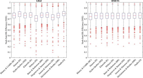
Although the median performance is similar, HMETS has a more constant performance across PET formulas. HMETS includes a calibration scaling parameter for PET. This parameter helps HMETS better adapt to different PET values, which explains the more constant performance of this model. With only four calibration parameters, GR4J does not have such a PET scaling parameter, so this model is more responsive to different PET values; instead, it uses a generic overall mass-balance term to simulate inter-watershed transfers that is constant in time. Also, GR4J boxplots in Fig. 3 have more extended outliers.

In Fig. 3, PET formulas are identified as BC (Blaney and Criddle), H (Hamon), HQ (Hydro-Quebec), K (Kharrufa), M (Mohyse), BR (Baier and Robertson), HS (Hargreaves and Samani), JH (Jensen and Haise), MB (McGuinness and Bordne) and O (Oudin).

Further analysis reveals differences among the three countries (not shown). For Canada, the medians are 0.81 for GR4J and 0.79 for HMETS. For the United States, the NSE median is 0.76 for both hydrological models. Finally, the NSE values for Mexican watersheds are systematically weaker for the two hydrological models. GR4J has more difficulty in adapting to the Mexican hydrology, with a median NSE of 0.33, whereas HMETS fares a little better, with a median NSE of 0.51. In Mexico, the transferability to future conditions is more questionable due to the lower calibration performance for the two hydrological models. The low reliability of hydrological databases explains most of the reduction in performance for the Mexican watersheds.

4.2 Analysis of parameter sensitivity to PET

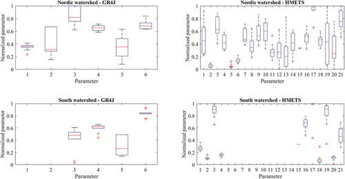
To evaluate the parameter sensitivity of the hydrological models to PET formulas, parameters of two watersheds were analysed: (1) a nordic watershed located in Quebec (Canada) and (2) a southern watershed located in Florida (United States). These watersheds were chosen as they represent two types of hydroclimatic conditions.

Figure 4 shows the boxplots of the normalysed parameter values for the HMETS and GR4J hydrological models. The normalization of the parameters was performed according to the maximum and minimum boundary values of each parameter. For GR4J, parameters 1 and 2 are those of the CemaNeige snow module, and parameters 3, 4, 5 and 6 are those of the main GR4J model. Of course, in the case of the southern watershed, the snow parameters are not included in the analysis since no snow-related processes are present in this watershed (parameters 1 and 2 for GR4J, and parameters 5–14 for HMETS). Figure 4 shows that varying the PET formula influences the values of the parameters. Overall, it can be seen that the parameter values show more variability in the case of the nordic watershed than in the case of the southern watershed. This can likely be explained by: (1) the higher number of parameters and hence the higher possible equifinality in the case of the nordic watershed; (2) the higher dispersion of mean annual PET cycles from the different PET formulas, again in the case of the nordic watershed.

Figure 4. Analysis of parameter sensitivity to potential evapotranspiration (PET) formulas

4.3 Impacts and trends in future climate

To evaluate the impacts of climate change on PET and low flows, the hydroclimatic modelling chain described above was applied to each watershed. This resulted in 640 values for each metric, covering the uncertainty of all components of the modelling chain.

The changes between reference period and future periods, for the different metrics, are expressed in terms of relative delta (Δ) (Equation 7(7) ${\mathrm{\Delta }}_i=\frac{V_{i,fut}-V_{i,ref}}{V_{i,ref}}$(7) ):

(7) ${\mathrm{\Delta }}_i=\frac{V_{i,fut}-V_{i,ref}}{V_{i,ref}}$(7)

V_i represents the value of metric i and the indices ref and fut represent, respectively, the reference period (1971–2000) and the future period (horizon 2050 or horizon 2080). The results shown in the following figures are the median relative delta from simulations using the two hydrological models, the eight climate models and the two post-processing methods.

Figure 5 shows the relative delta of the PET_m metric according to the different PET formulas for the 2071–2100 horizon and RCP 8.5. Every point in the figure represents the centroid of a watershed.

Figure 5. Relative delta between the reference period and the 2080 horizon for the PETm metric with RCP 8.5

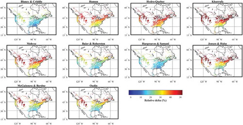
All PET formulas show an increase in ET across North America. This increase is consistent with the projected temperature increase. The intensity of the change is, however, spatially variable and highly dependent on the PET formula. The Kharrufa (K) and Hydro-Quebec (HQ) formulas give particularly large increases in PET. There does not seem to be a correlation between formulas of the same group (temperature-based or radiation-based), but some formulas can be grouped because they have the same behaviour, such as (1) Blaney & Criddle (BC) and Hargreaves & Samani (HS); (2) Hamon (H) and Mohyse (M); or (3) Jensen & Haise (JH), McGuinness & Bordne (MB) and Oudin (O).

For all of the PET formulas, the regions where PET increases are the highest are located in Canada and in the US Rocky Mountains, while the regions where PET increases are the lowest are located in Mexico and in the Southeastern United States. For the PET_max metric, the results (not shown) are similar, with the same trends.

Subsequently, Fig. 6 presents the results of relative delta between reference and future periods for the 7Q2 low-flow metric. The future conditions are the same as in Fig. 5, i.e. for the 2080 horizon and RCP 8.5.

Figure 6. Relative delta between the reference period and the 2080 horizon for the 7Q2 metric with RCP 8.5

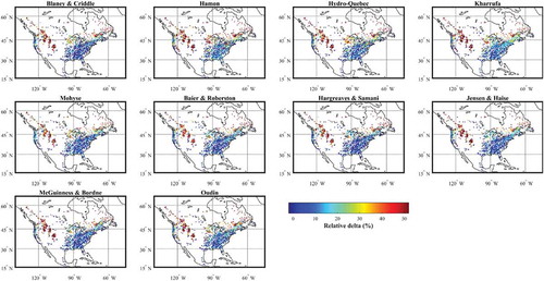
When looking at the results according to the broad regions identified from Fig. 5, there is more intra-region variability for the low-flow metrics than for the PET metrics. Contrary to the PET metrics, there is not much difference between the results obtained using the 10 PET formulas (Fig. 6). However, an important component of spatial variability remains, and regions where changes will be more important are again located in Canada and in the US Rocky Mountains, where the largest temperature increase is expected (Joyce et al. 2018, Martel 2019). The 7Q2 metric shows a general decreasing trend over the whole territory.

The variability between PET formulas is attenuated by hydrological models. For example, a formula that gets extreme PET metric values, such as Kharrufa (K), does not necessarily have more extreme values for low-flow metrics. This can likely be explained by the fact that there is not enough water availability to fulfil PET.

Figures 7 and Figures 8 show results for the 7Q10 and 30Q5 low-flow metrics, respectively, for the 2080 horizon and RCP 8.5. The trends of these two metrics are similar to those of the 7Q2 metric, but the intensity of changes is increased. Compared to current conditions, 30Q5 shows greater changes than 7Q2 and 7Q10 metrics.

Figure 7. Relative delta between the reference period and the 2080 horizon for the 7Q10 metric with RCP 8.5

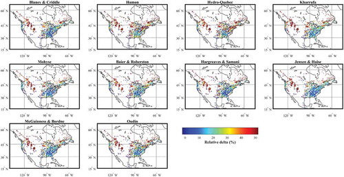
Figure 8. Relative delta between the reference period and the 2080 horizon for the 30Q5 metric with RCP 8.5

4.4 Uncertainty in hydroclimatic modelling

Variance decomposition analysis was carried out on the entire hydroclimatic modelling chain. This analysis was performed on the three low-flow metrics (in m³/s).

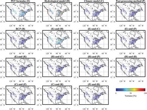
Figure 9 shows the results of the variance decomposition analysis for each low-flow metric, for the future period from 2071 to 2100 (2080 horizon). Boxplots in Fig. 9 show the variance distribution for the 2080 watersheds and for each component of the hydroclimatic modelling chain. The 2050 horizon results are similar and are not shown.

Figure 9. Variance decomposition analysis for the 7Q2, 7Q10 and 30Q5 low-flow metrics (2080 horizon)

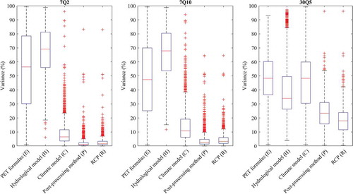
Results shown in Fig. 9 are the total variance of each component, so they represent the sum of the first-order variance of the component and the variances of each possible higher-order interaction with other components. This explains why the total variance of the five components sums to more than 100%.

For the 7Q2 metric, the hydrological model (H) has the largest variance, with a median of 69.1%, followed by the PET formula (E) with a median of 56.4%. Variances of climatic components are much smaller, with medians of 6.5% (C), 1.0% (P) and 1.7% (R). Results for the 7Q10 metric are similar, with medians of 67.8% (H), 47.3% (E), 10.7% (C), 2.5% (P) and 3.2% (R). An analysis of the 30Q5 metric shows different results. While the median variance of the PET formula remains similar (48.3%), the hydrological model (H) variance decreases to a median value of 34.0% and variances of climatic components increase, with medians of 48.8% (C), 23.3% (P) and 17.9% (R). In this case, the climate model is the component with the largest variance. Over a longer period, such as 30 d in this case, it is expected that the climate uncertainty will have a more important role.

An important point is the decomposition of total variances. Figure 10 shows the first- and second-order variances of the 7Q2 metric, for the future period from 2071 to 2100 (2080 horizon). For this metric, while the median total variances are 56.4% for E and 69.1% for H, the decomposition of these percentages reveals subtle yet interesting findings. The PET formula (E) median first-order variance is only 22.7%, and the hydrological model (H) median first-order variance is 32.5%, while the median variance of the second order interaction E–H is 27.6%. The rest of the variance comes from the other interactions with C, P and R. Therefore, the majority of the total PET variance is attributable to the interaction between the PET formula and the hydrological model.

Figure 10. First- and second-order interactions of the variance decomposition analysis of the 7Q2 low-flow metric (2080 horizon)

Table 4 shows the percentages of the variance decomposition of the various components for the three low-flow metrics. The interaction between E and H is significant in the total variance. For the 30Q5 metric, the results are lower because of the increased importance of climatic components in the total variance.

Table 4. Decomposition variance for PET formulas (E) only, hydrological model (H) only and interaction between E and H

	PET formulas (E)	Hydrological model (H)	Interaction between E and H
7Q2	22.7%	32.5%	27.6%
7Q10	17.9%	35.9%	21.6%
30Q5	16.4%	5.53%	9.53%

5 Discussion

5.1 Uncertainty from hydroclimatic chain components

In accordance with the results of Bae et al. (2011), hydrological components (PET formula and hydrological model) bring more uncertainty than do climatic components of the hydroclimatic modelling chain. Indeed, the structural uncertainty of hydrological modelling dominates the climate model uncertainty.

This study shows the advantage of taking into account several models and methods to quantify the uncertainty, which is consistent with the findings of Kay and Davies (2008), Minville et al. (2008), and Giuntoli et al. (2015). Although it is relevant to include several elements in each of the components of the hydroclimatic modelling chain, this must be done judiciously to avoid including elements which, by their poor performance or too-divergent behaviour, could generate false uncertainty.

5.2 The evaporation paradox

The results of this study show that increased ET is expected to modify the low-flow behaviour of rivers. However, recent studies have shown that ET levels have diminished even though the atmosphere is more energetic, is hotter and can theoretically contain more water. This has been termed the “Evaporation Paradox,” and was discovered by analysing lysimeter data over multiple regions of the world and verifying that pan evaporation has shown a decreasing trend while temperature trends have been increasing (Chattopadhyay and Hulme 1997, Quintana-Gomez 1998, Moonen et al. 2002, Asanuma and Kamimera 2004, Liu et al. 2004, Roderick and Farquhar 2004, 2005, Tebakari et al. 2005, Burn and Hesch 2007, Cong et al. 2009, Breña-Naranjo et al. 2017). Some proposed mechanisms to explain these results relate to increases in cloud cover and aerosols that reduce incoming radiation, smaller vapour pressure differentials due to more humid air, and decreasing wind speeds (Cong et al. 2009). In the case of this study, the PET methods used in hydrological modelling do not take into account any of these phenomena. It is therefore likely that some biases exist in the absolute changes estimated in low flows in the course of this study. However, it is also important to note that the hydrological models can compensate by having their model parameters adjusted to some extent during calibration to preserve streamflow.

5.3 Limitations

This study has some limitations that influence the results. In North America, the hydroclimatic diversity allows drawing broader conclusions and obtaining a better estimate of the spatial distribution of uncertainty. On the other hand, it can be tricky to implement a method on the entire study area and to generalyse from the conclusions with so many differences in hydrology and climate. The choice of a PET formula or a hydrological model can satisfy some conditions for the Canadian climate but may be less well-adapted for southern climates. Taking into account that the global climate is going to change, it is important to think about the transferability of the methods currently used. Working with a large number of watersheds, as is done in the present study, makes it possible to group them together and to distinguish the results by country or to identify spatial patterns according to future climate and PET changes.

The use of only two lumped and conceptual hydrological models is another limitation of this project. Using more hydrological models would increase the reliability of the uncertainty analysis of this component in the hydroclimatic modelling chain. Furthermore, the use of more physical and distributed models would provide the opportunity to better take into account evaporation and transpiration processes inside the hydrological model and their impacts on simulated streamflows. The choice to use simpler hydrological models mainly results from the large number of watersheds in this study as well as the increased amount of input data necessary to drive distributed and more physically based models.

Only one calibration method for hydrological modelling was used in this study. Since NSE gives high flows more weight than low flows during calibration (Krause et al. 2005, Gupta et al. 2009), this is probably not the best objective function in this case. It would be beneficial to explore other methods, such as calibrating only during low-flow periods, calibrating during summer time or using another objective function. On the other hand, NSE was used for all calibrations in this study, so they are equal and comparable even if they are not perfect for low-flow periods. The results of the variance decomposition and uncertainty attribution, described above, should therefore not be impacted by this choice. Consequently, the objective function plays a less critical role in the quantification of uncertainty of the other components in the hydroclimatic chain. Also, the results can be compared with other studies that use this objective function, such as that of Seiller and Anctil (2016).

6 Conclusion

This study investigated the effects of uncertainty in the components of the hydroclimatic modelling chain on future simulated PET and low flows. The studied area covers a wide domain, comprising 2080 watersheds spread over Canada, the United States and Mexico.

The hydroclimatic diversity present in the North American territory therefore allows to broader our conclusions and adds robustness to the results. The following components of the hydroclimatic modelling chain were taken into account: RCPs 4.5 and 8.5, eight global climate models, two post-processing methods, three lumped hydrological models, and 10 (temperature- or radiation-based) PET formulas; furthermore, the future horizons 2050 and 2080 were considered. All of the simulation results agree on a PET increase in all of the studied watersheds, with greater increases in Canada and in the US Rocky Mountains where higher increases in temperature are also expected. The intensity of the change is also highly dependent on the PET formula.

Three low-flow metrics, 7Q2, 7Q10 and 30Q5, were computed based on the future simulated flows and were also analysed. In accordance with simulated PET increases, the computed values of the metrics decrease under future conditions with respect to reference conditions. Spatial patterns remain in the results, but the variability induced by the PET formula is attenuated by hydrological models. All simulated changes are more pronounced under RCP 8.5 than under RCP 4.5, and in horizon 2080 than in horizon 2050.

A variance decomposition analysis was performed to better investigate the contributions of the different components of the hydroclimatic modelling chain to the uncertainty on low-flow metrics. The following main conclusions can be drawn from this analysis:

1. In the case of the 7Q2 and 7Q10 metrics, the most important contributions are from the hydrological models and PET formulas (highest total variance) with important interactions between the two components (second-order interaction variance higher than first-order variances);

2. In the case of the 30Q5 metric, most of the total variance comes from the climate models, but the contributions of the PET formulas and hydrological models remain important.

Structural uncertainty can therefore dominate climate model uncertainty, and this should be taken into consideration when carrying climate change impact studies on low flows. Using a single hydrological model–PET formula combination can lead to incomplete knowledge of possible future changes. Furthermore, the North American hydroclimatic diversity shows that the choice of methods is important depending on where a low-flow study is to be performed, and that this will be even more important in the future climate. It is recommended that water managers pay attention to such findings when identifying measures for adaptation to climate change. Further investigation should concentrate on improving ET modelling at the watershed scale to better represent the physics of the process, knowing that current practice is mainly limited to using PET formulas based on temperature as the main climate input.

Acknowledgements

The authors thank the École de technologie supérieure (ÉTS) and the Natural Sciences and Engineering Research Council of Canada (NSERC) for their financial support. We also thank Ouranos for providing climatic data used in this study. Furthermore, we thank the reviewers for their comments and suggestions for improving this paper.

Disclosure statement

No potential conflict of interest was reported by the authors.

References

- Anctil, F., Rousselle, J., and Lauzon, N., 2012. Hydrologie: cheminements de l’eau. 2e éd.. Québec, QC: Presses internationales Polytechnique.
- Arsenault, R., Brissette, F., and Martel, J.L., 2018. The hazards of split-sample validation in hydrological model calibration. Journal of Hydrology, 566, 346–362. doi:10.1016/j.jhydrol.2018.09.027
- Arsenault, R., et al., 2020. A comprehensive, multisource database for hydrometeorological modeling of 14,425 North American watersheds. Scientific Data, 7 (1), 1–12. doi:10.1038/s41597-020-00583-2
- Arsenault, R., et al., 2013. Comparison of stochastic optimization algorithms in hydrological model calibration. Journal of Hydrologic Engineering, 19 (7), 1374–1384. doi:10.1061/(ASCE)HE.1943-5584.0000938
- Asanuma, J. and Kamimera, H. (2004, March). Long-term trend of pan evaporation measurements in Japan and its relevance to the variability of the hydrological cycle. In Symposium on Water Resource and Its Variability in Asia in the 21st Century, Tsukuba, Japan.
- Bae, D.H., Jung, I.W., and Lettenmaier, D.P., 2011. Hydrologic uncertainties in climate change from IPCC AR4 GCM simulations of the Chungju Basin, Korea. Journal of Hydrology, 401 (1–2), 90–105. doi:10.1016/j.jhydrol.2011.02.012
- Baier, W. and Robertson, G.W., 1965. Estimation of latent evaporation from simple weather observations. Canadian Journal of Plant Science, 45 (3), 276–284. doi:10.1139/cjss-2017-0112
- Beven, K., 2001. On hypothesis testing in hydrology. Hydrological Processes, 15 (9), 1655–1657. doi:10.1002/hyp.436
- Blaney, H.F. and Criddle, W.D., 1950. Determining water requirements in irrigated areas from climatological and irrigation data. Washington, DC: US Departement of Agriculture, Soil Conservation Service.
- Breña-Naranjo, A., Laverde-Barajas, M.A., and Pedrozo-Acuña, A., 2017. Changes in pan evaporation in Mexico from 1960 to 2010. International Journal of Climatology, 37 (1), 204–213. doi:10.1002/joc.4698
- Brigode, P., Oudin, L., and Perrin, C., 2013. Hydrological model parameter instability: A source of additional uncertainty in estimating the hydrological impacts of climate change? Journal of Hydrology, 476, 410–425. doi:10.1016/j.jhydrol.2012.11.012
- Burn, D.H. and Hesch, N.M., 2007. Trends in evaporation for the Canadian Prairies. Journal of Hydrology, 336 (1–2), 61–73. doi:10.1016/j.jhydrol.2006.12.011
- CEHQ, (2015). Lignes directrices pour l’estimation des débits d’étiage sur le territoire québécois. Available from https://www.cehq.gouv.qc.ca/debit-etiage/methode/index.htm [Accessed 10 Feb 2019].
- Chattopadhyay, N. and Hulme, M., 1997. Evaporation and potential evapotranspiration in India under conditions of recent and future climate change. Agricultural and Forest Meteorology, 87 (1), 55–73. doi:10.1016/S0168-1923(97)00006-3
- Chen, J., et al., 2013. Finding appropriate bias correction methods in downscaling precipitation for hydrologic impact studies over North America. Water Resources Research, 49 (7), 4187–4205. doi:10.1002/wrcr.20331
- Cloutier, S., Gélineau, M., and Guay, I., 2007. Calcul et interprétation des objectifs environnementaux de rejet pour les contaminants du milieu aquatique. 2e éd. Québec, QC: Ministère du Développement durable, de l’Environnement et des Parcs.
- Cong, Z.T., Yang, D.W., and Ni, G.H., 2009. Does evaporation paradox exist in China? Hydrology and Earth System Sciences, 13 (3), 357–366. doi:10.5194/hess-13-357-2009
- Déqué, M., et al., 2007. An intercomparison of regional climate simulations for Europe: assessing uncertainties in model projections. Climatic Change, 81, 53–70. doi:10.1007/s10584-006-9228-x
- Duan, Q., Sorooshian, S., and Gupta, V.K., 1994. Optimal use of the SCE-UA global optimization method for calibrating watershed models. Journal of Hydrology, 158 (3–4), 265–284. doi:10.1016/0022-1694(94)90057-4
- Fortin, V., 2000. Le modèle météo-apport HSAMI: historique, théorie et application. Varennes, QC: Institut de recherche d’Hydro-Québec.
- Fortin, V. and Turcotte, R., 2006. Le modèle hydrologique MOHYSE.Montréal: Département des sciences de la terre et de l’atmosphère, Université du Québec à Montréal, Note de cours pour SCA7420.
- Giuntoli, I., et al., 2015. Future hydrological extremes: the uncertainty from multiple global climate and global hydrological models. Earth System Dynamics, 6, 267–285. doi:10.5194/esd-6-267-2015
- Gupta, H.V., et al., 2009. Decomposition of the mean squared error and NSE performance criteria: implications for improving hydrological modelling. Journal of Hydrology, 377 (1–2), 80–91. doi:10.1016/j.jhydrol.2009.08.003
- Hamon, W.R., (1960). Estimating potential evapotranspiration. (Thèse de doctorat. Massachusetts Institute of Technology, États-Unis).
- Hargreaves, G.H. and Samani, Z.A., 1985. Reference crop evapotranspiration from temperature. Applied Engineering in Agriculture, 1 (2), 96–99. doi:10.13031/2013.26773
- Intergovernmental Panel on Climate Change (IPCC), 2014. Climate change 2013: the physical science basis. Contribution of working group I to the fifth assessment report of the intergovernmental panel on climate change. Cambridge, United Kingdom: Cambridge University Press.
- Jensen, M.E. and Haise, H.R., 1963. Estimating evapotranspiration from solar radiation. Proceedings of the American Society of Civil Engineers. Journal of the Irrigation and Drainage Division, 89, 15–41.
- Joyce, L.A., et al., 2018. Historical and projected climate in the Northern Rockies region. Advances in Global Change Research, 63, 17–23. doi:10.1007/978-3-319-56928-4_2
- Kay, A.L. and Davies, H.N., 2008. Calculating potential evaporation from climate model data: A source of uncertainty for hydrological climate change impacts. Journal of Hydrology, 358 (3–4), 221–239. doi:10.1016/j.jhydrol.2008.06.005
- Kharrufa, N.S., 1985. Simplified equation for evapotranspiration in arid regions. Beiträge Zur Hydrologie, 5 (1), 39–47.
- Kingston, D.G., et al., 2009. Uncertainty in the estimation of potential evapotranspiration under climate change. Geophysical Research Letters, 36 (20). doi:10.1029/2009GL040267
- Kirchner, J.W., 2006. Getting the right answers for the right reasons: linking measurements, analyses, and models to advance the science of hydrology. Water Resources Research, 42 (3). doi:10.1029/2005WR004362
- Krause, P., Boyle, D.P., and Bäse, F., 2005. Comparison of different efficiency criteria for hydrological model assessment. Advances in Geosciences, 5, 89–97. doi:10.5194/adgeo-5-89-2005
- Liu, B., et al., 2004. A spatial analysis of pan evaporation trends in China, 1955–2000. Journal of Geophysical Research: Atmospheres, 109 (D15). doi:10.1029/2004JD004511
- Martel, J.L., 2019. École de technologie supérieure: Évaluation de l’influence de la variabilité naturelle du climat et des changements climatiques anthropiques sur les extrêmes hydrométéorologiques. (Doctoral dissertation.
- Martel, J.L., et al., 2017. HMETS-A simple and efficient hydrology model for teaching hydrological modelling, flow forecasting and climate change impacts. International Journal of Engineering Education, 33 (4), 1307–1316.
- McGuinness, J.L. and Bordne, E.F., 1972. A comparison of lysimeter-derived potential evapotranspiration with computed values (No. 1452). Washington, DC: US Dept. of Agriculture.
- McMahon, T.A., Finlayson, B.L., and Peel, M.C., 2016. Historical developments of models for estimating evaporation using standard meteorological data. Wiley Interdisciplinary Reviews: Water, 3 (6), 788–818. doi:10.1002/wat2.1172
- Minville, M., Brissette, F., and Leconte, R., 2008. Uncertainty of the impact of climate change on the hydrology of a nordic watershed. Journal of Hydrology, 358 (1–2), 70–83. doi:10.1016/j.jhydrol.2008.05.033
- Minville, M., et al., 2014. Improving process representation in conceptual hydrological model calibration using climate simulations. Water Resources Research, 50 (6), 5044–5073. doi:10.1002/2013WR013857
- Moonen, A.C., et al., 2002. Climate change in Italy indicated by agrometeorological indices over 122 years. Agricultural and Forest Meteorology, 111 (1), 13–27. doi:10.1016/S0168-1923(02)00012-6
- Mpelasoka, F.S. and Chiew, F.H., 2009. Influence of rainfall scenario construction methods on runoff projections. Journal of Hydrometeorology, 10 (5), 1168–1183. doi:10.1175/2009JHM1045.1
- Nash, J.E. and Sutcliffe, J.V., 1970. River flow forecasting through conceptual models part I—A discussion of principles. Journal of Hydrology, 10 (3), 282–290. doi:10.1016/0022-1694(70)90255-6
- Oudin, L. (2004). Recherche d’un modèle d’évapotranspiration potentielle pertinent comme entrée d’un modèle pluie-débit global. (Thèse de doctorat. Paris: École Nationale du Génie Rural, des Eaux et des Forêts (ENGREF)).
- Oudin, L., et al., 2005a. Which potential evapotranspiration input for a lumped rainfall–runoff model?: part 2—Towards a simple and efficient potential evapotranspiration model for rainfall–runoff modelling. Journal of Hydrology, 303 (1–4), 290–306. doi:10.1016/j.jhydrol.2004.08.026
- Oudin, L., Michel, C., and Anctil, F., 2005b. Which potential evapotranspiration input for a lumped rainfall-runoff model?: part 1—Can rainfall-runoff models effectively handle detailed potential evapotranspiration inputs? Journal of Hydrology, 303 (1–4), 275–289. doi:10.1016/j.jhydrol.2004.08.025
- Perrin, C., Michel, C., and Andréassian, V., 2003. Improvement of a parsimonious model for streamflow simulation. Journal of Hydrology, 279 (1–4), 275–289. doi:10.1016/S0022-1694(03)00225-7
- Quintana-Gomez, R.A., 1998. Changes in evaporation patterns detected in northernmost South America. In: Proc 7th int. meeting on statistical climatology. Whistler, BC, Canada: Institute of Mathematical Statistics, 97.
- Ricard, S. and Anctil, F., 2019. Forcing the Penman-Montheith formulation with humidity, radiation, and wind speed taken from reanalyses, for hydrologic modeling. Water, 11 (6), 1214. doi:10.3390/w11061214
- Roderick, M.L. and Farquhar, G.D., 2004. Changes in Australian pan evaporation from 1970 to 2002. International Journal of Climatology: A Journal of the Royal Meteorological Society, 24 (9), 1077–1090. doi:10.1002/joc.1061
- Roderick, M.L. and Farquhar, G.D., 2005. Changes in New Zealand pan evaporation since the 1970s. International Journal of Climatology: A Journal of the Royal Meteorological Society, 25 (15), 2031–2039. doi:10.1002/joc.1262
- Schmidli, J., Frei, C., and Vidale, P.L., 2006. Downscaling from GCM precipitation: a benchmark for dynamical and statistical downscaling methods. International Journal of Climatology: A Journal of the Royal Meteorological Society, 26 (5), 679–689. doi:10.1002/joc.1287
- Seiller, G. and Anctil, F., 2014. Climate change impacts on the hydrologic regime of a Canadian river: comparing uncertainties arising from climate natural variability and lumped hydrological model structures. Hydrology and Earth System Sciences, 18 (6), 2033–2047. doi:10.5194/hess-18-2033-2014
- Seiller, G. and Anctil, F., 2016. How do potential evapotranspiration formulas influence hydrological projections? Hydrological Sciences Journal, 61 (12), 2249–2266. doi:10.1080/02626667.2015.1100302
- Smith, M.B., et al., 2012. Results of the DMIP 2 Oklahoma experiments. Journal of Hydrology, 418, 17–48. doi:10.1016/j.jhydrol.2011.08.056
- Taylor, K.E., Stouffer, R.J., and Meehl, G.A., 2012. An overview of CMIP5 and the experiment design. Bulletin of the American Meteorological Society, 93 (4), 485–498. doi:10.1175/BAMS-D-11-00094.1
- Tebakari, T., Yoshitani, J., and Suvanpimol, C., 2005. Time-space trend analysis in pan evaporation over kingdom of Thailand. Journal of Hydrologic Engineering, 10 (3), 205–215. doi:10.1061/(ASCE)1084-0699(2005)10:3(205)
- Troin, M., et al., 2018. Uncertainty of hydrological model components in climate change studies over two Nordic Quebec Catchments. Journal of Hydrometeorology, 19 (1), 27–46. doi:10.1175/JHM-D-17-0002.1
- Valéry, A., Andréassian, V., and Perrin, C., 2014. ‘As simple as possible but not simpler’: what is useful in a temperature-based snow-accounting routine? Part 2–Sensitivity analysis of the Cemaneige snow accounting routine on 380 catchments. Journal of Hydrology, 517, 1176–1187. doi:10.1016/j.jhydrol.2014.04.058
- Xu, C.Y. and Singh, V.P., 2002. Cross comparison of empirical equations for calculating potential evapotranspiration with data from Switzerland. Water Resources Management, 16 (3), 197–219. doi:10.1023/A:1020282515975
- Zhao, C., et al., 2020. Frequency change of future extreme summer meteorological and hydrological droughts over North America. Journal of Hydrology, 584, 124316. doi:10.1016/j.jhydrol.2019.124316