Streamflow estimation using satellite-retrieved water fluxes and machine learning technique over monsoon-dominated catchments of India

ABSTRACT

In this study, advanced scatterometer (ASCAT) soil moisture data is employed to compute the basin water index (BWI) over six river basins of India for 10 years (2007–2016). The BWI time series is assessed for the development of its relationship with observed streamflow. Further, a popular ensemble learning technique, random forest, is employed to compute the 10-d streamflow using the BWI time series. Moreover, the results are compared with the classical rainfall–runoff model forced with satellite-based precipitation and evapotranspiration, BWI–rainfall–runoff model, and Global Flood Awareness System (GloFAS). The performance of the model is evaluated in terms of multiple efficiency measures, viz. Nash-Sutcliffe efficiency (NSE), correlation coefficient (R) and root mean square error (RMSE). The results reveal the BWI–rainfall–runoff model is the most accurate model for prediction of discharge. The performance of the BWI–rainfall–runoff model is very good over four of six catchments and good to satisfactory over the remaining two catchments.

KEYWORDS:

• scatterometer
• soil moisture
• BWI
• machine learning
• random forest
• Indian river basins

Editor A. Fiori Associate Editor D. Rivera

1 Introduction

Soil moisture is a key factor that drives the hydrological cycle. Measuring soil moisture reliably at a global scale can be used to solve various problems in the fields of hydrology, agriculture, and meteorology, e.g. irrigation scheduling, water management, runoff prediction, etc. (Houser et al. 1998, Wagner et al. 1999, 2007, Brocca et al. 2010, 2016, 2017). To study the behavioural pattern of runoff, knowledge of soil moisture is crucial, as the partitioning of rainfall to runoff and infiltration is controlled by soil moisture amongst other important factors (such as soil hydraulic properties, land cover, topography and climatic factors). Therefore, soil moisture has a significant influence on the runoff process of the river basins (Aubert et al. 2003, Brocca et al. 2017). From a hydrological point of view, it is important to measure the soil moisture both spatially and temporally, which can be an effective tool in predicting the runoff pattern and also to improve and validate hydrological representations. For spatial coverage, many point measurements of soil moisture are required, which is very costly, and only a few measurement programmes have gathered a considerable amount of soil moisture data (Georgakakos and Baumer 1996).

Remote sensing is recognized as a useful tool to monitor soil moisture at different spatial and temporal scales (Schmugge 1983, Engman and Chauhan 1995, Ceballos et al. 2005). Satellite data can be used to determine the soil moisture content from microwave sensors, and both passive and active sensors are found to be effective (Jackson 1993, Engman and Chauhan 1995, Njoku and Entekhabi 1996). The advanced scatterometer (ASCAT) provides the backscatter coefficient at a high temporal resolution (1–2 d globally), and has been used in various studies to estimate surface soil moisture. Several prior studies (Wagner et al. 1999, 2003, 2007, Scipal et al. 2005, Naeimi et al. 2009, Meier et al. 2011) reported the potential for satellite-measured soil moisture data to be applied over large areas. Ceballos et al. (2005) evaluated the European Remote Sensing (ERS)-scatterometer-retrieved soil moisture using ground-based measurements taken globally with an accuracy of 2.2 vol% for semi-arid parts of the Duero Basin (Spain). Paulik et al. (2014) validated the ASCAT soil water index using the in situ soil moisture from 664 stations and found it to have reasonable accuracy.

Before developing any hydrological modelling scheme, it is important to understand the available information. There are various models available that use land-use maps, soil maps, weather data (precipitation, solar radiation, relative humidity, wind speed), etc. as input variables (Dhami et al. 2018). The incorporation of these relevant input variables improves the understanding of the modelling processes. For hydrological problems such as runoff prediction, flood forecasting, and drought monitoring, the use of in situ soil moisture observations may not be feasible. Therefore, the soil moisture retrieved from satellite data can be employed in hydrological modelling, particularly in the assimilation scheme of land-surface hydrologic models (Alvarez-Garreton et al. 2014, Rafieeinasab et al. 2014, Baguis and Roulin 2017, Loizu et al. 2018, Patil and Ramsankaran 2018). Studies carried out by Scipal et al. (2005) and Meier et al. (2011) revealed that finding a relation between discharge and soil moisture can enhance the modelling approach and help in predicting runoff at the basin scale.

Rainfall–runoff modelling is the core of hydrologic modelling, which has improved significantly over time due to the incorporation of more input parameters. Evapotranspiration (ET) is a key process in the hydrological cycle that plays a vital role in governing streamflow. Therefore, most studies recommend using precipitation minus ET as they represent the actual water available that can generate runoff. However, the in situ data for ET are rarely available, particularly in developing and underdeveloped countries. With the advent of satellite sensors, it is possible to obtain ET products at finer spatiotemporal resolutions. Nevertheless, the importance of soil moisture is definite, especially for modelling discharge at large scales. In this regard, the application of a hydrological model forced with satellite-based rainfall, ET and soil moisture can be useful.

Although physics-based rainfall–runoff models are enormously useful in understanding the governing processes, they require several input parameters (Himanshu et al. 2018). Most of these are challenging to obtain at the desired quality and thus, the calibration of these models requires a considerable amount of time and human effort (Gupta et al. 1998, Kokkonen and Jakeman 2001, Kavetski et al. 2003, Silberstein 2006, Pandey et al. 2008, Liu et al. 2009, Suryavanshi et al. 2017, Himanshu et al. 2018). Having the advantage of overcoming these constraints, data-driven hydrological models have risen in popularity for the estimation of river discharge. The commonly used data-driven techniques are artificial neural networks (ANNs), multiple linear regression (MLR), support vector machines (SVMs) and regression trees (Londhe and Charhate 2010, Elshorbagy et al. 2010a, 2010b).

Halff et al. (1993) designed an ANN model to predict the runoff hydrograph considering rainfall hyetographs as an input parameter, which opened up paths for the subsequent applications of ANN for rainfall–runoff modelling (Hsu et al. 1995, Sudheer et al. 2002, Agarwal and Singh 2004, Antar et al. 2006). Chen et al. (2008) applied SVM for the estimation of monthly discharge of the Yangtze River of China and revealed the model to possess high accuracy with the observed flows. Wu et al. (2009) utilized crisp distributed support vector regression (CDSVR), autoregressive moving average, K-nearest neighbour (KNN) and ANN for monthly streamflow prediction. Elshorbagy et al. (2010b) implemented ANN, KNN, MLR, SVM, M5 model trees, genetic programming and evolutionary polynomial regression for runoff prediction utilizing rainfall, ET and soil moisture as inputs. Similarly, Nayak et al. (2013) demonstrated the potential of ANN and wavelet neural network (WNN) for streamflow estimation utilizing rainfall and ET as inputs for the Malaprabha basin in India. Some recent applications of ensemble learning techniques (e.g. random forest) are also available in the hydrology literature (Yaseen et al. 2016, Chiang et al. 2018, Prieto et al. 2019). These data-driven techniques, as compared to physics-based hydrological models, require less parameterization and less development time, and have proven to be capable of accurately estimating stream flows (Wu et al. 2009, Kisi et al. 2012).

The newly developed datasets with high temporal resolution (such as scatterometer-retrieved soil moisture), machine learning-based ensemble techniques, and availability of high computational facilities may be useful for hydrological modelling. However, the potential to use these soil moisture datasets and algorithms for the estimation of streamflow has not been investigated over the Indian river basins. Further, the use of satellite-based soil moisture to improve the performance of the classical rainfall–runoff model (especially forced with satellite-based ET and rainfall) is often not explored well. Nowadays, the advances in remote sensing and numerical weather prediction have led to the development of global runoff products, e.g. the Global Flood Awareness System (GloFAS), which is an operational system for ensemble streamflow prediction over the large rivers worldwide (Revilla-Romero et al. 2015, Dottori et al. 2016, Hirpa et al. 2018, Harrigan et al. 2020). A comparison of the model results with GloFAS for accuracy in discharge estimation can be useful to gain valuable insights regarding the reliability of global runoff products.

Looking into the aforementioned issues, the objectives of this study are: (1) to evaluate the applicability of a machine learning-based framework for streamflow estimation solely based on advanced scatterometer data; (2) to compare the results with a machine learning-based hydrological model forced with satellite-based rainfall and ET; (3) to investigate the improvement in discharge prediction of the hydrological model by incorporating satellite soil moisture along with rainfall and ET; and (4) to compare the results with those obtained using GloFAS. Such a comprehensive assessment on developing simplified approaches for estimating river discharge from satellite observations could be highly beneficial; however, no previous study is found to have addressed the same questions. Further, this study will be instrumental in identifying the major contributor to the discharge among the inputs (rainfall, soil moisture, evapotranspiration).

2 Study area

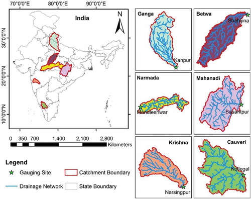
In this study, six catchments of large and medium river basins of India (Ganga, Betwa, Narmada, Mahanadi, Krishna and Cauvery) are considered to evaluate the modelling approaches. Information about each gauging site and their spatial locations are presented in Table 1 and Fig. 1, respectively. The size of the selected catchments varies from 21 082 to 86 437 km². Detailed information about each basin is provided below.

Table 1. Information on the river basins and gauging sites used in the study and their data availability

River basin	Gauging site	Latitude (°N)	Longitude (°E)	Catchment area (km^2)	Data availability
Ganga	Kanpur	26.48	80.40	86 437	June 2009–May 2016
Betwa	Shjahijina	25.88	80.23	43 936	January 2007–May 2014
Narmada	Mandleshwar	22.17	75.66	72 809	January 2007–December 2016
Mahanadi	Basantpur	21.72	82.79	68 450	January 2007–December 2015
Krishna	Narasingpur	17.97	75.14	22 856	January 2007–December 2015
Cauvery	Kollegal	12.19	77.10	21 082	January 2007–December 2016

Figure 1. Study domain showing the catchments of different river basins and gauging sites

2.1 Ganga basin

The Ganga sub-basin up to Kanpur gauging site is considered in this study. It falls within the upper and middle Ganga basin area and lies between 26.45 and 31.46°N latitude and between 77.63 and 80.57°E longitude. The Ganga River is one of the principal rivers of India and flows through the alluvial Gangetic Plains of northern India. The total area of the sub-basin is about 86 437 km². The topography of the basin varies from the hilly mountains of the Himalayas to alluvial plains, and the elevation ranges from 88 to 7512 m a.s.l. The soil type is classified into loamy, sandy, clayey and loamy-skeletal soils, rock outcrops and glaciers. More than half of the study area has a loamy soil type. The catchment is covered with agricultural lands, forests, shrubs and snow cover (India-WRIS 2014). The basin falls within the sub-tropical climate zone and thus, experiences hot and humid summers and cold winters. The rainfall over the basin predominantly occurs in the monsoon season (June–September).

2.2 Betwa basin

Betwa River basin is positioned in the central part of India and covers five districts of southern Uttar Pradesh and 10 districts of Madhya Pradesh. It extends from 22.86 to 26.05°N and from 77.09 to 80.23°E. The total area of the basin is approximately 43 930 km², of which 69% falls within Madhya Pradesh and 31% falls within Uttar Pradesh. The Shahijina station is located at the outlet of the basin. The basin area has varying complex patterns of vegetation and topography, i.e. from flat wheat-growing farmlands to steep hilly forests, with agriculture as the major land use. The climate of the Betwa basin is moderate, mostly dry except for the monsoon season (India-WRIS 2014). The average annual rainfall over the basin is 1138 mm and almost 90% of it occurs during June to mid-October. The daily mean temperature ranges from less than 10°C in the winter season to above 40°C in the summer seasons.

2.3 Narmada basin

The Narmada River basin up to the Mandleshwar gauging site covers a catchment area of 72 809 km². It falls within the Madhya Pradesh state of central India and extends from 21.39 to 23.78°N and from 75.36 to 81.77°E. The topography of the basin varies from an upper hilly region to alluvial plains, and the elevation ranges from 131 to 1317 m a.s.l. The Narmada basin mainly consists of black soils, and the plains are broad, fertile and well suited for cultivation. The climatic condition of the basin is generally tropical and wet, although in some parts of the basin, extreme heat and cold are experienced often (India-WRIS 2014). The annual rainfall in the upper part of the basin is about 1400 mm. The temperature during summer is very high (normally above 40°C during May), whereas it varies from 8 to 20°C during the winter season.

2.4 Mahanadi basin

The Mahanadi basin up to the Basantpur gauging site has a catchment area of 68 450 km². A major portion of the catchment lies in Chhattisgarh state and is situated between 19.93 and 23.56°N and between 80.43 and 83.60°E. The climatic region is tropical with a hot and wet monsoon. The average annual precipitation is 1572 mm, of which 70% occurs during the southwest monsoon season (June–October). The climate is hot and very humid during summer, whereas it is cold in the winter season. This basin is very susceptible to floods and is affected by disastrous floods almost annually (India-WRIS 2014).

2.5 Krishna basin

The gauging station considered in this river basin is Narsingpur, covering a catchment area of 22 856 km². It is located in the Maharashtra state of India and lies between 17.93 and 19.41°N and between 73.34 and 75.31°E. It is the second-largest river basin after Godavari basin in Peninsular India. The catchment mainly consists of black and red soils, with undulating topography and elevation ranging from 447 to 1471 m a.s.l. It causes heavy soil erosion during the monsoon floods. The average annual rainfall of the basin is 784 mm (India-WRIS 2014). While the climate is hot and humid during the summer, it is mild during the winter season. The mean daily temperature varies from 35 to 40°C (March–June).

2.6 Cauvery basin

The gauging station considered in this river basin is Kolllegal, with a catchment area of about 21 082 km², located between 11.47 and 13.39°N and between 75.49 and 77.21°E. A major part of the catchment lies within the Karnataka state. The climate of the river basin is tropical sub-humid, receiving an average annual rainfall of approximately 1100 mm. The major soil types present in the basin are black, red, laterites and mixed. The recorded maximum and minimum temperatures over the basin are 44°C and 18°C, respectively (India-WRIS 2014).

3 Data and methodology

3.1 Datasets used

Relevant information on all the datasets utilized in the present study is provided in Table 2. The study area catchments were delineated using the Shuttle Radar Topography Mission digital elevation model (SRTM DEM) at 90 m resolution. The satellite-based datasets that are utilized in the study are surface soil moisture, rainfall and evapotranspiration products. The other datasets that are utilized are ground-based maximum and minimum temperature, wind speed, and river discharge from GloFAS (http://www.globalfloods.eu/). The reference dataset is the river discharge data, which was obtained from the Water Resources Information System (www.india-wris.nrsc.gov.in), Central Water Commission (CWC), India.

Table 2. Summary of the datasets used in the study

Dataset	Source	Spatial resolution	URL/reference
Soil moisture	H-SAF (H-113)	12.5 km	http://hsaf.meteoam.it/soil-moisture.php
Rainfall	IMERG V06	0.1° × 0.1°	https://gpm.nasa.gov/data-access/downloads/gpm
Evapotranspiration (ET)	MODIS (MOD16A2GFv006)	500 m	https://lpdaac.usgs.gov/products/mod16a2gfv006/
Temperature (maximum and minimum)	IMD gridded	1° × 1°	Srivastava et al. (2009);http://www.imdpune.gov.in/Clim_Pred_LRF_New/Grided_Data_Download.html
Wind speed	NCEP–CFSR	0.25° × 0.25°	http://globalweather.tamu.edu/
GloFAS discharge	ECMWF GloFAS v2.1	0.1° × 0.1°	Harrigan et al. (2020)https://cds.climate.copernicus.eu/cdsapp#!/dataset/cems-glofas-historical?tab=overview
Observed discharge	CWC gauge	-	http://india-wris.nrsc.gov.in/
Topography	SRTM DEM	90 m	http://srtm.csi.cgiar.org/srtmdata/

3.1.1 Surface soil moisture or soil wetness index

The surface soil moisture product (H-113) was developed using the backscattering coefficients measured by the ASCAT instrument onboard the MetOp-A, B under the H-SAF (Satellite Application Facility on Support to Operational Hydrology) project of the European Organisation for the Exploitation of Meteorological Satellites (EUMETSAT). It is available at a grid spacing of 12.5 km with an irregular temporal sampling rate of every 1–2 d (depending on the latitude).

For retrieval of surface soil moisture from ASCAT’s Backscatter data, an algorithm developed by the Vienna University of Technology, or TU Wein (Wagner et al. 1999), was utilized for the development of surface soil moisture under the H-SAF project. From a mathematical point of view, the change detection algorithm developed by TU Wein is found to be easy and simple to use compared to other physical, empirical and semi-empirical modelling approaches. Equation (1)(1) $\mathrm{S}{\mathrm{M}}_t=\frac{{\sigma }^{\circ }\left(t,{\theta }_{\mathrm{r}\mathrm{e}\mathrm{f}}\right)-\sigma { }_{\mathrm{d}\mathrm{r}\mathrm{y}}^{\circ }\left({\theta }_{\mathrm{r}\mathrm{e}\mathrm{f}}\right)}{\sigma { }_{\mathrm{w}\mathrm{e}\mathrm{t}}^{\circ }\left({\theta }_{\mathrm{r}\mathrm{e}\mathrm{f}}\right)-\sigma { }_{\mathrm{d}\mathrm{r}\mathrm{y}}^{\circ }\left({\theta }_{\mathrm{r}\mathrm{e}\mathrm{f}}\right)}$(1) shows the methodology used to retrieve the surface soil moisture SM_t, considering the lowest and highest backscatter values:

(1) $\mathrm{S}{\mathrm{M}}_t=\frac{{\sigma }^{\circ }\left(t,{\theta }_{\mathrm{r}\mathrm{e}\mathrm{f}}\right)-\sigma { }_{\mathrm{d}\mathrm{r}\mathrm{y}}^{\circ }\left({\theta }_{\mathrm{r}\mathrm{e}\mathrm{f}}\right)}{\sigma { }_{\mathrm{w}\mathrm{e}\mathrm{t}}^{\circ }\left({\theta }_{\mathrm{r}\mathrm{e}\mathrm{f}}\right)-\sigma { }_{\mathrm{d}\mathrm{r}\mathrm{y}}^{\circ }\left({\theta }_{\mathrm{r}\mathrm{e}\mathrm{f}}\right)}$(1)

where SM_t is a relative measure of the soil moisture content in the first few centimetres of the soil, ranging between 0 (completely dry condition) and 1 (saturation condition) as it is expressed in terms of relative soil moisture (or degree of saturation). ${\sigma }^{\circ }\left(t,{\theta }_{\mathrm{r}\mathrm{e}\mathrm{f}}\right)$is the backscatter coefficient (in dB) at time t and reference angle ${\theta }_{\mathrm{r}\mathrm{e}\mathrm{f}}$, $\sigma { }_{\mathrm{d}\mathrm{r}\mathrm{y}}^{\circ }\left({\theta }_{\mathrm{r}\mathrm{e}\mathrm{f}}\right)$ is the backscatter coefficient in dry conditions (long-term lowest value of backscatter), $\sigma { }_{\mathrm{w}\mathrm{e}\mathrm{t}}^{\circ }\left({\theta }_{\mathrm{r}\mathrm{e}\mathrm{f}}\right)$is the backscatter coefficient in wet conditions (long-term highest value of backscatter). All the backscattering (σ°) values are measured at a reference incidence angle of 40°.

3.1.2 Rainfall

Daily satellite-based precipitation data were prepared from the Integrated Multi-satellitE Retrievals for Global Precipitation Measurement (IMERG) V06 (Final Run) half-hourly product (Huffman et al. 2019). The data has a spatial resolution of 0.1° and a temporal resolution of 30 min, and is available at a latency of 3.5 months from real time. This product is prepared from the calibrated estimates with respect to the Global Precipitation Climatology Centre (GPCC) monthly gauges and the uncalibrtaed microwave-infrared estimates. Several recent studies have evaluated the IMERG V06 product with respect to the observed rainfall records and have recognized its good performance even at hourly time scales as well as in representing diurnal cycles (Anjum et al. 2019, Tan et al. 2019, Tang et al. 2020). The integrated multi-satellite retrieval algorithm is mostly preferred for those areas lacking sufficient ground measurements of precipitation (Huffman et al. 2019). Further details of IMERG can be found in the recent literature (Huffman et al. 2019, Tang et al. 2020).

3.1.3 Evapotranspiration

In this study, the Moderate-Resolution Imaging Spectroradiometer (MODIS) ET product (MOD16A2GF) was utilized. The MOD16A2GF Version 6 ET product is a year-end, gap-filled 8-d composite dataset produced at 500 m pixel resolution. It is developed using the Penman-Monteith equation incorporating daily meteorological data along with MODIS remotely sensed data products such as vegetation property dynamics, albedo, leaf area index (LAI), enhanced vegetation index (EVI) and land cover (Running et al. 2019). The algorithm considers both the surface energy portioning process and atmospheric drivers of ET. This dataset masks out regions corresponding to water bodies, urban/built-up areas and barren land.

3.1.4 GloFAS discharge

GloFAS is a coupled system that integrates surface and subsurface runoff from the land surface model with the latest global reanalysis datasets, and a hydrological and channel routing model (Harrigan et al. 2020). It was jointly developed by the European Commission and the European Centre for Medium-Range Weather Forecasts (ECMWF). The product was evaluated against observed discharge from 1801 observation stations spanning the globe. The global river discharge product from GloFAS is available at a spatial resolution of 0.1° and a daily time step, from January 1979 to the present, in near real time, with a latency of 7 d.

3.2 Methodology

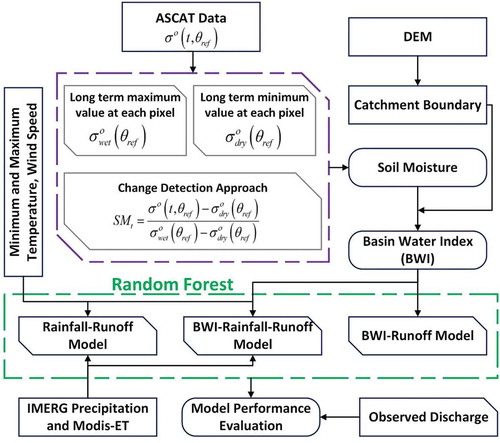
In this study, a relationship is developed between discharge and basin averaged surface soil moisture (basin water index or BWI) using the methodology presented in Fig. 2. The first step in this process is to obtain the watershed of an outlet point (gauging station) from a DEM. The basin delineation was carried out using ArcGIS-10.4 software. Scatterometer-retrieved surface soil moisture, satellite-based precipitation and ET and other climatic parameters for each grid point over the catchment were averaged for the whole catchment. The BWI was compared with the streamflow and utilized for the development of a BWI–runoff model. In addition to this, a classical rainfall–runoff model was developed using satellite-based rainfall, ET and other meteorological parameters (minimum temperature, maximum temperature and wind speed) and compared with the BWI–runoff model. To further investigate the role of soil moisture in hydrological modelling, BWI was integrated with the classical rainfall–runoff model and a BWI–rainfall–runoff model was obtained. Overall, there are three machine learning-based configurations: (1) BWI–runoff model (only BWI was utilized as the input parameter), (2) rainfall–runoff model (satellite-based rainfall, ground-based maximum and minimum temperature, and wind speed were utilized as input parameters), and (3) BWI–rainfall–runoff model (BWI as well as the parameters used for the rainfall–runoff model were utilized as input parameters). Finally, the performance of each model was assessed using observed streamflow. Data pre-processing, model development and plot generation were performed in Python programming language using ascat, scikit-learn, xarray, pandas, numpy, scipy and matplotlib packages.

Figure 2. Flowchart of the methodology for estimation of discharge. ASCAT: advanced scatterometer; DEM: digital elevation model; IMERG: Integrated Multi-satellitE Retrievals for Global Precipitation Measurement; ET: Evapotranspiration

In this study, an ensemble learning algorithm (i.e. a random forest or RF model) was employed for the development of data-driven hydrological models for each station. For the development and assessment of the model performance, the whole dataset was divided into training and testing sets, based on the data available for each station. Training and testing periods for each station are presented in Table 3. Model performance was assessed using three efficiency measures. During the training stage, the best-fit RF model was obtained using the cross-validation technique for each catchment. Further, the model for each catchment was validated using the observed flow, and the performance was evaluated with GloFAS. Moreover, it is well known that the monsoon-dominated catchments in India are highly influenced by the seasonal rainfall. As a result, the seasonal cycle calculated through the average discharge in the different years for each day may produce high performance. Therefore, the performance of the seasonal cycle is assessed with respect to the observed series and compared with the models proposed in this study. The details of the BWI, RF and performance evaluation metrics are presented in the following subsections.

Table 3. Evaluation of BWI–runoff model performance over different river basins using efficiency measures. BWI: basin water index; RMSE: root mean square error; R: correlation coefficient; NSE: Nash-Sutcliffe efficiency

Station	Training period	Testing period	RMSE		R		NSE		Performance rating (Moriasi et al. 2007)
			Training	Testing	Training	Testing	Training	Testing
Kanpur	June 2009–December 2013	January 2014–May 2016	1027.63	453.04	0.95	0.94	0.82	0.53	Satisfactory
Shahijina	January 2007–December 2011	January 2012–May 2014	230.28	984.21	0.96	0.98	0.90	0.86	Very good
Mandleshwar	January 2007–December 2012	January 2013–December 2016	394.59	630.58	0.93	0.95	0.87	0.86	Very good
Basantpur	January 2007–December 2012	January 2013–December 2015	546.99	738.90	0.90	0.84	0.80	0.69	Good
Narsingpur	January 2007–December 2012	January 2013–December 2015	117.47	96.30	0.89	0.73	0.66	0.49	Unsatisfactory
Kollegal	January 2007–December 2012	January 2013–December 2016	119.51	149.78	0.93	0.89	0.79	0.75	Good

3.2.1 Basin water index (BWI)

In this study, to derive the BWI, surface soil moisture $S{M}_t$data were averaged over all grid points of the catchment (Scipal et al. 2005):

(2) $\mathrm{B}\mathrm{W}\mathrm{I}=\frac{{\sum }_{i=1}^n\mathrm{S}{\mathrm{M}}_i}{n}$(2)

Equation (2)(2) $\mathrm{B}\mathrm{W}\mathrm{I}=\frac{{\sum }_{i=1}^n\mathrm{S}{\mathrm{M}}_i}{n}$(2) assumes that all points in the catchment are equally relevant for generation of the runoff (Scipal et al. 2005, Meier et al. 2011). In this approach, the location of each pixel within the watershed area with respect to the gauging site is not considered. It is expected that each pixel shows a unique relation to the hydrometric parameter at the gauging station, specifically in the case of large catchments. After the BWI value was obtained for each catchment, it was compared with the discharge data for the catchment.

3.2.2 Random forest (RF) regression

RF is one of the most popular ensemble learning algorithms and is extensively applied in the field of water resources (Tyralis et al. 2019). As suggested by James et al. (2013), decision tree models such as RF can handle complex relationships between the independent and dependent variables, without any prior assumptions. In water resources, RF belongs to the class of data-driven models (Solomatine and Ostfeld 2008). RF algorithms are stable, flexible and straightforward to use, fast learners compared to other machine learning algorithms and deal well with the overfitting of data, and they can operate in parallel computing mode.

Based on the bootstrap aggregation of regression trees, RF is considered an ensemble learning algorithm. Tyralis et al. (2019) described the RF algorithm as a combination of classification, regression trees and bagging along with some added degree of randomization. The fundamental concept is that all the trees are dependent on a set of random variables and that these trees together form an ensemble forest, which leads to avoiding the problems of overfitting. Considering a training set X = x₁, x₂, …, x_n, responses Y = y₁, y₂, …, y_n, and B times repeated bagging, a random sample (X_b,Y_b) is selected replacing the training set, which is fitted to a regression tree (f_b), for b = 1, 2, …, B.

After training, the unseen samples (say, x’) can be predicted by averaging all the individual regression trees’ predictions on x’ as:

(3) $\hat{f}=\frac{1}{B}{\sum }_{b=1}^B{f}_b\left(x\prime \right)$(3)

This bootstrapping method leads to no increase in bias but a reduction in the variance of the model, thereby improving its performance. The predictions from individual trees may have high sensitivity to noise in the training set, which does not hold for their average provided there is no significant correlation between the trees (Mohsenzadeh Karimi et al. 2020). The uncertainty in the prediction is estimated as the standard deviation of the predictions from all of the single trees on x’:

(4) $\sigma =\sqrt{\frac{{\sum }_{b=1}^B{\left(f_b\left(x^{\prime }\right)-\hat{f}\right)}^2}{B-1}}$(4)

where B is a free parameter, which represents the number of trees. A detailed description of the RF algorithm is given in Breiman (2001).

The procedure applied for the RF model is as follows:

Step 1. Data pre-processing.

Step 2. Separation of data into training and testing sets.

Step 3. Model development and 5-fold cross-validation for hyper-parameter tuning.

Step 4. Model training for the whole training sample using best hyper-parameters.

Step 5. Predicting the discharge using the trained model.

Step 6. Model performance evaluation using efficiency measures (R, NSE, and RMSE; see below).

3.2.3 Model performance evaluation

To evaluate the performance of the model simulations, three widely accepted statistical indices – Nash-Sutcliffe efficiency (NSE), coefficient of correlation (R), and root mean square error (RMSE) – were used. Equations (5)(5) $\mathrm{N}\mathrm{S}\mathrm{E}=1-\frac{{\sum }_{t=1}^N{\left(Q_t^s-Q_t^o\right)}^2}{{\sum }_{t=1}^N{\left(Q_t^o-\overline{Q_{\hspace{0.17em}}^o}\right)}^2}$(5) , (6(6) $R=\frac{{\sum }_{t=1}^N\left(Q_t^o-\overline{Q_{\hspace{0.17em}}^o}\right)\left(Q_t^s-\overline{Q_{\hspace{0.17em}}^s}\right)}{\sqrt{{\sum }_{t=1}^N{\left(Q_t^o-\overline{Q_{\hspace{0.17em}}^o}\right)}^2}\sqrt{{\sum }_{t=1}^N{\left(Q_t^s-\overline{Q_{\hspace{0.17em}}^s}\right)}^2}}$(6) ) and (7(7) $\mathrm{R}\mathrm{M}\mathrm{S}\mathrm{E}=\sqrt{\frac{1}{N}{\sum }_{t=1}^N{\left(Q_t^s-Q_t^o\right)}^2}$(7) ) give the formulae for NSE, R and RMSE, respectively. Krause et al. (2005) and Moriasi et al. (2007) provide a detailed description of these statistical indices, along with their importance and optimum range in hydrological studies. Amongst the three indices, RMSE shows the error associated with the simulated discharge, whereas NSE and R are used to assess the predictive power of a hydrological model (Nash and Sutcliffe 1970) and to assess the degree of linear association between simulated and observed discharge, respectively.

(5) $\mathrm{N}\mathrm{S}\mathrm{E}=1-\frac{{\sum }_{t=1}^N{\left(Q_t^s-Q_t^o\right)}^2}{{\sum }_{t=1}^N{\left(Q_t^o-\overline{Q_{\hspace{0.17em}}^o}\right)}^2}$(5)

(6) $R=\frac{{\sum }_{t=1}^N\left(Q_t^o-\overline{Q_{\hspace{0.17em}}^o}\right)\left(Q_t^s-\overline{Q_{\hspace{0.17em}}^s}\right)}{\sqrt{{\sum }_{t=1}^N{\left(Q_t^o-\overline{Q_{\hspace{0.17em}}^o}\right)}^2}\sqrt{{\sum }_{t=1}^N{\left(Q_t^s-\overline{Q_{\hspace{0.17em}}^s}\right)}^2}}$(6)

(7) $\mathrm{R}\mathrm{M}\mathrm{S}\mathrm{E}=\sqrt{\frac{1}{N}{\sum }_{t=1}^N{\left(Q_t^s-Q_t^o\right)}^2}$(7)

where $Q_t^o$, $Q_i^s$, $\overline{Q^s}$ and $\overline{Q_{\hspace{0.17em}}^o}$ are the observed, simulated, mean simulated and mean observed values, respectively, in time step t, and N represents the total number of observations. The ranges of NSE, R and RMSE values are −∞ to 1, – 1 to 1 and 0 to ∞, respectively, and the optimal values are 1, −1 or 1 and 0, respectively (Motovilov et al. 1999, Moriasi et al. 2007).

4 Results

It is well known that soil moisture plays a key role in the process of runoff generation. Primarily, it can be anticipated that BWI and discharge parameters are interrelated. In other words, when the soil in the catchment is fully saturated or close to the saturation level, the runoff will be higher as compared to the situation when soil is dry, but the relationship between soil moisture and discharge may not be linear. Scipal et al. (2005) and Meier et al. (2011) reported that there exists a logarithmic relationship between BWI and discharge. The integration of soil moisture with the classical rainfall–runoff model may also yield significant results. Therefore, the potential to utilize the scatterometer-retrieved surface soil moisture in hydrological modelling is assessed in the present study. The results of three models (BWI–runoff, rainfall–runoff, BWI–rainfall–runoff) and GloFAS are presented below.

4.1 BWI–runoff model

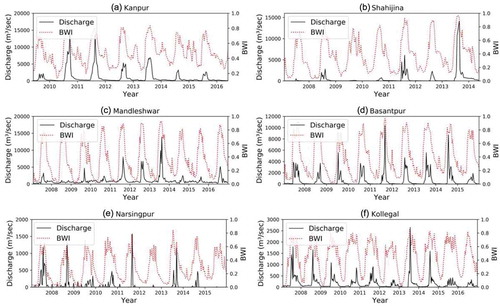
To develop the BWI–runoff model, the pattern of BWI with respect to the observed discharge was assessed from the time series plots for each catchment (Fig. 3). It can be observed that the scatterometer captures the seasonal variation in river discharge very well. In the case of Kanpur station, during the winters, the discharge is very low although BWI shows high values (Fig. 3(a)). This may be due to the application of irrigation as the Rabi season crops are dominant over the catchment area. BWI shows no satisfactory agreement with the discharge over Basantpur and Narasinghpur stations, especially during the wet season (Fig. 3(d) and (e)).

Figure 3. Time series plot of BWI with respect to discharge for (a) Kanpur station, (b) Shahijina station, (c) Mandleshwar station, (d) Basantpur station, (e) Narsingpur station and (f) Kollegal station. BWI: basin water index

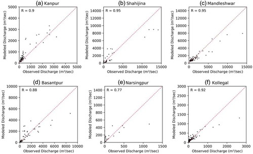
After visual assessment of the BWI time series, the BWI–runoff model was developed for each station. The model performance statistics during the training and testing periods for each station are summarized in Table 3. The scatterplots between observed and modelled discharge for each catchment are presented in Fig. 4. The time series plots of the individual catchments with respect to the observed and modelled discharge for the entire duration are presented in Fig. 5, in which Model-1 represents the BWI–runoff model.

Figure 4. Scatterplots (with 1:1 line) between the observed and modelled discharge (from the BWI–runoff model) during the testing period for (a) Kanpur station, (b) Shahijina station, (c) Mandleshwar station, (d) Basantpur station, (e) Narsingpur station and (f) Kollegal station. R: correlation coefficient; BWI: basin water index

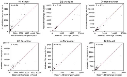
Figure 5. Time series plot of observed and modelled discharge for (a) Kanpur station, (b) Shahijina station, (c) Mandleshwar station, (d) Basantpur station, (e) Narsingpur station and (f) Kollegal station. GloFAS: Global Flood Awareness System; Model-1: BWI-runoff model; Model-2: rainfall-runoff model; Model-3: BWI-rainfall-runoff model; BWI: basin water index

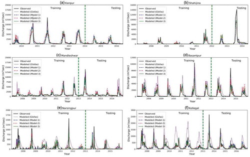
From Fig. 5, it can be observed that the BWI–simulated discharge follows the pattern of the observed discharge very well. The simulations consistently fit the rising limbs, peaks and recession limbs of the observed hydrograph for the training period. The agreement between observed and modelled discharge is unsatisfactory to very good during the testing period, as the values of NSE and R are found to be in the range of 0.49 to 0.86 and 0.73 to 0.98, respectively. Based on the performance evaluation indices (R, NSE and RMSE), the model appeared to be a very good performer for two stations (Shahijina and Mandleshwar), good for two stations (Basantpur and Kollegal), satisfactory for one station (Kanpur) and unsatisfactory for one station (Narsingpur).

From the scatterplots and the time series plots, it can be observed that the peaks are usually underestimated. However, it is overestimated in some of the events (for Kanpur and Kollegal stations). An overestimation of discharge for Kanpur station can be observed for the winter season i.e. January and February months (Fig. 4(a)), which may be attributed to the high soil moisture due to irrigation in the river basin, as mentioned (Fig. 3(a)). One of the reasons for underestimation or overestimation during the testing period may be the difference in ranges of the training and testing samples. It has been observed that during high discharge conditions, the modelled discharges are underestimated, which is reflected in the high values of RMSE. The modelling errors regarding the peak discharge can be attributed to the fact that the discharge is not solely dependent on BWI but depends also on factors such as rainfall, temperature and wind speed that were not considered in this case. However, in general, the models were capable of replicating the hydrological behaviour of the catchments.

4.2 Rainfall–runoff model

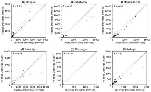
Satellite-based precipitation and ET products are viable sources of data and very important in hydrological studies at regional and global scales, particularly for ungauged catchments in developing countries like India. Despite their superiority over gauge-based ground observations in terms of spatiotemporal resolution, uninterrupted availability and global coverage, satellite data are not commonly integrated into hydrological modelling applications, mainly because documentation of their reliability at larger scales is lacking. The present study evaluates the capability of satellite-based precipitation and ET products for hydrological modelling. The rainfall–runoff model was developed using IMERG precipitation, MODIS ET, maximum and minimum temperature and wind speed for each station. Statistical evaluation of model performance based on 10-d discharge is presented in Table 4. Time series plots and scatterplots comparing the observed and the modelled discharge for each catchment are presented in Figs 5 and 6, respectively. In Fig. 5, Model-2 represents the time series of simulated discharge from the rainfall–runoff model.

Table 4. Evaluation of the rainfall–runoff model’s performance over different river basins using efficiency measures. RMSE: root mean square error; R: correlation coefficient; NSE: Nash-Sutcliffe efficiency

Station	RMSE		R		NSE		Performance rating (Moriasi et al. 2007)
	Training period	Testing period	Training period	Testing period	Training period	Testing period
Kanpur	1209.00	379.29	0.89	0.90	0.75	0.67	Good
Shahijina	247.37	1015.17	0.95	0.95	0.88	0.85	Very good
Mandleshwar	720.43	1134.85	0.82	0.80	0.57	0.55	Satisfactory
Basantpur	383.34	645.45	0.96	0.88	0.90	0.76	Very good
Narsingpur	130.50	92.18	0.82	0.77	0.59	0.53	Satisfactory
Kollegal	119.98	146.12	0.91	0.92	0.79	0.76	Very good

Figure 6. Scatterplots (with 1:1 line) between the observed and modelled discharge (from the rainfall–runoff model) during the testing period for (a) Kanpur station, (b) Shahijina station, (c) Mandleshwar station, (d) Basantpur station, (e) Narsingpur station and (f) Kollegal station. R: correlation coefficient

Based on the statistical evaluation indices, the model performance during the testing period is found to be very good for three stations (Shahijina, Basantpur and Kollegal), good for one station (Kanpur) and satisfactory for two stations (Mandleshwar and Narsingpur). The NSE and R varied from 0.53 to 0.85 and 0.77 to 0.95, respectively, for various stations during the testing period. Like the BWI–runoff models, the rainfall–runoff models mostly underestimated the peaks but overestimated them in some cases (Basantpur and Narsingpur). However, the rainfall–runoff model did not overestimate the winter season events for Kanpur station.

It was observed that the rainfall–runoff model outperformed the BWI–runoff model for three stations (Kanpur, Basantpur and Narsingpur), whereas the performance of the two models was almost the same for two stations (Shahijina and Kollegal). In the case of Mandleshwar station, the BWI–runoff model performed better than the rainfall–runoff model. The results reveal the importance of using satellite-based precipitation and an ET input-specific model for simulating discharge.

4.3 BWI–rainfall–runoff model

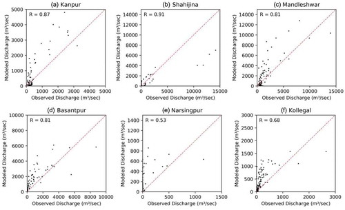
Keeping in view the advantages and limitations of satellite-based soil moisture, rainfall and ET for the hydrological modelling, a new model (the BWI–rainfall–runoff model) was developed with a similar data-driven approach. In this new model, satellite-based soil moisture (BWI), rainfall and ET, and ground-based minimum and maximum temperature and wind speed, were used. Model evaluation statistics for estimating the 10-d discharge are given in Table 5. Time series plots and scatterplots comparing observed and modelled discharge for each catchment are presented in Figs 5 and 7, respectively, where Model-3 represents the time series of simulated discharge from the BWI–rainfall–runoff model.

Table 5. Evaluation of the BWI–rainfall–runoff model’s performance over different river basins using efficiency measures. BWI: basin water index; RMSE: root mean square error; R: correlation coefficient; NSE: Nash-Sutcliffe efficiency

Station	RMSE		R		NSE		Performance rating (Moriasi et al. 2007)
	Training period	Testing period	Training period	Testing period	Training period	Testing period
Kanpur	956.61	346.48	0.94	0.95	0.84	0.72	Good
Shahijina	157.34	916.44	0.98	0.96	0.95	0.87	Very good
Mandleshwar	399.58	608.99	0.93	0.95	0.87	0.87	Very good
Basantpur	495.81	640.95	0.92	0.88	0.84	0.77	Very good
Narsingpur	121.78	91.62	0.85	0.76	0.64	0.54	Satisfactory
Kollegal	98.93	129.59	0.94	0.93	0.86	0.81	Very good

Figure 7. Scatterplots (with 1:1 line) between the observed and modelled discharge (from the BWI–rainfall–runoff model) during the testing period for (a) Kanpur station, (b) Shahijina station, (c) Mandleshwar station, (d) Basantpur station, (e) Narsingpur station and (f) Kollegal station. R: correlation coefficient; BWI: basin water index

The BWI–rainfall–runoff model showed very good performance for four stations (Shahijina, Mandleshwar, Basantpur and Kollegal), good for one station (Kanpur) and satisfactory for one station (Narsingpur), although the peaks were underestimated in some cases. The NSE and correlation between observed and simulated discharge varied from 0.54 to 0.87 and 0.76 to 0.96, respectively, during the testing period.

The BWI–rainfall–runoff model outperformed both the BWI–runoff and rainfall–runoff models. The integration of BWI into the rainfall–runoff model significantly improved the model performance for Kanpur, Shahijina, Mandleshwar and Kollegal stations, whereas the improvement for Basantpur and Narsingpur stations is not significant. From the results, it can be inferred that satellite rainfall products may not perform up to the mark for some of the catchments. However, this limitation may be balanced by the satellite-based soil moisture products. Therefore, the satellite-based soil moisture and rainfall complement each other for hydrological modelling, and their integration results in a better model.

4.4 Comparison of model results with GloFAS discharge

In this study, the GloFAS version-2 river discharge is evaluated for the six catchments of India. The performance evaluation statistics are presented in Table 6. Figures 5 and 8 show the time series and scatterplots, respectively, for each river basin. From these figures, it can be observed that GloFAS generally overestimated the peaks of the hydrograph. GloFAS performance was very good for Kanpur station and good for Shahijina station in simulating the discharge. However, for the other four stations, the performance of the GloFAS model was unsatisfactory. The NSE and correlation between observed and simulated discharge was found to be in the range of −1.12 to 0.81 and 0.54 to 0.91, respectively. When compared with the locally developed hydrological models forced with satellite-based inputs, GloFAS is found to be inferior in accurately estimating the discharge. This is due to the fact that these models were developed at a global scale, and the number of calibration stations may not be sufficient for some regions, leading to its poor performance. In contrast, the models developed here (BWI–runoff, rainfall–runoff and BWI–rainfall–runoff) are region specific. The results indicate that global models may not be suitable for all regions and should be carefully assessed before use in any regional applications.

Table 6. Evaluation of modelled discharge from the global flood awareness system (GloFAS) over different river basins using efficiency measures. RMSE: root mean square error; R: correlation coefficient; NSE: Nash-Sutcliffe efficiency

Station	RMSE			R			NSE			Performance rating (Moriasi et al. 2007)
	Training period	Testing period	Overall	Training period	Testing period	Overall	Training period	Testing period	Overall
Kanpur	989.28	663.31	889.86	0.92	0.87	0.91	0.83	−0.01	0.81	Very good
Shahijina	394.50	1574.85	953.76	0.85	0.91	0.86	0.70	0.63	0.66	Good
Mandleshwar	1267.44	1457.09	1345.00	0.77	0.81	0.79	−0.32	0.27	0.04	Unsatisfactory
Basantpur	1199.16	987.01	1131.38	0.82	0.81	0.81	0.05	0.44	0.20	Unsatisfactory
Narsingpur	203.05	203.31	202.83	0.56	0.53	0.54	0.00	−1.27	−0.22	Unsatisfactory
Kollegal	444.05	334.53	403.20	0.71	0.68	0.69	−1.89	−0.26	−1.12	Unsatisfactory

Figure 8. Scatterplots (with 1:1 line) between the observed and modelled discharge (from GloFAS) during the testing period for (a) Kanpur station, (b) Shahijina station, (c) Mandleshwar station, (d) Basantpur station, (e) Narsingpur station and (f) Kollegal station. R: correlation coefficient; GloFAS: Global Flood Awareness System

4.5 Comparison of model results with seasonal cycle performance

The seasonal precipitation characteristics over the monsoon-dominated catchments of India may be witnessed in the form of seasonal patterns of discharge. Considering the almost sinusoidal trend of the observed discharge (Fig. 5), the seasonal cycle calculated through the average discharge in the different years for each day may produce high performance. Therefore, the seasonal cycle is tested with respect to the observed discharge in terms of efficiency measures, and the results are presented in Table 7. The performance of the seasonal cycle is found to be unsatisfactory over all six catchments. The NSE ranged from −3.79 to 0.37 for the testing period. When compared with the models proposed in this study (i.e. BWI–runoff, rainfall–runoff and BWI–rainfall–runoff), the performance of the seasonal cycle is poor and is always outperformed by the developed models.

Table 7. Evaluation of the discharge seasonal cycle performance over different river basins using efficiency measures. RMSE: root mean square error; R: correlation coefficient; NSE: Nash-Sutcliffe efficiency

Station	RMSE		R		NSE		Performance rating (Moriasi et al. 2007)
	Training period	Testing period	Training period	Testing period	Training period	Testing period
Kanpur	956.61	346.48	0.94	0.95	0.84	0.72	Good
Kanpur	1600.75	1446.15	0.75	0.70	0.57	−3.79	Unsatisfactory
Shahijina	605.11	2558.04	0.55	0.50	0.30	0.03	Unsatisfactory
Mandleshwar	870.83	1545.42	0.62	0.43	0.38	0.17	Unsatisfactory
Basantpur	779.46	1052.86	0.77	0.62	0.60	0.37	Unsatisfactory
Narsingpur	168.33	141.15	0.56	0.45	0.31	−0.09	Unsatisfactory
Kollegal	194.61	260.44	0.67	0.51	0.45	0.24	Unsatisfactory

5 Discussion

The fundamental role of soil moisture is well known; however, with actual observations, contrasting results have been obtained and robust assessment of the worth of satellite soil moisture data in hydrological applications was needed. Machine learning techniques are convenient and economical, require fewer input parameters, and consume less time and effort compared to physically based models, and thus, can be pivotal for developing countries.

The BWI–runoff model was able to capture the seasonal variation; however, it was not able to capture the peaks and it overestimated the discharge in winter seasons (e.g. Kanpur station), which may be due to irrigation activities. The rainfall–runoff model performed quite similarly to the BWI–runoff model, but it was able to resolve the issues of irrigation in the winter season. For most of the catchments, the rainfall–runoff model performed better than or similar to the BWI–runoff model, but sometimes its performance was not as good (e.g. Mandleshwar station). This shows that neither satellite-based soil moisture nor satellite-based rainfall and ET are perfect for hydrological modelling of every catchment. However, one product may complement the other, and a better model may be obtained by integrating them all together. In this regard, the performance of the BWI–rainfall–runoff model was better than that of either the rainfall–runoff model or the BWI–runoff model.

Moreover, the potential of global runoff products (i.e. GloFAS) was also evaluated for discharge prediction over all six catchments. The results revealed the performance of GloFAS to be unsatisfactory over most of the selected catchments. This indicates that the development of region-specific models can be more useful than employing the global runoff products. Further, the seasonal cycle calculated through the average discharge in the different years for each day was also evaluated with respect to the observed series, and the performance was unsatisfactory over all catchments. On the basis of the performances over the catchments, the models can be ranked as follows: BWI–rainfall–runoff > rainfall–runoff > BWI–runoff > GloFAS > seasonal cycle. This general conclusion regarding the performance of the models also applies to Narsinghpur station; however, discharge prediction over this station only ever reached a satisfactory level.

The results are consistent with prior studies (Immerzeel and Droogers 2008, Meenu et al. 2013, Nandi and Reddy 2017, Chanapathi et al. 2018, Adhikary et al. 2019). Nandi and Reddy (2017) that carried out distributed rainfall–runoff modelling over Krishna Basin using a physics-based variable infiltrtaion capacity (VIC) model where the NSE was found to be 0.34 and 0.42 during calibration and validation, respectively. Similarly, application of the Soil and Water Assessment Tool (SWAT) model over the basin by Chanapathi et al. (2018) did not yield very good results with respect to the observed streamflow. Further, Krishna basin is subjected to frequent hydrological extremes (Venkatesh and Singh 1999, Gosain et al. 2006, Gaur et al. 2007), which makes hydrological modelling a great challenge. However, it is necessary to identify the possible improvement options for the catchment, which will be the subject of future work.

The results clearly justify the importance of satellite-based open-access datasets in general, and soil moisture products in particular, for hydrological modelling using ensemble learning techniques. Previous studies (Lee et al. 2011, Lievens et al. 2015, López et al. 2016) on the potential gain of satellite observations for hydrological models agree with the obtained results in the present study. This simulation scheme could perhaps be deemed an alternative for application to ungauged catchments.

6 Summary and conclusions

Most catchments in developing countries are ungauged or have sparsely and unevenly distributed gauging networks. Water management in such cases is quite challenging because of the unavailability of basin-wide gauged hydrological data, whether historical or real time. Under these conditions, a hydrological model forced with satellite-based hydrological fluxes can be effective in estimating the streamflow for water management and decision-making.

The present study was carried out to assess the capability of satellite-based hydrological fluxes for hydrological modelling over six river basins of India. A novel approach was applied to test the value of satellite-based rainfall and ET products for estimation of discharge and, specifically, the significance of satellite-based soil moisture data for the improvement of discharge estimates. The IMERG-precipitation product performed reasonably well for hydrological modelling over four catchments (Kanpur, Shahijina, Basantpur and Kollegal) for the prediction of streamflow.

A comparison of the rainfall–runoff model with the BWI–runoff model showed contrasting results, and the rainfall–runoff model usually performed better than the BWI–runoff model. However, the BWI–rainfall–runoff model outperformed the other two models, and thus, it is best suited for the prediction of 10-d streamflow. The integration of satellite-based soil moisture into the rainfall–runoff model significantly improved the model performance. This implies that soil moisture products can complement the satellite-based rainfall products in simulating discharge. The study also suggests that the locally developed hydrological models forced with satellite-based inputs can be better than global runoff products like GloFAS and that the latter should be carefully assessed before being used in hydrological applications.

The study also demonstrates that further investments and improvements in remotely sensed observations, especially soil moisture products, can benefit large-scale hydrological model predictions. This would provide a global improvement of hydrological simulations, as satellite data often have global coverage. The approach of integrating the satellite-based soil moisture into hydrological models to simulate discharge can be useful, helping in better planning and management of river basins, especially in the developing countries.

Acknowledgements

We would like to thank the Space Applications Centre (SAC), Indian Space Research Organisation (ISRO), Ahmedabad, India, for providing the financial support (Grant No.: ISR-1075-WRC) to carry out this study. The discharge data provided by Central Water Commission (CWC), India, and laboratory facilities provided by the Department of Water Resources Development and Management, IIT Roorkee, are highly appreciated. We extend our sincere gratitude to IMD, H-SAF, ECMWF and NASA for providing open-access data. We are also grateful to Dr Diego Rivera (Associate Editor) and two anonymous reviewers for providing constructive comments to substantially improve the initial version of this paper.

Disclosure statement

No potential conflict of interest was reported by the authors.

Additional information

Funding

This work was supported by the Space Applications Centre, ISRO, Ahmedabad, India [ISR-1075-WRC].

References

- Adhikary, P.P., et al., 2019. Effect of calibration and validation decisions on streamflow modeling for a heterogeneous and low runoff–producing River Basin in India. Journal of Hydrologic Engineering, 24 (7), 05019015. doi:10.1061/(ASCE)HE.1943-5584.0001792.
- Agarwal, A. and Singh, R.D., 2004. Runoff modelling through back propagation artificial neural network with variable rainfall–runoff data. Water Resources Management, 18 (3), 285–300. doi:10.1023/B:WARM.0000043134.76163.b9.
- Alvarez-Garreton, C., et al., 2014. The impacts of assimilating satellite soil moisture into a rainfall–runoff model in a semi-arid catchment. Journal of Hydrology, 519, 2763–2774. doi:10.1016/j.jhydrol.2014.07.041.
- Anjum, M.N., et al., 2019. Assessment of IMERG-V06 precipitation product over different hydro-climatic regimes in the tianshan mountains, north-western China. Remote Sensing, 11 (19), 2314. doi:10.3390/rs11192314.
- Antar, M.A., Elassiouti, I., and Allam, M.N., 2006. Rainfall‐runoff modelling using artificial neural networks technique: a Blue Nile catchment case study. Hydrological Processes: An International Journal, 20 (5), 1201–1216. doi:10.1002/hyp.5932.
- Aubert, D., Loumagne, C., and Oudin, L., 2003. Sequential assimilation of soil moisture and streamflow data in a conceptual rainfall–runoff model. Journal of Hydrology, 280 (1–4), 145–161. doi:10.1016/S0022-1694(03)00229-4.
- Baguis, P. and Roulin, E., 2017. Soil moisture data assimilation in a hydrological model: a case study in Belgium using large-scale satellite data. Remote Sensing, 9 (8), 820.
- Breiman, L., 2001. Random forests. Machine Learning, 45, 5–32. doi:10.1023/A:1010933404324
- Brocca, L., et al., 2010. Spatial‐temporal variability of soil moisture and its estimation across scales. Water Resources Research, 46 (2). doi:10.1029/2009WR008016.
- Brocca, L., et al., 2016. Rainfall estimation by inverting SMOS soil moisture estimates: a comparison of different methods over Australia. Journal of Geophysical Research: Atmospheres, 121 (20), 12–062.
- Brocca, L., et al., 2017. Soil moisture for hydrological applications: open questions and new opportunities. Water, 9 (2), 140. doi:10.3390/w9020140.
- Ceballos, A., et al., 2005. Validation of ERS scatterometer‐derived soil moisture data in the central part of the Duero Basin, Spain. Hydrological Processes: An International Journal, 19 (8), 1549–1566. doi:10.1002/hyp.5585.
- Chanapathi, T., Thatikonda, S., and Raghavan, S., 2018. Analysis of rainfall extremes and water yield of Krishna river basin under future climate scenarios. Journal of Hydrology: Regional Studies, 19, 287–306.
- Chen, S.H., Jakeman, A.J., and Norton, J.P., 2008. Artificial intelligence techniques: an introduction to their use for modelling environmental systems. Mathematics and Computers in Simulation, 78 (2–3), 379–400. doi:10.1016/j.matcom.2008.01.028.
- Chiang, Y.M., et al., 2018. Identifying the sensitivity of ensemble streamflow prediction by artificial intelligence. Water, 10 (10), 1341. doi:10.3390/w10101341.
- Dhami, B., et al., 2018. Evaluation of the SWAT model for water balance study of a mountainous snowfed river basin of Nepal. Environmental Earth Sciences, 77 (1), 21. doi:10.1007/s12665-017-7210-8.
- Dottori, F., et al., 2016. Development and evaluation of a framework for global flood hazard mapping. Advances in Water Resources, 94, 87–102. doi:10.1016/j.advwatres.2016.05.002
- Elshorbagy, A., et al., 2010a. Experimental investigation of the predictive capabilities of data driven modeling techniques in hydrology-Part 1: concepts and methodology. Hydrology and Earth System Sciences, 14 (10), 1931. doi:10.5194/hess-14-1931-2010.
- Elshorbagy, A., et al., 2010b. Experimental investigation of the predictive capabilities of data driven modeling techniques in hydrology-Part 2: application. Hydrology and Earth System Sciences, 14 (10), 1943. doi:10.5194/hess-14-1943-2010.
- Engman, E.T. and Chauhan, N., 1995. Status of microwave soil moisture measurements with remote sensing. Remote Sensing of Environment, 51 (1), 189–198. doi:10.1016/0034-4257(94)00074-W.
- Gaur, A., et al., 2007. Implications of drought and water regulation in the Krishna basin, India. Water Resources Development, 23 (4), 583–594. doi:10.1080/07900620701488513.
- Georgakakos, K.P. and Baumer, O.W., 1996. Measurement and utilization of on-site soil moisture data. Journal of Hydrology, 184 (1–2), 131–152. doi:10.1016/0022-1694(95)02971-0.
- Gosain, A.K., Rao, S., and Basuray, D., 2006. Climate change impact assessment on hydrology of Indian river basins. Current Science, 90 (3), 346–353.
- Gupta, H.V., Sorooshian, S., and Yapo, P.O., 1998. Toward improved calibration of hydrologic models: multiple and noncommensurable measures of information. Water Resources Research, 34 (4), 751–763. doi:10.1029/97WR03495.
- Halff, A.H., Halff, H.M., and Azmoodeh, M., 1993, July. Predicting runoff from rainfall using neural networks. In: C.Y. Kuo, ed. Engineering hydrology. New York, NY: American Society of Civil Engineers, 760–765.
- Harrigan, S., et al., 2020. GloFAS-ERA5 operational global river discharge reanalysis 1979-present. Earth System Science Data, 12 (3), 2043–2060.
- Himanshu, S.K., Pandey, A., and Patil, A., 2018. Hydrologic evaluation of the TMPA-3B42V7 precipitation data set over an agricultural watershed using the SWAT model. Journal of Hydrologic Engineering, 23 (4), 05018003. doi:10.1061/(ASCE)HE.1943-5584.0001629.
- Hirpa, F.A., et al., 2018. Calibration of the global flood awareness system (GloFAS) using daily streamflow data. Journal of Hydrology, 566, 595–606. doi:10.1016/j.jhydrol.2018.09.052
- Houser, P.R., et al., 1998. Integration of soil moisture remote sensing and hydrologic modeling using data assimilation. Water Resources Research, 34 (12), 3405–3420. doi:10.1029/1998WR900001.
- Hsu, K.L., Gupta, H.V., and Sorooshian, S., 1995. Artificial neural network modeling of the rainfall‐runoff process. Water Resources Research, 31 (10), 2517–2530. doi:10.1029/95WR01955.
- Huffman, G.J., et al., 2019. NASA global precipitation measurement (GPM) integrated multi-satellite retrievals for GPM (IMERG). Algorithm theoretical basis document (ATBD). Greenbelt, MD: NASA/GSFC. https://pmm.nasa.gov/sites/default/files/document_files/IMERG_ATBD_V5.1b.pdf.
- Immerzeel, W.W. and Droogers, P., 2008. Calibration of a distributed hydrological model based on satellite evapotranspiration. Journal of Hydrology, 349 (3–4), 411–424. doi:10.1016/j.jhydrol.2007.11.017.
- India-WRIS, 2014. India-water resources information system, river basin reports, version 2.0. http://indiawris.gov.in/wris/#/Basin [Accessed 3 Jan 2020].
- Jackson, T.J., 1993. III. Measuring surface soil moisture using passive microwave remote sensing. Hydrological Processes, 7 (2), 139–152. doi:10.1002/hyp.3360070205.
- James, G., et al., 2013. Statistical learning. In: G. James, et al., eds. An introduction to statistical learning. Springer Texts in Statistics, vol 103. New York, NY: Springer. https://doi.org/10.1007/978-1-4614-7138-7_2
- Kavetski, D., Kuczera, G., and Franks, S.W., 2003. Semidistributed hydrological modeling: a “saturation path” perspective on TOPMODEL and VIC. Water Resources Research, 39 (9). doi:10.1029/2003WR002122.
- Kisi, O., et al., 2012. Intermittent streamflow forecasting by using several data driven techniques. Water Resources Management, 26 (2), 457–474. doi:10.1007/s11269-011-9926-7.
- Kokkonen, T.S. and Jakeman, A.J., 2001. A comparison of metric and conceptual approaches in rainfall‐runoff modeling and its implications. Water Resources Research, 37 (9), 2345–2352. doi:10.1029/2001WR000299.
- Krause, P., Boyle, D.P., and Bäse, F., 2005. Comparison of different efficiency criteria for hydrological model assessment. Advances in Geosciences, 5, 89–97. doi:10.5194/adgeo-5-89-2005
- Lee, H., Seo, D.J., and Koren, V., 2011. Assimilation of streamflow and in situ soil moisture data into operational distributed hydrologic models: effects of uncertainties in the data and initial model soil moisture states. Advances in Water Resources, 34 (12), 1597–1615. doi:10.1016/j.advwatres.2011.08.012.
- Lievens, H., et al., 2015. SMOS soil moisture assimilation for improved hydrologic simulation in the Murray Darling Basin, Australia. Remote Sensing of Environment, 168, 146–162. doi:10.1016/j.rse.2015.06.025
- Liu, Y., et al., 2009. Towards a limits of acceptability approach to the calibration of hydrological models: extending observation error. Journal of Hydrology, 367 (1–2), 93–103. doi:10.1016/j.jhydrol.2009.01.016.
- Loizu, J., et al., 2018. On the assimilation set-up of ASCAT soil moisture data for improving streamflow catchment simulation. Advances in Water Resources, 111, 86–104. doi:10.1016/j.advwatres.2017.10.034
- Londhe, S. and Charhate, S., 2010. Comparison of data-driven modelling techniques for river flow forecasting. Hydrological Sciences Journal–Journal Des Sciences Hydrologiques, 55 (7), 1163–1174. doi:10.1080/02626667.2010.512867.
- López, P.L., et al., 2016. Improved large-scale hydrological modelling through the assimilation of streamflow and downscaled satellite soil moisture observations. Hydrology and Earth System Sciences, 20 (7), 3059–3076. doi:10.5194/hess-20-3059-2016.
- Meenu, R., Rehana, S., and Mujumdar, P.P., 2013. Assessment of hydrologic impacts of climate change in Tunga–Bhadra river basin, India with HEC‐HMS and SDSM. Hydrological Processes, 27 (11), 1572–1589. doi:10.1002/hyp.9220.
- Meier, P., Frömelt, A., and Kinzelbach, W., 2011. Hydrological real-time modelling in the Zambezi river basin using satellite-based soil moisture and rainfall data. Hydrology and Earth System Sciences, 15 (3), 999–1008. doi:10.5194/hess-15-999-2011.
- Mohsenzadeh Karimi, S., et al., 2020. Evaluation of the support vector machine, random forest and geo-statistical methodologies for predicting long-term air temperature. ISH Journal of Hydraulic Engineering, 26 (4), 376–386.
- Moriasi, D.N., et al., 2007. Model evaluation guidelines for systematic quantification of accuracy in watershed simulations. Transactions of the ASABE, 50 (3), 885–900. doi:10.13031/2013.23153.
- Motovilov, Y.G., et al., 1999. Validation of a distributed hydrological model against spatial observations. Agricultural and Forest Meteorology, 98, 257–277. doi:10.1016/S0168-1923(99)00102-1
- Naeimi, V., Bartalis, Z., and Wagner, W., 2009. ASCAT soil moisture: an assessment of the data quality and consistency with the ERS scatterometer heritage. Journal of Hydrometeorology, 10 (2), 555–563. doi:10.1175/2008JHM1051.1.
- Nandi, S. and Reddy, M.J., 2017. Distributed rainfall runoff modeling over Krishna river basin. European Water, 57, 71–76.
- Nash, J.E. and Sutcliffe, J.V., 1970. River flow forecasting through conceptual models part I—A discussion of principles. Journal of Hydrology, 10 (3), 282–290. doi:10.1016/0022-1694(70)90255-6.
- Nayak, P.C., et al., 2013. Rainfall–runoff modeling using conceptual, data driven, and wavelet based computing approach. Journal of Hydrology, 493, 57–67. doi:10.1016/j.jhydrol.2013.04.016
- Njoku, E.G. and Entekhabi, D., 1996. Passive microwave remote sensing of soil moisture. Journal of Hydrology, 184 (1–2), 101–129. doi:10.1016/0022-1694(95)02970-2.
- Pandey, A., et al., 2008. Runoff and sediment yield modeling from a small agricultural watershed in India using the WEPP model. Journal of Hydrology, 348 (3–4), 305–319. doi:10.1016/j.jhydrol.2007.10.010.
- Patil, A. and Ramsankaran, R.A.A.J., 2018. Improved streamflow simulations by coupling soil moisture analytical relationship in EnKF based hydrological data assimilation framework. Advances in Water Resources, 121, 173–188. doi:10.1016/j.advwatres.2018.08.010
- Paulik, C., et al., 2014. Validation of the ASCAT soil water index using in situ data from the international soil moisture network. International Journal of Applied Earth Observation and Geoinformation, 30, 1–8. doi:10.1016/j.jag.2014.01.007
- Prieto, C., et al., 2019. Flow prediction in ungauged catchments using probabilistic Random Forests regionalization and new statistical adequacy tests. Water Resources Research, 55 (5), 4364–4392. doi:10.1029/2018WR023254.
- Rafieeinasab, A., et al., 2014. Comparative evaluation of maximum likelihood ensemble filter and ensemble Kalman filter for real-time assimilation of streamflow data into operational hydrologic models. Journal of Hydrology, 519, 2663–2675. doi:10.1016/j.jhydrol.2014.06.052
- Revilla-Romero, B., et al., 2015. On the use of global flood forecasts and satellite-derived inundation maps for flood monitoring in data-sparse regions. Remote Sensing, 7 (11), 15702–15728. doi:10.3390/rs71115702.
- Running, S., et al., 2019. MOD16A2GF MODIS/Terra net evapotranspiration gap-filled 8-day L4 global 500 m SIN grid V006 [Data set]. NASA EOSDIS Land Processes DAAC. https://doi.org/10.5067/MODIS/MOD16A2GF.006 [ Accessed 14 October 2020].
- Schmugge, T.J., 1983. Remote sensing of soil moisture: recent advances. IEEE Transactions on Geoscience and Remote Sensing, GE-21 (3), 336–344. doi:10.1109/TGRS.1983.350563.
- Scipal, K., Scheffler, C., and Wagner, W., 2005. Soil moisture-runoff relation at the catchment scale as observed with coarse resolution microwave remote sensing. Hydrology and Earth System Sciences, 9 (3), 173–183.
- Silberstein, R.P., 2006. Hydrological models are so good, do we still need data? Environmental Modelling & Software, 21 (9), 1340–1352. doi:10.1016/j.envsoft.2005.04.019.
- Solomatine, D.P. and Ostfeld, A., 2008. Data-driven modelling: some past experiences and new approaches. Journal of Hydroinformatics, 10 (1), 3–22. doi:10.2166/hydro.2008.015.
- Srivastava, A.K., Rajeevan, M., and Kshirsagar, S.R., 2009. Development of a high resolution daily gridded temperature data set (1969–2005) for the Indian region. Atmospheric Science Letters, 10 (4), 249–254.
- Sudheer, K.P., Gosain, A.K., and Ramasastri, K.S., 2002. A data‐driven algorithm for constructing artificial neural network rainfall‐runoff models. Hydrological Processes, 16 (6), 1325–1330. doi:10.1002/hyp.554.
- Suryavanshi, S., Pandey, A., and Chaube, U.C., 2017. Hydrological simulation of the Betwa River basin (India) using the SWAT model. Hydrological Sciences Journal, 62 (6), 960–978. doi:10.1080/02626667.2016.1271420.
- Tan, J., et al., 2019. Diurnal cycle of IMERG V06 precipitation. Geophysical Research Letters, 46 (22), 13584–13592. doi:10.1029/2019GL085395.
- Tang, G., et al., 2020. Have satellite precipitation products improved over last two decades? A comprehensive comparison of GPM IMERG with nine satellite and reanalysis datasets. Remote Sensing of Environment, 240, 111697. doi:10.1016/j.rse.2020.111697
- Tyralis, H., Papacharalampous, G., and Langousis, A., 2019. A brief review of random forests for water scientists and practitioners and their recent history in water resources. Water, 11 (5), 910. doi:10.3390/w11050910.
- Venkatesh, B. and Singh, R.D., 1999. Development of regional flood formula for Krishna basin. ISH Journal of Hydraulic Engineering, 5 (2), 44–54. doi:10.1080/09715010.1999.10514652.
- Wagner, W., et al., 2003. Evaluation of the agreement between the first global remotely sensed soil moisture data with model and precipitation data. Journal of Geophysical Research: Atmospheres, 108 (D19). doi:10.1029/2003JD003663.
- Wagner, W., et al., 2007. Operational readiness of microwave remote sensing of soil moisture for hydrologic applications. Hydrology Research, 38 (1), 1–20. doi:10.2166/nh.2007.029.
- Wagner, W., Lemoine, G., and Rott, H., 1999. A method for estimating soil moisture from ERS scatterometer and soil data. Remote Sensing of Environment, 70 (2), 191–207. doi:10.1016/S0034-4257(99)00036-X.
- Wu, C.L., Chau, K.W., and Li, Y.S., 2009. Predicting monthly streamflow using data‐driven models coupled with data‐preprocessing techniques. Water Resources Research, 45 (8). doi:10.1029/2007WR006737.
- Yaseen, Z.M., et al., 2016. Stream-flow forecasting using extreme learning machines: a case study in a semi-arid region in Iraq. Journal of Hydrology, 542, 603–614. doi:10.1016/j.jhydrol.2016.09.035