Climate change impact and uncertainty analysis on hydrological extremes in a French Mediterranean catchment

ABSTRACT

The Mediterranean region is a climate change hotspot for water resources. However, uncertainty analyses of hydrological projections are rarely quantified. In this study, an in-depth analysis of projections and uncertainties for high and low flows is performed. Climatic projections derived from a recent downscaling method were used, for two representative concentration pathway scenarios (RCPs), five general circulation model/regional climate model (GCM/RCM) couples, three hydrological models (HMs), and 29 calibration schemes. A quasi-ergodic analysis of variance was used to evaluate the contribution of each impact modelling step to the total uncertainty. For high flows, the results show a mean increase of 30% by 2085, and RCPs make the highest contribution to the total uncertainty, followed by GCMs. For low flows, 50% of projections indicate a decrease of 7% or more by 2085, and HM structures, hydrological model parameters, and GCMs are the most important uncertainty sources. These results contribute to raise awareness among water managers regarding future hydrological extreme events.

KEYWORDS:

• hydrological modelling
• climate change
• QUALYPSO
• QE-ANOVA
• uncertainty quantification
• unsolved problems in hydrology (UPH)
• UPH#20
• UPH#21

Editor S. Archfield Associate editor R. Singh

1 Introduction

Climate change impact on water resources is a challenging issue for water managers, as highlighted by the Intergovernmental Panel on Climate Change (Field et al. 2014): “Freshwater-related risks of climate change increase significantly with increasing greenhouse gas concentrations.” (p. 232) This conclusion urges stakeholders and decision makers to think about water management in a new way. The IPCC identifies key risks related to water resources in Europe: an increase in water restrictions due to a strong reduction in water availability combined with an increasing water demand. An increase in the evaporative demand is also expected, which would cause a decrease in runoff, and this pattern is particularly pronounced in southern Europe.

Extreme hydrological events, such as floods and droughts, produce important economic losses, which will increase with climate change. Indeed, droughts cause agricultural and ecological damages: in France in 2018, the total economic loss due to droughts is estimated at €1.5–2 billion (Sénat 2019). Floods have higher impacts on urban lands and endanger people living in areas of potential flood risk, resulting in a mean annual cost of €520 million in France (CGDD 2019). Furthermore, the Mediterranean region is described as a climate change hotspot (Diffenbaugh and Giorgi 2012), where hydro-hazards (floods and droughts) will intensify with climate change (Edenhofer et al. 2011). For instance, the intensity of heavy precipitation events will become stronger in the Mediterranean basin, as the 95th percentile of daily rainfall is expected to increase by 20% (Guiot and Cramer 2016). Similarly, the mean change in the 20-year return period of extreme precipitation is expected to increase by around +5% in the French Hérault River catchment by the end of the 21st century (Tramblay and Somot 2018). Moreover, drought events will become longer and more severe in various Mediterranean catchments (Sellami et al. 2016, Marcos-Garcia et al. 2017, Marx et al. 2018), as projected for example by the Standardized Precipitation Index in southern France between 2070 and 2100 (Hertig and Tramblay 2017).

An essential task in hydrological impact studies is the estimation of the different sources of uncertainty (Hattermann et al. 2017), namely uncertainty due to the greenhouse gas emission scenario, uncertainty due to the different models (climate models, hydrological models) used in the chain to simulate the unknown future regarding e.g. hydro-hazards (Mitchell and Hulme 1999), and uncertainty due to the natural variability of the climate. These different uncertainty sources result in a wide range of possible climate change impact projections. Evaluating uncertainties in a multi-model approach is now becoming the norm (Kundzewicz et al. 2008, Hawkins and Sutton 2009, 2011). Empirical approaches have been widely used to explore, one by one, sources of uncertainty and rank them (see e.g. Kay et al. 2009, Dobler et al. 2012). More formal analysis of variance (ANOVA) methods have been used in recent years (e.g. Yip et al. 2011, Addor et al. 2014, Hingray and Saïd 2014, Parajka et al. 2016). Applied to multiscenario multimodel ensembles of experiments, ANOVA approaches allow for a statistically sound partitioning of the different uncertainty sources and of their relative contributions to the total uncertainty. The sources of uncertainty frequently quantified with the ANOVA approach are representative concentration pathway scenarios (RCPs), general circulation models (GCMs), and the internal variability of climate. Other sources can be investigated for a climate impact study. For example, Lafaysse et al. (2014) quantified the relative contributions of general circulation models and of the downscaling step, and Vidal et al. (2016) quantified the uncertainty produced in addition by hydrological models.

ANOVA approaches have been developed to partition uncertainty sources in climate projection ensembles. Most of them are based on a single time analysis, where the only projections available for the considered future period are considered for the uncertainty estimation (e.g. Addor et al. 2014, Parajka et al. 2016). Another option is a time series approach, where all the data from the available climate experiments are used for uncertainty estimation (e.g. Hawkins and Sutton 2009, Hingray and Saïd 2014). The precision of uncertainty quantification obtained with a time series approach has been estimated to be much higher than that for a single time approach, the latter potentially leading to large errors in all uncertainty component estimates (Hingray et al. 2019).

In all cases, a potentially critical issue in uncertainty analysis is that of missing climate model runs, which typically makes the climate projection ensembles incomplete (Déqué et al. 2007, 2012, Evin et al. 2019). Climatic projections are generally missing for some combinations of models and scenarios. In this case, standard estimation methods can lead to biased estimates of ANOVA parameters. To tackle this issue, Evin et al. (2019) developed the quasi-ergodic analysis of climate projections using data augmentation (QUALYPSO) method, which is designed to deal with an incomplete dataset (i.e. the lack of some combinations of models and scenarios). QUALYPSO merges the analytical frameworks of the QE-ANOVA method, a time series ANOVA approach that assumes quasi-ergodicity of transient climate projections (Hingray and Saïd 2014), and of Bayesian data augmentation techniques, which allows coping with missing data.

Mediterranean catchments are known to be vulnerable to extreme floods and flash floods, as the region is exposed to heavy rainfall, and these are referred to as “Mediterranean events” (Thiébault and Moatti 2018). Moreover, the regional climate is vulnerable to severe droughts, and management of the water resources is crucial to satisfy the increasing water demand (Milano et al. 2012). With the impact of climate change on this region, it is essential to evaluate changes in hydrological extremes. In this context, the IPCC recommends adopting more flexible management strategies, and anticipating planning according to different scenarios, to foster resilience to uncertain hydrological futures. Until now, water management plans have usually been based on observed hydrological records from gauging stations. However, to build suitable strategies to climate change impact, water managers need hydrological projections, that might show a high degree of uncertainty (inherent to modelling processes), which makes interpretation of projections challenging. Improving the partitioning of the uncertainty, and better communication with stakeholders, is key to take decisions in an uncertainty context (Refsgaard et al. 2013).

Hydrological projections are produced through impact modelling chains to quantify climate change impacts on water resources (Post et al. 2012, Haddeland et al. 2014, Lespinas et al. 2014, Schewe et al. 2014), hydro-hazards (Collet et al. 2017), and low flows (Piras et al. 2014) at the local and regional scale. The regional challenges are particularly tangible in the Hérault River catchment of southern France (http://www.fleuve-herault.fr/). According to a recent regional water management report (www.eaurmc.fr, 2014), this catchment shows high vulnerability to climatic and anthropogenic changes (Collet et al. 2015). Since this catchment shows high needs and challenges in terms of water management, it has been a focus of attention in prospective studies (Chauveau et al. 2013, Milano et al. 2013, Collet et al. 2015). For example, Collet et al. (2015) evaluated water sustainability through an impact modelling chain and concluded that under a non-mitigation scenario, water resource sustainability will be strongly reduced; as a consequence, reflections on more suitable water restrictions are now being developed. However, the high magnitude of uncertainty related to the hydro-climatic projections causes difficulties in interpreting results and selecting the best adaptation strategy (Fabre et al. 2016).

The need to evaluate and understand changes in the water cycle caused by climate change is highlighted by the work of Blöschl et al. (2019), who remind readers of current fundamental issues for hydrological research. The present work aims to contribute to reflections on unsolved problems in hydrology (UPH) 20: “How can we disentangle and reduce model structural/parameter/input uncertainty in hydrological prediction?” and 21: “How can the (un)certainty in hydrological predictions be communicated to decision makers and the general public?” Thus, the main objective of this study is to investigate and evaluate sources of uncertainty that contribute to the total uncertainty of future streamflow projections. The main research question is whether the uncertainty from global and regional climate models and different greenhouse gas emission scenarios is larger than the uncertainty from the structure and calibration methods of hydrological models. The assessment of the relative contribution of different sources of uncertainty is compared for future projection of low and high flows in a Mediterranean catchment.

2 Material and methods

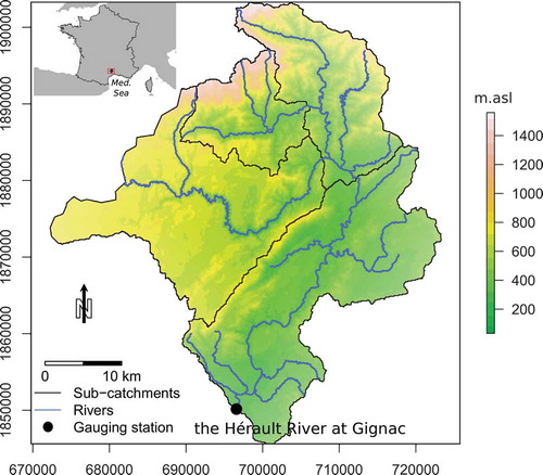
2.1 Study area: the Hérault River catchment

The Hérault River is located is located in Southern France, draining to the Mediterranean Sea in Agde. In this study, only the catchment area upstream of the Gignac gauging station was considered, since there is little urban area and it is considered a near-natural catchment (see Fig. 1). The basin is delimited in the north by the Cévennes mountain range. It is characterized by fractured bedrock and forest cover on the upstream part, and by a karst system on the downstream part of the considered catchment area. The hydrological dynamics are typical for Mediterranean catchments, with intense precipitation influence from the Cévennes Mountains in spring and autumn, and a highly contrasting spatial distribution of annual precipitation (from more than 1500 mm/year upstream to less than 600 mm/year downstream). In terms of temperature, the regional mean is mild in winter (above 5°C), whereas summers are dry and hot (above 20°C), and temperatures are higher downstream and lower upstream.

Figure 1. The Hérault River catchment

Med. Sea: Mediterranean Sea.

2.2 Observed hydro-climatic data

Observed hydro-climatic data used in this work come from the hydro-Système d’Analyse Fournissant des Renseignements Atmosphériques à la Neige (SAFRAN) daily dataset (Delaigue et al. 2019), for which climate datasets from 1958 to 2018 come from the SAFRAN meteorological reanalysis (Vidal et al. 2010) and streamflow series come from the Banque Hydro database (Leleu et al. 2014). The climatic variables include temperature, precipitation, and potential evapotranspiration (PET). In this study, the Penman-Monteith PET formula (Monteith 1965) was used. Streamflow records were available at the daily time step, from 1992 to 2018 for the Gignac station and from 1990 to 2018 for the other stations (see Fig. 1 for station locations). These records were used to calibrate the hydrological models.

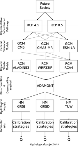
2.3 Climatic projections

To investigate climate change impacts on hydro-hazards and quantify the related uncertainties in this work, several greenhouse gas emissions scenarios (RCPs) and models (climatic and hydrological) were used, which allowed a characterization and a ranking of the diverse uncertainty sources using the QUALYPSO method described in Section 2.6. Five GCM/RCM (general circulation model/regional climate model) couples from coordinated downscaling experiment – European domain (EURO-CORDEX; Jacob et al. 2014) were available for climatic projections; they were downscaled with the ADAMONT method by Météo-France (Verfaillie et al. 2017). ADAMONT uses outputs from RCMs, draws a new grid at a higher spatial resolution (8 km) and includes a statistical bias correction method combined with a weather-type approach. ADAMONT is based on the well-known quantile mapping approach, and it is coupled to the analogous method, to identify various weather patterns, so ADAMONT projections consider the future climate as a modification of the weather pattern frequency. The driving GCMs used in the study are CNRM-CM5, IPSL-CM5A-MR, MPI-ECM-LR; and the RCMs are RCA4, WRF331F, and ALADIN53. Not all GCM/RCM combinations were available (see Table 1). The management of this incomplete set will be further discussed in the uncertainty analysis. The low number of couples at our disposal, compared to the existing EURO-CORDEX ensembles, is explained by the computing cost of the downscaling step with ADAMONT. Two different RCPs are available for each GCM/RCM couple (RCP4.5 and RCP8.5). Climatic projections include the same daily climatic variables as SAFRAN, for the 1970–2100 period. The time period 1976–2005 was defined as the baseline, i.e. a period in which all scenarios are forced by the same observed greenhouse gas emissions; it is referred to as the reference period in this analysis.

Table 1. Matrix of available general circulation model/regional climate model (GCM/RCM) couples

RCM/GCM	CNRM-CM5	IPSL-CMA5-MR	MPI-ESM-LR
ALADIN53	×
WRF331F		×
RCA4	×	×	×

2.4 Hydrological modelling

Three different bucket-type hydrological models (HMs) were used in a multi-model approach. Modèle du Génie Rural à 5 paramètres Journalier (GR5J; Pushpalatha et al. 2011) is a lumped model with five parameters, which has already been used in impact studies (e.g. Sauquet et al. 2016). GR5J was used with the airGR R package (Coron et al. 2017, 2019). Technische Universität Wien (TUW; Parajka et al. 2007) is another lumped model, with 15 parameters, also used for impact studies (Parajka et al. 2016). TUW was used with the TUWmodel R package (Viglione and Parajka 2019). Semi-distributed GR model (GRSD; De Lavenne et al. 2019) is a semi-distributed model, with seven parameters, that was also applied to climate change impact studies (Thirel et al. 2019). It is important to note that several past studies in this basin mainly used conceptual lumped models (e.g. Fabre et al. 2016, Grouillet et al. 2016), which is in line with our choice to use only conceptual models. In addition, the chosen models have already been used with satisfactory results in larger basins than the Hérault catchment (see De Lavenne et al. 2019 for application of GRSD over the whole of France, Dorchies et al. 2014 for application of a lumped GR model over the Seine catchment, and Parajka et al. 2016 for application of TUW over all of Austria).

Different calibration procedures were used to generate 29 parameter sets and assess the uncertainties related to the hydrological model parametrization. This source of uncertainty is usually ignored, although it can be a major factor of influence on hydrological projections (see Parajka et al. 2016, Vidal et al. 2016). The 29 calibration periods were defined and inspired by various options proposed in the literature, as summarized by Thirel et al. (2015). The aim was to represent as diverse a set of conditions as possible, to quantify the model parameter-related uncertainty. The following periods were used for the three hydrological models:

• The whole calibration period was used (1992–2018, one calibration period).

• The whole period was divided into two parts of equal length.

• Two contrasting periods, the wettest and the driest (note that wet and dry periods are short), were used, which allows the evaluation of uncertainties due to climate contrast between the two periods. These periods were built based on the cumulative sum of monthly precipitation anomaly (two calibration periods).

• The rolling calibration approach: models were calibrated on a 10-year period, then this period was moved 1 year forward (19 calibration periods).

• k-fold cross-validation: the record was divided into n parts (with n = 5), where n − 1 parts are used to calibrate the model (five calibration periods).

For each calibration experiment, a 2-year warm-up period was used for initialization of the models’ internal variables. When part of the 1992–2018 period was used for calibration, the rest was always used for performance evaluation. Note that the calibration period (1992–2018) is different from the baseline period (1976–2005) used as a reference for climate change impact quantification. This is due to the observed streamflow series availability (from 1992 in Gignac), the need to calibrate the hydrological models on a 20- to 30-year time period for impact studies (hence using the longest record as possible), and the fact that historical GCM/RCM hindcasts stop in 2005 while needing a 30-year reference time in the past time period. An objective function (OF) that allowed a fair compromise of both low and high flows was chosen. This objective function relies on the Kling-Gupta Efficiency (KGE, Gupta et al. 2009). The average KGE value, calculated with discharge and inverse of discharge series, was used to represent both high and low flows:

(1) $OF=\frac{KGE\left(Q\right)+KGE\left(\frac{1}{Q}\right)}{2}$(1)

The complete procedure is summarized in the following flowchart (Fig. 2).

Figure 2. Flowchart of the cascade of uncertainties, based on the method used in this study

2.5 Hydrological indicators

Hydrological projections were produced from 1976 to 2100. These projections were analysed using a set of indicators focusing on either high or low flows. These indicators were calculated for each year from 1976 to 2100. For high flows, a threshold defined as the 95th percentile of daily discharge (a streamflow value exceeded 5% of the time, Q95), was computed, for each year. For low flows, the mean annual 7-d minimum flow (MAM7) was computed. MAM7 is a commonly used hydrological indicator, well correlated to low flows for climate impact studies (Bauwens et al. 2011, Vidal et al. 2016), whose annual resolution is adapted to study yearly anomalies. For each hydrological indicator and each modelling chain, a 30-year rolling mean plus a spline fitting was computed. The climate response of the 30-year mean variable, estimated with a trend model fitted to the data (see next section), was then used to estimate for each projection lead time the future changes (relative anomaly) expected for the 30-year means and their internal variability. Hydrological indicator projections are therefore presented in terms of anomaly, i.e. the change between the baseline and the future periods, for both hydrological extremes, and results are shown with a 90% confidence interval.

2.6 Uncertainty analysis

The uncertainty here comes from different sources, namely RCPs, GCMs, RCMs, HMs, hydrological model parameters, and internal variability. The uncertainty from these various sources was estimated using the QUALYPSO method (Evin et al. 2019) in the QUALYPSO R package (Evin 2019). To obtain a robust estimation of uncertainty, the use of a complete multi-scenario multi-model ensemble of climate projections (MME) is recommended. Not all combinations of models are available for the MME considered in the present study, as shown in Table 1. This issue is tackled by the QUALYPSO method using a Bayesian setting including data augmentation techniques (International Environmental Modelling and Software Society 2012) to properly treat these incomplete ensembles. The QUALYPSO model is then applied to a full matrix of modelling chains, filled in with Bayesian inference.

The main steps of QUALYPSO are as follows. Note first that a model chain is a single pathway from the top of the modelling chain (RCP) to the bottom (hydrological model parametrization), through each modelling step (namely GCM, RCM, downscaling, and hydrological model), using one model at each modelling step. In other words, it represents the model cascade used to obtain one member of the projection ensemble. The climate response of each model chain is first estimated with a smoothing spline fitted to the 30-year rolling means of the hydrological indicators obtained from the raw projections (i.e. raw hydrological model outputs based on climatic projections). The climate response for the control period is the value of the fitted spline for the control period, and similarly for the future period. For each chain, the variance of the fluctuations from the climate change response of the chain gives an estimate of the internal variability of the chain. The internal variability variance of the MME is estimated as the mean value of the internal variability variances obtained for the different model chains. The climate responses of the different chains are then used to estimate the different scenario/model uncertainty components of the MME. However, the ANOVA makes an additive decomposition: for a given future period, the climate change response of a given chain is assumed to be the sum of the main effects for that period of the different scenarios/models considered in the chain. GCM uncertainty was estimated as the variance of the dispersion between the mean climate change responses obtained for the different GCMs over all hydro-climatic experiments. The same is applied to estimate the uncertainty variances due to the RCP, the RCM, and the hydrological model.

Note, however, that the uncertainty due to hydrological models is divided here into the uncertainty due to the structure of the models (three different models) and the uncertainty due to the parametrization of the models (29 parametrizations as a result of the 29 different periods used for the calibration of each model), namely the hydrological model parameter uncertainty. The hydrological model structure uncertainty is here estimated from the dispersion between the inter-parametrization mean responses of the three different model structures (for each model, the mean response is the mean of the 29 responses obtained from the 29 model parametrizations). The hydrological model parameter uncertainty is estimated from the 29 parametrizations (for each model, it is estimated from the dispersion among the 29 responses of the 29 model parametrizations; for the MME, it is simply estimated as the mean of these estimates). Note also that a part of the dispersion between the climate responses of the different modelling chains cannot be explained by the additive uncertainty decomposition assumed by the method. This leads to residuals in the ANOVA model. The residual variance, i.e. the variance of the ANOVA residuals, is also quantified within QUALYPSO. It can be partly due to interactions between models/scenarios (e.g. Hingray and Saïd 2014). The total uncertainty variance of the MME is, finally, the sum of all uncertainty components, as defined above. It has the following expression:

(2) ${\sigma }_{\mathrm{t}\mathrm{o}\mathrm{t}}^2\left(t\right)={\sigma }_{\mathrm{R}\mathrm{C}\mathrm{P}}^2\left(t\right)+{\sigma }_{\mathrm{G}\mathrm{C}\mathrm{M}}^2\left(t\right)+{\sigma }_{\mathrm{R}\mathrm{C}\mathrm{M}}^2\left(t\right)+{\sigma }_{\mathrm{H}\mathrm{M}}^2\left(t\right)+{\sigma }_{\mathrm{p}\mathrm{a}\mathrm{r}}^2\left(t\right)+{\sigma }_{\mathrm{i}\mathrm{n}\mathrm{t}.\mathrm{v}\mathrm{a}\mathrm{r}.}^2\left(t\right)+{\sigma }_{\mathrm{r}\mathrm{e}\mathrm{s}}^2\left(t\right)$(2)

with t being the future projection period, σ²_tot the total variance, σ²_RCP the variance associated with RCPs, σ²_GCM the variance associated with GCMs, σ²_RCM the variance associated with RCMs, σ²_HM the variance associated with hydrological models, σ²_par the variance associated with hydrological model parameters, σ²_int.var. the variance associated with the internal variability, and σ²_res the residual variance.

In this study, we discuss the time evolution of the total uncertainty variance associated with both high- and low-flow indicators, along with the proportion of variance associated with each uncertainty source. Moreover, the mean effects of each scenario and climate model (GCMs and RCMs separately) can be explored and compared, allowing us to identify the models that induce the highest or lowest changes, and the models that contribute the most to the different uncertainty components.

3 Results

3.1 Precipitation projections

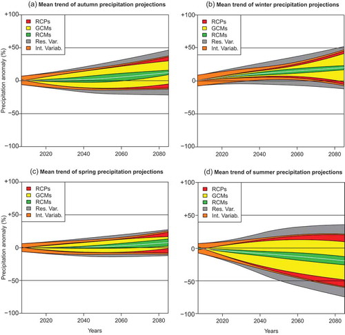
Prior to investigating future hydrological responses to climatic projections, changes in seasonal precipitation are explored to understand the uncertainty in hydrological projections. The mean trend and associated uncertainty ranges of precipitation projections constrain the hydrological models the most, and changes in low and high flows are particularly tied to changes in precipitation, as discussed below. Specifically, high flows are sensitive to changes in spring and autumn precipitation, while low flows occur mainly during summer and are sensitive to both summer precipitation and the groundwater contribution.

Figure 3 shows changes in the mean trend and uncertainty in the seasonal precipitation anomaly for autumn (Fig. 3(a)), winter (Fig. 3(b)), spring (Fig. 3(c)), and summer (Fig. 3(d)). The uncertainty sources are related to RCPs (in red), GCMs (in yellow), RCMS (in green), the internal variability (in orange), and the residual uncertainty (in grey). By 2085, autumn, winter, and spring precipitation show a mean increase of +7% to +18.5%, while summer precipitation decreases by −20% on average. The uncertainty bounds are the largest for summer precipitation projections (from −74% to +33%), followed by autumn (from −22.5% to +46%), winter (from −13% to +56%), and finally spring (from −12% to +27%). There is thus a mixed message here, that although seasonal precipitation shows a mean increasing trend, it is still likely that it would decrease, contrary to temperature projections (not shown here) that show a consistent mean increase of +2.5°C (to +5°C). GCMs provide the main contribution to variance (to 57% by 2085) in autumn, winter, and summer, while for spring precipitation this shifts at the long lead time when variance is mainly related to RCPs (35%) and RCMs (27%). The dominant contribution of GCM and RCM uncertainties for seasonal precipitation in the Mediterranean region, and more generally over Europe, has been clearly shown by Déqué et al. (2012). The residual uncertainty is non-negligible and is up to 24% for summer precipitation changes. It is also the case for the hydrological variables assessed in this study. We discuss this point further in Section 4.

Figure 3. Expected changes and uncertainties in the spline fit to the 30-year rolling mean seasonal precipitation: grand ensemble mean expected trend with 90% confidence intervals in (a) autumn (September–November), (b) winter (December–February), (c) spring (March–May) and (d) summer (June–August). The contribution of each uncertainty source to the total uncertainty is indicated by the different colour bands. Res. Var.: residual variability; Int. Variab.: internal variability

3.2 Low flow projections

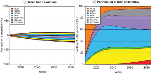
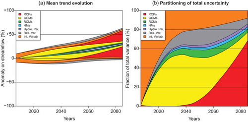
Figure 4(a) shows the mean trend of changes in the 30-year rolling-mean low flows (MAM7 indicator). The mean trend presents a small decrease over time to reach −7% by 2085 compared to the baseline. However, the confidence interval (from −24% to +12%) covers both negative and positive anomalies, and indicates a large uncertainty in low-flow future trends on the Hérault River catchment. Figure 4(b) shows the relative uncertainty components (RCPs, GCMs, RCMs, HMs, HM internal parameters, and internal variability) associated with low-flow projections. The part of the residual error is non-negligible, around 11.5% by 2035 onward. The major uncertainty sources are HMs, hydrological parameters, and GCMs, which represent 29%, 24%, and 20%, respectively, of the total uncertainty by 2085. The contributions of RCPs, RCMs, and the internal variability to the total uncertainty are minor (less than 16% each). The contribution of the different effects changes over time, but after 2025 the contribution of each factor as described above remains stable. Clearly, for this variable, the major part of the total uncertainty is related to the hydrological modelling step. These contributions are further discussed in Section 4.1.

Figure 4. Expected changes and uncertainties in low flows (spline fit to the 30-year rolling mean of the yearly mean annual 7-d minimum flow, MAM7): (a) 90% confidence intervals of the mean change, and (b) relative contribution of the different uncertainty sources to the total uncertainty. Hydro. Par.: hydrological model parameters; Res. Var.: residual variability; Int. Variab.: internal variability. Control period: 1976–2005

3.3 High-flow projections

Figure 5(a) shows the mean trend of changes in high flows (Q95 indicator). It shows a high increase over time to reach +30% by 2085 compared to the baseline. The major part of the confidence interval covers positive anomalies (from −1% to +64% by 2085). The part of the residual error explaining the total uncertainty is small (Fig. 5(b)), around 6.5%. The model contributions explain the total uncertainty by 2085 in the following order: RCPs (69%), GCMs (8%), internal variability (8%), RCMs (3%), HMs (3%), and finally hydrological model hydrological parameters (2.5%). The contribution of each uncertainty source changes over time: in the short lead time (2035), the internal variability represents 25%, and GCMs and RCMs together contribute 59% of the total uncertainty, while in the far lead time (2085) the contribution of these factors decreases.

Figure 5. Expected changes and uncertainties in high flows (spline fit to the 30-year rolling mean of the yearly Q95): (a) 90% confidence intervals of the mean change, and (b) relative contribution of the different uncertainty sources to the total uncertainty. Hydro. Par.: hydrological model parameters; Res. Var.: residual variability; Int. Variab.: internal variability. Control period: 1976–2005

3.4 Analysis of climatic scenario and climate model effects

Figure 6 shows the relative trends of climatic scenarios (RCP, left column), GCMs (middle column), and RCMs (right column), based on the absolute difference of temperature projections (Fig. 6(a,b,c)), and on the relative difference of autumn precipitation (October–December) (Fig. 6(d,e,f)), spring precipitation (March–May) (Fig. 6 (g,h,i)), summer precipitation (June–August) (Fig. 6 (j,k,l)), and PET projections (Fig. 6(m,n,o)). The effects of climatic scenarios and models are compared to each other, to assess changes for the different variables (temperature, precipitation) provided by each model, and to quantify the differences between models relative to the mean value. For instance, in Fig. 6(a), the projected temperature by 2085 with RCP8.5 is 1°C higher than the mean projected temperatures, and vice versa: the temperature projected with RCP4.5 is 1°C lower than the mean projected temperature.

Figure 6. Main effects of the different RCPs (left column), GCMs (middle column), and RCMs (right column) on climatic projection changes for projections of annual temperature (a, b, c), autumn precipitation (d, e, f), spring precipitation (g, h, i), summer precipitation (j, k, l), and annual PET (m, n, o). Solid lines represent the mean effect of each climate scenario or model; the 90% confidence interval of QUALYPSO estimations is drawn in shaded color

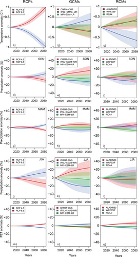
RCPs 4.5 and 8.5 (left column) show clear divergence for all climatic variables, with RCP8.5 inducing a change in precipitation below the average (15% below the ensemble mean of summer precipitation, Fig. 6(j)) and a higher increase in temperature and PET (5% above the ensemble mean) compared to RCP4.5 (Fig. 6(a,m)). For the three GCMs (middle column), a high magnitude of differences in precipitation projections is computed: summer precipitation (Fig. 6(k)) shows a clear divergence of pathways for each GCM (CNRM-CM5 is 25% higher and IPSL-CMA5-MR is 20% lower than the mean projections), as does autumn precipitation (Fig. 6(e)), while spring precipitation (Fig. 6(h)) shows a smaller divergence between GCMs. For the three RCMs (right column), autumn and summer precipitation projections have large and overlapping confidence intervals (Fig. 6(f,l)), and no clear distinction between them can be drawn; spring precipitation projections have smaller overlapped confidence intervals (Fig. 6(i)), while PET projections show a clear divergence between RCM ALADIN53 (+6.5%) and the other two (−1%, and −5.5%) (Fig. 6(o)).

Figure 7 shows the relative changes in high- and low-flow projections, comparing, from left to right, RCPs, GCMs, RCMs, HMs, and HM parameter contributions. High flows show a high divergence related to RCPs (Fig. 7(a)). Regarding GCMs (Fig. 7(b)), high-flow projections show a similar dynamic to autumn precipitation, with MPI-ESM-LR staying below the mean while the other two converge by the end of the 21st century. For RCMs (Fig. 7(c)), the confidence intervals for high-flow projections are overlapping, with a small divergence, which is similar to autumn precipitation. The divergence of HMs is small compared to the others (Fig. 7(d)), with GR5J hydrological projections above the mean (+4%) and TUW below (−4%). The same observation is made for hydrological model parameters (Fig. 7(e)). The major and clear divergences between RCPs and GCMs on autumn precipitation, which are driving processes to high flows, lead these models to contribute the most to uncertainty in high-flow projections.

Figure 7. Main effects on hydrological projections of RCPs, GCMs, RCMs, HMs, and hydrological model parameters on high flow (a, b, c, d, e) and low flow (f, g, h, i, j) projections. Solid lines represent the mean effect of each climate scenario or model; the 90% confidence interval of QUALYPSO estimations is drawn in shaded colour. For parameters, each line represents a parameter set calibrated on a specific period for the three HMs

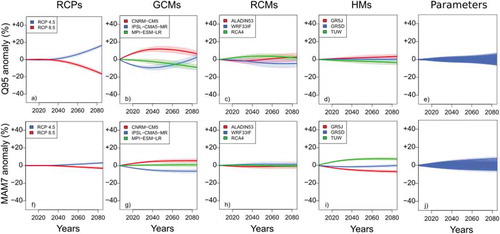
Regarding low-flow projections (bottom row), GCMs (Fig. 7(g)) show a constant difference between models over time. This result is comparable to summer precipitation differences according to GCMs (Fig. 6(k)). HMs show similar orders of differences (Fig. 7(i)), as TUW simulates higher low flows than the mean (+6%), and GR5J simulates lower low flows than the mean projections (−6%). These observations are consistent across the modelling chain for summer precipitation projections: IPSL-CMA5-MR is the GCM that provides changes in summer precipitation and low-flow projections below the mean, while CNRM-CM5 induces changes in summer precipitation and low flow projections above the mean. Moreover, hydrological model parameters (Fig. 7(j)) show the same magnitude of uncertainty as HMs. This shows that hydrological model parameters are also an important source of uncertainty that need to be accounted for in hydrological impact studies. RCPs and RCMs, in contrast, have a small effect on low-flow projections, but a major effect on PET projections. Low-flow projections for this catchment seem less sensible to evapotranspiration rising (which would be linked to rising temperature), and rather more to summer precipitation.

To conclude, the analysis of spring and autumn precipitation shows that GCMs and RCPs have the most divergent effects (Fig. 6), but RCPs become divergent later than GCMs. For these reasons, GCMs are the main source of uncertainty for autumn and spring precipitation at the mid lead time, and RCPs are the main source at the end of the 21st century (Fig. 3(a,c)). This cascades into high-flow projections that show the same ranking of uncertainty sources: GCMs at the mid lead time and RPCs at the long lead time (Fig. 5(b)).

Similarly, summer precipitation show an important divergence for RCPs (Fig. 6(j)), but GCMs are more divergent (Fig. 6(k)), which explains why they provide the main uncertainty contribution to summer precipitation projections (Fig. 3(d)). As a consequence, low-flow projections present the same ranking of uncertainty sources as summer precipitation for climate modelling, with GCMs inducing the largest variance (Fig. 7 (g)). However, HMs (Fig. 7(i)) and hydrological model parameters (Fig. 7(j)) induce a larger variance than GCMs in low-flow projections, which explains that these three components of the modelling chain (from the top down: HMs, hydrological model parameters, and GCMs) are the main contributors to the total uncertainty here.

Note that the 29 hydrological parameter sets could artificially increase the number of chains, which could reduce the contribution of the GCMs/RCMs. This point could lead to an underestimation of the confidence intervals represented in Fig. 7. To test this, it could be interesting to use QUALYPSO with fewer parameter sets.

4 Discussion

4.1 Performance and robustness of hydrological models

To better understand the simulated changes in hydrological projections, the mean of the performance scores (KGE) on validation was compared for the three different HMs (not shown here). GR5J, GRSD, and TUW achieved validation scores of 0.83, 0.83, and 0.54, respectively, on average. The TUW model shows a strong difference compared to the other models, which can explain the large contribution of HMs to the total uncertainty for low-flow projections. The lack of efficiency of TUW was shown in the calibration-validation phase, especially on low-flow simulations. After further investigation, the objective function (composite function of KGE on streamflow and inverse of streamflow) used for all HMs was not the optimal choice for TUW. Indeed, low flows are better represented with TUW when the log transformation of streamflow with the Nash-Sutcliffe function is used, which would result in a 0.73 mean validation score.

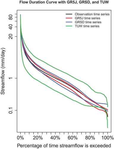
Figure 8 shows the flow-duration curves (FDCs) computed with the observed streamflow and simulations from GR5J, GRSD, and TUW on the reference period, for the 10th and 90th percentiles of the simulation ensembles for each model. While GR5J and GRSD show simulated values close to the observations across the whole regime, TUW exhibits larger ranges around the observations. These contrasted performances shown across the three hydrological models explain the large contribution of hydrological models to the total uncertainty for low-flow projections. For low flows, GR5J computes the narrowest range of values, close to the observations, while TUW shows a larger range of values that tends to overestimate both high and low flows. This can also explain why GR5J simulates low-flow projection values below the average whereas TUW projects low-flow values above the average compared to the mean of the three models (see Fig. 7(i)). Furthermore, the structure of TUW may be less well adapted to model summer low flows in a Mediterranean context (characterized by dry summers) compared to the GR models, since it was developed to represent hydrological regimes of mountainous catchments (Parajka et al. 2016), which are strongly influenced by snowmelt in spring as well as summer and show low flows mainly in winter. To better understand the contribution of the TUW model to the total uncertainty of low-flow projections, the TUW model was excluded from the uncertainty analysis (not shown). The results showed a decrease in the HM contribution from 29% to 15%, by 2085.

Figure 8. Comparison of flow-duration curves on a logarithmic scale for observations and simulations of the reference period (1976–2005), for the 10^th and 90^th percentiles of the simulation ensembles

In this study, only one objective function and the same defined calibration strategies were kept consistent across the three models to investigate the uncertainty related to the HM structure and parameters. Thus, the influence of the objective function selection on the total uncertainty in an impact modelling chain could also be investigated in future work. To improve the quantification and comprehension of the impact of hydrological parameter sets on the total uncertainty, it could be interesting to identify which calibration period and objective function are better suited for hydrological projection according to each HM used. Indeed, the highly contrasted calibration time periods influenced the parameter values selected in the 29 calibration processes. The importance of parameter sets is not the same from one HM to another. Our conclusions regarding the calibration time period of parameter sets as a source of uncertainty depend on the particular hydrological models used in this study. The high contribution of hydrological parametrization to total uncertainty in low-flow projections (in contrast to its 5% contribution to high-flow projections) is supported by Her et al. (2019), who found that uncertainty related to hydrological parametrization was more significant for slow processes.

Finally, low-flow projections show a low sensitivity to future temperature and PET changes, although these are known to be the main drivers of low-flow generation. Rather, low flows seem to follow the precipitation anomaly, inducing a slow decrease and a large associated uncertainty range (Figs 3(d) and 4(a)). This can be explained by the significant uncertainty related to the hydrological models, likely due to a poor representation of slow processes in the models. It could also be explained by the specific geological context and physical properties of the Hérault River catchment that constrain the catchment responses to meteorological drivers. Indeed, upstream of the Gignac gauging station, the hydrological network is largely coupled to a karstic system, which sustains streamflows of the Hérault River, and particularly low-flow levels during the dry season when the temperature is at its highest.

4.2 Other contributions to the total uncertainty

Hydrological model structure and parametrization are not the only things that contribute to the total uncertainty of hydrological projections. The influence of RCPs has a drastic impact on future temperature changes (Christensen and Kjellström 2020). In this study RCPs have an important impact on high-flow projections, but the precipitation projections (Fig. 5) do not depict this contribution from RCPs, so it could be useful to study the precipitation values that are exceeded 5% of the time to complete the study of high-flow drivers. This point could also help the reader to better understand the link between Figs 6 and 7. Indeed, the comparison of autumn precipitation (Fig. 6(d,e,f)) and high-flow (Fig. 7(a,b,c)), confidence bounds is smaller on Fig. 7 than on Fig. 6 and not overlapping. As mentioned, seasonal precipitation analyses could be completed by analysing precipitation values that are exceeded 5% of the time. Moreover, the physics of the catchment constrains the hydrological response, and this is reflected in the HMs. Finally, precipitation is not the only data input for HMs; PET estimation also matters. Kay and Davies (2008) demonstrated the role of PET estimation high-flow projections under climate change study.

As shown in this study, the GCM and RCM uncertainties are major contributors to the uncertainty of low- and high-flow projected changes. Past studies on regional simulations in Europe (e.g. Jacob et al. 2014) show that GCMs exhibit very different seasonal precipitation responses to the forcings, and RCMs add an additional layer of variability in specific regions, typically along the coasts, such as the South-East of France. A larger ensemble, using at best the numerous experiments made recently available in EURO-CORDEX, could improve the estimation of the contributions of these different models to total uncertainty. Up to nine GCMs and 13 RCMs could be accounted for in such an estimate. The total uncertainty may be larger than that estimated here, and the relative contributions of the different type models may prove to be rather modified. One limitation on such work is the ADAMONT downscaling approach used to produce ad hoc weather scenarios for the catchment, which is rather computationally demanding. The direct development of weather scenarios from RCM outputs would be worth considering as it could in practice allow considering the whole body of EURO-CORDEX experiments.

Note also that the residual variance here makes a rather small but non-negligible contribution to the total uncertainty, and is mostly related to the parameter uncertainty of the ANOVA decomposition, as can be seen with the last uncertainty bounds around the estimated main effects (see Figs 6 and 7). In other words, this uncertainty, related to the estimation of the ANOVA parameters, is due to the limited information provided by the outputs of the different modelling chains. Considering a larger ensemble of GCM/RCM couples would likely have, as a side effect, a reduction of this uncertainty component. Finally, it is important to note that the downscaling step was not taken into account in this study and should be considered in future work as it may contribute to the total uncertainty.

4.3 Limitations related to data

Another limitation of this study comes from the available GCM/RCM couples for the downscaling step. This climate impact study was conducted with a small subset of climate projections from EURO-CORDEX downscaled with ADAMONT. The trend and variance of precipitation projections used for this study are shown in Fig. 3. Large uncertainty bounds are related to summer precipitation projections. This is a conflicting message for hydrological models, and this point can explain part of the uncertainty related to low-flow projections. In comparison, the message for autumn precipitation projections is clearer, with a smaller uncertainty range, which leads to a convergent trend for high flows. However, this subset might not be representative of the full EURO-CORDEX projection ensemble: it is part of the wettest projections of EURO-CORDEX (see Ouzeau et al. 2014).

The internal variability was assessed in this study with only one run per modelling chain (only one run is available for each GCM). As shown by Hingray et al. (2019), the larger the number of runs available for a given modelling chain, the better the estimation of the climate response and internal variability of that chain and the better the estimation of all scenario/model uncertainty components of the ensemble of projections. However, ensembles with multiple runs for all modelling chains are not frequent. As mentioned previously, QUALYPSO can be applied even when only one run per modelling chain is available, thanks to the time series approach.

Furthermore, all the climatic projections were downscaled with the same method, ADAMONT. This new downscaling method takes into account the topography, which for the Hérault River catchment is important since it allows representing local extreme Mediterranean events. However, the downscaling method is another step in the impact modelling chain and also contributes uncertainty to the final hydrological projections (Hingray and Saïd 2014, Lafaysse et al. 2014). For future work, it is thus recommended to use at least one more downscaling method to quantify the uncertainty related to the downscaling model in QUALYPSO. For these reasons, the results and interpretations of this study are constrained by the choice of hydrologic and climate models, and are relative to the local case study context, the Hérault River catchment.

Finally, the QE-ANOVA method presents some limits for the study of hydrological extremes under climate change, with the hypotheses not verified as the normal distribution and the homoscedasticity of residuals. This issue comes from the variable studied, a relative anomaly, on hydrological extremes. To improve this particular point, it could be appropriate to evaluate the impact of climate change with absolute anomalies (and not relative anomalies), using data related to other scenarios, to obtain various trends in precipitation projections and approach a more normal distribution of hydrological indicators.

4.4 Contributions and comparison to previous work

This study brings new insights compared to previous hydro-climatic projections on the Hérault River catchment, produced e.g. by Explore 2070 (Chauveau et al. 2013). This project showed different results: for high flows (Q95), the relative change in the future (2046–2065) was estimated to decrease by 7% (min −38% to max +11%). In our study the trend is different, and the new projections show an increase in the mean trend of high-flow indicators, with an increase of 16% by 2060 (from −5% to 35%). For low flows, Explore 2070 showed changes of only −1% to −3% for a low-flow indicator different to MAM7 (the lower 10th percentile, Q10). The main differences come from the methodology: Explore 2070 did not use RCPs, but rather Special report on emissions scenarios (SRES) (from the IPCC assessment report 4 [AR4] report), with a different downscaling method than ADAMONT, and the hydrological model used for the Hérault River catchment was a physically based model, SAFRAN-interface sol biosphère atmosphère (ISBA)-modèle couplé (MODCOU) (Habets et al. 2008). Our results provide an insight into the importance of HMs for the total uncertainty, especially for low-flow projections. Similar results were obtained from other uncertainty analyses, by Bastola et al. (2011), Bosshard et al. (2013), Vidal et al. (2016), and more recently Troin et al. (2018). This result seems to be robust as it does not appear to depend on the estimation method considered. Bosshard et al. (2013), for instance, disregarded internal variability in their ANOVA, which is likely to impact all uncertainty estimates. The estimation of Bastola et al. (2011) was obtained with a rather empirical approach combining generalized likelihood uncertainty estimation (GLUE) and Bayesian model averaging (BMA) methods.

Vidal et al. (2016) used QE-ANOVA on the Durance River catchment, to study uncertainties in low-flow projections. They found a large contribution to the total uncertainty coming from the internal variability and from HM uncertainty. Regarding the uncertainty related to hydrological models, they only considered the model structure component, using different conceptual and physically based hydrological models.

Our results reveal the large contribution that the parametrization of hydrological models can make to the total uncertainty. This conclusion is explained by the choice of hydrological model structure and the number of parameters. The importance of calibrated parameters over different periods for the total uncertainty increases over time. This highlights the fact that much greater attention should be systematically paid to this model calibration issue. Moreover, regarding uncertainty analysis and hydrological response to climatic inputs for low flows, the two studies show different outputs: the Hérault River catchment seems less sensitive than the Durance River catchment to climate change impact regarding temperature changes. In other words, an increase in temperature in an upstream Mediterranean catchment that is partially karstic does not have the same consequences as a similar increase in an Alpine catchment. Our study highlights the regional differences in climate impact studies due to the different hydrological processes that control catchment dynamics, which demonstrates the need to conduct local impact studies.

4.5 Designing adaptation strategies

High- and low-flow periods are key moments for decision makers in terms of water management. To build efficient adaptation strategies to future low flows, assessing future river discharge is essential. This allows the re-evaluation of drought risk and the ability of water resources to satisfy the ecological, domestic, and agricultural water demands (Collet et al. 2015). Figure 9 shows the percentage of ensemble members who agree on different levels of change (from −30 to +60%) for low (Fig. 9(a)) and high flow (Fig. 9(b)) anomalies. The proportion of projections indicating a precise change in anomaly could inform decision makers regarding a date or lead time by which adaption is required.

Figure 9. Proportion of projections showing an anomaly, for (a) low-flow and (b) high-flow projections

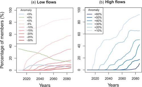
Figure 9(a) shows that, despite the uncertainty associated with low-flow projections with some projections (less than 10% of the ensemble) leading to an increase in low flows of up to +5% in the short lead time, the number of members exhibiting a decrease in low flows, i.e. an intensification of drought hazard, increases with time. By 2050, about 40% of projections converge to a decrease in low flows of at least 5%, and by 2085 more than 50% of low-flow projections agree on this change. Similarly, by 2050, 20% of the ensemble agrees on a decrease in low flows by at least 10%, and 10% of the ensemble converges to a 15% decrease. Stronger decreases also emerge at the long lead time, with about 10% of the projections showing a 20% decrease and 5% of the projections showing a 30% decrease by 2085. This shows that drought hazard is likely to intensify in the future as a result of climate change. Collet et al. (2015) evaluated the feasibility of adaptation strategies in the Hérault River catchment to droughts and showed that even important water consumption reduction strategies (reduction by half for the domestic and irrigation sectors) cannot protect the good ecological state of rivers.

Regarding flood hazard adaptation strategies, the ensemble members converge more clearly for future high-flow anomalies (Fig. 9(b)). By 2050, more than 50% of the ensemble shows a 10% increase of high flows, and 90% of the projections show this by 2085. At the long lead time, more than 60% of projections indicate an increase of more than 20% for high flows, and more than 40% of projections agree on a 40% increase, while 10% of the ensemble agrees on a 60% increase. This shows that flood hazard is very likely to intensify from the middle to the end of the 21st century. This is a strong message to foster further studies to build adaptation strategies in a non-stationary context, and to assess vulnerability and resilience to increasing flood hazard, while making sure the strategies are sustainable for both society and the environment.

5 Conclusion

This work described the methodology and results of new hydrological extreme projections of a Mediterranean catchment (the Hérault River catchment). The approach used in this study was built to analyse the uncertainties related to the different steps of an impact modelling chain with the QUALYPSO method. QUALYPSO proved to be an efficient and robust tool for uncertainty quantification, partitioning, and ranking in a multi-model and multi-scenario framework. Outputs allowed the quantification of transient changes in both high and low flows with the associated uncertainty bounds, but most importantly showed which uncertainty sources contribute the most or least to the total projection ensemble at each time step. Results showed an increase in high flows of 30% to the end of the 21st century, which could result in an increase in flood hazards. For low flows, no clear trend was drawn, since a mean change of −6.5% with large confidence intervals (+12% to −24%) was found. For high flows, internal variability and GCMs/RCMs contribute the most to uncertainty at the short lead time, while RCPs provide the largest uncertainty contribution by 2085. The ranking of uncertainty sources is different for low flows, where HMs and hydrological model parameters contribute the greatest uncertainty.

This last point raises the importance of estimating hydrological structure and parameter uncertainty. In other words, evaluation of the calibration approaches and model robustness cannot be overlooked by hydrological modellers in climate impact studies, since appropriate expertise could help reduce the projection uncertainty range. The residual variance of the impact modelling chain could be reduced by using a higher number of GCM/RCM couples that complete the GCM/RCM matrix. Moreover, another set of GCM/RCM couples that cover a larger spectrum of possible futures in terms of precipitation change could also give more representative low-flow projections.

These results are specific to the Hérault River catchment and can be useful to local stakeholders to implement strategies for adaptation to hydrological extremes, particularly for high flows. This approach is a first step to a climate impact study on water resources at the catchment scale, and could provide a solid basis on which to build future adaptation strategies. To evaluate the impact on vulnerability, it is necessary to integrate into the existing modelling chain water demand models, and take into account the uncertainty related to these added models.

Finally, the QE-ANOVA method is not free of limitations. For example, concerning the study of hydrological extremes under climate change, two critical assumptions are that residuals are assumed to follow a Gaussian distribution and to be homoscedastic. These assumptions may be not verified for some climate variables, such as hydrological extremes, which are likely to be skewed or bounded (e.g. low flows). The possibility to adapt the ANOVA framework to such configurations would be worth investigating in future work.

Acknowledgements

The authors thank Météo-France and SCHAPI for providing climatic and streamflow data, respectively.

Disclosure statement

No potential conflict of interest was reported by the authors.

References

- Addor, N., et al., 2014. Robust changes and sources of uncertainty in the projected hydrological regimes of Swiss catchments. Water Resources Research, 50 (10), 7541–7562. doi:https://doi.org/10.1002/2014WR015549.
- Bastola, S., Murphy, C., and Sweeney, J., 2011. The role of hydrological modelling uncertainties in climate change impact assessments of Irish river catchments. Advances in Water Resources, 34 (5), 562–576. doi:https://doi.org/10.1016/j.advwatres.2011.01.008.
- Bauwens, A., Sohier, C., and Degré, A., 2011. Hydrological response to climate change in the Lesse and the Vesdre catchments: contribution of a physically based model (Wallonia, Belgium). Hydrology and Earth System Sciences, 15 (6), 1745–1756. doi:https://doi.org/10.5194/hess-15-1745-2011.
- Blöschl, G., et al., 2019. Twenty-three unsolved problems in hydrology (UPH) – a community perspective. Hydrological Sciences Journal, 64 (10), 1141–1158. doi:https://doi.org/10.1080/02626667.2019.1620507.
- Bosshard, T., et al., 2013. Quantifying uncertainty sources in an ensemble of hydrological climate-impact projections: uncertainty sources in climate-impact projections. Water Resources Research, 49 (3), 1523–1536. doi:https://doi.org/10.1029/2011WR011533.
- CGDD, 2019. L’évaluation socioéconomique des projets de prévention des inondations en France. https://www.ecologique-solidaire.gouv.fr/levaluation-economique-des-projets-gestion-des-risques-naturels.
- Chauveau, M., et al., 2013. Quels impacts des changements climatiques sur les eaux de surface en France à l’horizon 2070 ? La Houille Blanche. 4, 5–15. doi:https://doi.org/10.1051/lhb/2013027
- Christensen, O.B. and Kjellström, E., 2020. Partitioning uncertainty components of mean climate and climate change in a large ensemble of European regional climate model projections. Climate Dynamics, 54 (9–10), 4293–4308. doi:https://doi.org/10.1007/s00382-020-05229-y.
- Collet, L., et al., 2015. Water supply sustainability and adaptation strategies under anthropogenic and climatic changes of a meso-scale Mediterranean catchment. Science of the Total Environment, 536, 589–602. doi:https://doi.org/10.1016/j.scitotenv.2015.07.093
- Collet, L., Beevers, L., and Prudhomme, C., 2017. Assessing the impact of climate change and extreme value uncertainty to extreme flows across Great Britain. Water, 9 (2), 103. doi:https://doi.org/10.3390/w9020103.
- Coron, L., et al., 2017. The suite of Lumped GR hydrological models in an R package. Environmental Modelling and Software, 94, 166–171. doi:https://doi.org/10.1016/j.envsoft.2017.05.002.
- Coron, L., et al., 2019. airGR: suite of GR hydrological models for precipitation-runoff modelling. R package version 1.3.2.42. Available from: https://CRAN.R-project.org/package=airGR [Accessed 24 March 2021].
- De Lavenne, A., et al., 2019. A regularization approach to improve the sequential calibration of a semi‐distributed hydrological model. Water Resources Research, 55 (11), 8821–8839. doi:https://doi.org/10.1029/2018WR024266.
- Delaigue, O., et al., 2019. Base de données hydroclimatique à l’échelle de la France. IRSTEA, UR HYCAR, Équipe Hydrologie des bassins versants, Antony. Available from: https://webgr.inrae.fr/base-de-donnees/ [Accessed 24 March 2021].
- Déqué, M., et al., 2007. An intercomparison of regional climate simulations for Europe: assessing uncertainties in model projections. Climatic Change, 81 (S1), 53–70. doi:https://doi.org/10.1007/s10584-006-9228-x.
- Déqué, M., et al., 2012. The spread amongst ENSEMBLES regional scenarios: regional climate models, driving general circulation models and interannual variability. Climate Dynamics, 38 (5–6), 951–964. doi:https://doi.org/10.1007/s00382-011-1053-x.
- Diffenbaugh, N.S. and Giorgi, F., 2012. Climate change hotspots in the CMIP5 global climate model ensemble. Climatic Change, 114 (3–4), 813–822. doi:https://doi.org/10.1007/s10584-012-0570-x.
- Dobler, C., et al., 2012. Quantifying different sources of uncertainty in hydrological projections in an Alpine watershed. Hydrology and Earth System Sciences, 16 (11), 4343–4360. doi:https://doi.org/10.5194/hess-16-4343-2012.
- Dorchies, D., et al., 2014. Climate change impacts on multi-objective reservoir management: case study on the Seine River basin, France. International Journal of River Basin Management, 1–19. doi:https://doi.org/10.1080/15715124.2013.865636
- Edenhofer, O., et al., 2011. Renewable energy sources and climate change mitigation: special report of the intergovernmental panel on climate change. Cambridge: Cambridge University Press.
- Evin, G., et al., 2019. Partitioning uncertainty components of an incomplete ensemble of climate projections using data augmentation. Journal of Climate, 32 (8), 18. doi:https://doi.org/10.1175/JCLI-D-18-0606.1.
- Evin, G., 2019. QUALYPSO: partitioning uncertainty components of an incomplete ensemble of climate projections. R package version 1.1. Available from: https://CRAN.R-project.org/package=QUALYPSO [Accessed 24 March 2021].
- Fabre, J., et al., 2016. Reducing the gap between water demand and availability under climate and water use changes: assessing the effectiveness and robustness of adaptation. La Houille Blanche. 6, 21–29. doi:https://doi.org/10.1051/lhb/2016056
- Field, C.B., et al., eds., 2014. Freshwater resources. In: Climate change 2014 impacts, adaptation, and vulnerability. Cambridge: Cambridge University Press, 229–270. https://doi.org/10.1017/CBO9781107415379.008
- Grouillet, B., et al., 2016. Sensitivity analysis of runoff modeling to statistical downscaling models in the western Mediterranean. Hydrology and Earth System Sciences, 20 (3), 1031–1047. doi:https://doi.org/10.5194/hess-20-1031-2016.
- Guiot, J. and Cramer, W., 2016. Conclusion. Le bassin méditerranéen, le changement climatique et notre avenir commun: lancer de nouvelles initiatives de recherche pour guider les décisions politiques futures. In: J. Moatti and S. Thiébault, eds. The Mediterranean region under climate change: a scientific update. Marseille: IRD Éditions, 665–669. doi:https://doi.org/10.4000/books.irdeditions.24066.
- Gupta, H.V., et al., 2009. Decomposition of the mean squared error and NSE performance criteria: implications for improving hydrological modelling. Journal of Hydrology, 377 (1–2), 80–91. doi:https://doi.org/10.1016/j.jhydrol.2009.08.003.
- Habets, F., et al., 2008. The SAFRAN‐ISBA‐MODCOU hydrometeorological model applied over France. J. Geophys. Res, 113, D06113. doi:https://doi.org/10.1029/2007JD008548.
- Haddeland, I., et al., 2014. Global water resources affected by human interventions and climate change. Proceedings of the National Academy of Sciences, 111 (9), 3251–3256. doi:https://doi.org/10.1073/pnas.1222475110.
- Hattermann, F.F., et al., 2017. Cross‐scale intercomparison of climate change impacts simulated by regional and global hydrological models in eleven large river basins. Climatic Change, 141 (3), 561–576. doi:https://doi.org/10.1007/s10584-016-1829-4.
- Hawkins, E. and Sutton, R., 2009. The potential to narrow uncertainty in regional climate predictions. Bulletin of the American Meteorological Society, 90 (8), 1095–1108. doi:https://doi.org/10.1175/2009BAMS2607.1.
- Hawkins, E. and Sutton, R., 2011. The potential to narrow uncertainty in projections of regional precipitation change. Climate Dynamics, 37 (1–2), 407–418. doi:https://doi.org/10.1007/s00382-010-0810-6.
- Her, Y., et al., 2019. Uncertainty in hydrological analysis of climate change: multi-parameter vs. multi-GCM ensemble predictions. Scientific Reports, 9, 4974. doi:https://doi.org/10.1038/s41598-019-41334–7.
- Hertig, E. and Tramblay, Y., 2017. Regional downscaling of Mediterranean droughts under past and future climatic conditions. Global and Planetary Change, Elsevier, 151, 36–48. doi:https://doi.org/10.1016/j.gloplacha.2016.10.015
- Hingray, B., et al., 2019. Uncertainty component estimates in transient climate projections: precision of estimators in a single time or time series approach. Climate Dynamics, 53 (5–6), 2501–2516. doi:https://doi.org/10.1007/s00382-019-04635-1.
- Hingray, B. and Saïd, M., 2014. Partitioning Internal variability and model uncertainty components in a multimember multimodel ensemble of climate projections. Journal of Climate, 27 (17), 6779–6798. doi:https://doi.org/10.1175/JCLI-D-13-00629.1.
- International Environmental Modelling and Software Society (iEMSs), 2012. International congress on environmental modelling and software managing resources of a limited planet. In: Sixth Biennial Meeting, Leipzig, Germany.
- Jacob, D., et al., 2014. EURO-CORDEX: new high-resolution climate change projections for European impact research. Regional Environmental Change, 14 (2), 563. doi:https://doi.org/10.1007/s10113-013-0499-2.
- Kay, A.L., et al., 2009. Comparison of uncertainty sources for climate change impacts: flood frequency in England. Climatic Change, 92 (1–2), 41–63. doi:https://doi.org/10.1007/s10584-008-9471-4.
- Kay, A.L. and Davies, H.N., 2008. Calculating potential evaporation from climate model data: a source of uncertainty for hydrological climate change impacts. Journal of Hydrology, 358 (3–4), 221–239. doi:https://doi.org/10.1016/j.jhydrol.2008.06.005.
- Kundzewicz, Z.W., et al., 2008. The implications of projected climate change for freshwater resources and their management. Hydrological Sciences Journal, 53 (1), 3–10. doi:https://doi.org/10.1623/hysj.53.1.3.
- Lafaysse, M., et al., 2014. Internal variability and model uncertainty components in future hydrometeorological projections: the Alpine Durance basin. Water Resources Research, 50 (4), 3317–3341. doi:https://doi.org/10.1002/2013WR014897.
- Leleu, I., et al., 2014. La refonte du système d’information national pour la gestion et la mise à disposition des données hydrométriques. La Houille Blanche, (1), 25–32. doi:https://doi.org/10.1051/lhb/2014004.
- Lespinas, F., Ludwig, W., and Heussner, S., 2014. Hydrological and climatic uncertainties associated with modeling the impact of climate change on water resources of small Mediterranean coastal rivers. Journal of Hydrology, 511, 403–422. doi:https://doi.org/10.1016/j.jhydrol.2014.01.033
- Marcos-Garcia, P., Lopez-Nicolas, A., and Pulido-Velazquez, M., 2017. Combined use of relative drought indices to analyze climate change impact on meteorological and hydrological droughts in a Mediterranean basin. Journal of Hydrology, 554, 292–305. doi:https://doi.org/10.1016/j.jhydrol.2017.09.028
- Marx, A., et al., 2018. Climate change alters low flows in Europe under global warming of 1.5, 2, and 3°C. Hydrology and Earth System Sciences, 22 (2), 1017–1032. doi:https://doi.org/10.5194/hess-22-1017-2018.
- Milano, M., et al., 2012. Facing climatic and anthropogenic changes in the Mediterranean basin: what will be the medium-term impact on water stress? Comptes Rendus Geoscience, 344 (9), 432–440. doi:https://doi.org/10.1016/j.crte.2012.07.006.
- Milano, M., et al., 2013. Current state of Mediterranean water resources and future trends under climatic and anthropogenic changes. Hydrological Sciences Journal, 58 (3), 498–518. doi:https://doi.org/10.1080/02626667.2013.774458.
- Mitchell, T.D. and Hulme, M., 1999. Predicting regional climate change: living with uncertainty. Progress in Physical Geography: Earth and Environment, 23 (1), 57–78. doi:https://doi.org/10.1177/030913339902300103.
- Monteith, J.L., 1965. Evaporation and environment. Symposia of the Society for Experimental Biology, 19, 205–234.
- Ouzeau, G., et al., 2014. Le climat de la France au XXIe siècle : rapports remis à Ségolène Royal. Paris: Ministre de l’écologie, du développement durable et de l’énergie, le 6 septembre 2014.
- Parajka, J., et al., 2016. Uncertainty contributions to low-flow projections in Austria. Hydrology and Earth System Sciences, 20 (5), 2085–2101. doi:https://doi.org/10.5194/hess-20-2085-2016.
- Parajka, J., Merz, R., and Blöschl, G., 2007. Uncertainty and multiple objective calibration in regional water balance modelling: case study in 320 Austrian catchments. Hydrological Processes, 21 (4), 435–446. doi:https://doi.org/10.1002/hyp.6253.
- Piras, M., et al., 2014. Quantification of hydrologic impacts of climate change in a Mediterranean basin in Sardinia, Italy, through high-resolution simulations. Hydrology and Earth System Sciences, 18 (12), 5201–5217. doi:https://doi.org/10.5194/hess-18-5201-2014.
- Post, J., et al., 2012. Quantifying and reducing uncertainty in the assessment of water-related risks in southern Europe and neighbouring countries. 9.
- Pushpalatha, R., et al., 2011. A downward structural sensitivity analysis of hydrological models to improve low-flow simulation. Journal of Hydrology, 411 (1–2), 66–76. doi:https://doi.org/10.1016/j.jhydrol.2011.09.034.
- Refsgaard, J.C., et al., 2013. The role of uncertainty in climate change adaptation strategies—a Danish water management example. Mitigation and Adaptation Strategies for Global Change, 18 (3), 337–359. doi:https://doi.org/10.1007/s11027-012-9366-6.
- Sauquet, E., et al., 2016. Le partage de la ressource en eau sur la Durance en 2050: vers une évolution du mode de gestion des grands ouvrages duranciens? La Houille Blanche, 5 (5), 25–31. doi:https://doi.org/10.1051/lhb/2016046.
- Schewe, J., et al., 2014. Multimodel assessment of water scarcity under climate change. Proceedings of the National Academy of Sciences, 111 (9), 3245–3250. doi:https://doi.org/10.1073/pnas.1222460110.
- Sellami, H., et al., 2016. Quantifying hydrological responses of small Mediterranean catchments under climate change projections. Science of the Total Environment, 543, 924–936. doi:https://doi.org/10.1016/j.scitotenv.2015.07.006
- Sénat, 2019. Adapter la France aux dérèglements climatiques à l’horizon 2050: urgence déclarée. Available from: http://www.senat.fr/rap/r18-511/r18-511.html [Accessed 24 March 2021].
- Thiébault, S. and Moatti, J.-P., 2018. Introduction. Le changement climatique en Méditerranée. Abridged English/French version. Marseille: IRD Éditions.
- Thirel, G., et al., 2019. Quels futurs possibles pour les débits des affluents français du Rhin (Moselle, Sarre, Ill)? La Houille Blanche, 5 (5–6), 140–149. doi:https://doi.org/10.1051/lhb/2019039.
- Thirel, G., Andréassian, V., and Perrin, C., 2015. On the need to test hydrological models under changing conditions. Hydrological Sciences Journal, 60 (7–8), 1165–1173. doi:https://doi.org/10.1080/02626667.2015.1050027.
- Tramblay, Y. and Somot, S., 2018. Future evolution of extreme precipitation in the Mediterranean. Climatic Change, 151 (2), 289–302. ISSN 0165-0009. doi:https://doi.org/10.1007/s10584-018-2300-5.
- Troin, M., et al., 2018. Uncertainty of hydrological model components in climate change studies over two nordic quebec catchments. Journal of Hydrometeorology, 19 (1), 27–46. doi:https://doi.org/10.1175/JHM-D-17-0002.1.
- Verfaillie, D., et al., 2017. The method ADAMONT v1.0 for statistical adjustment of climate projections applicable to energy balance land surface models. Geoscientific Model Development, 10 (11), 4257–4283. doi:https://doi.org/10.5194/gmd-10-4257-2017.
- Vidal, J.-P., et al., 2010. A 50-year high-resolution atmospheric reanalysis over France with the Safran system. International Journal of Climatology, 30 (11), 1627–1644. doi:https://doi.org/10.1002/joc.2003.
- Vidal, J.-P., et al., 2016. Hierarchy of climate and hydrological uncertainties in transient low-flow projections. Hydrology and Earth System Sciences, 20 (9), 3651–3672. doi:https://doi.org/10.5194/hess-20-3651-2016.
- Viglione, A. and Parajka, J., 2019. TUWmodel: lumped/semi-distributed hydrological model for education purposes. R package version 1.0-2. Available from: https://CRAN.R-project.org/package=TUWmodel [Accessed 24 March 2021].
- Yip, S., et al., 2011. A simple, coherent framework for partitioning uncertainty in climate predictions. Journal of Climate, 24 (17), 4634–4643. doi:https://doi.org/10.1175/2011JCLI4085.1.