Assessment of drainage network analysis methods to rank sediment yield hotspots

ABSTRACT

This paper aims to test different methods used for assessing sediment yield indices to identify hotspots and rank sediment yield hotspots. This process includes the assessment of the entropy weighting (EW), fractal dimension (FD), slope length gradient (SL), and sediment connectivity (SC) methods. The indices at different sub-catchment levels were applied in the Ilanlu catchment (Iran) and organized based on five sediment hazard classes. To assess the performance of sediment hazard mapping, a method of superimposition was used and assessed with the erosion potential model (EPM). The superimposition showed that 8, 10, 4 and 9 sub-catchments, based on the degree of susceptibility, obtained the highest results from FD, EW, SL and SC, respectively, compared with the EPM model. The results show that EW and SC methods can achieve greater performance than FD and SL in identifying sediment production hotspots.

KEYWORDS:

• cluster analysis
• sediment yield
• modelling
• soil erosion

Editor A. Fiori Associate Editor M. Nones

1 Introduction

Soil erosion and sediment-related problems are associated with dramatic adverse impacts on the environment and agriculture, including economic loses, water quality, reducing the storage capacity of reservoirs and decreased agricultural production (Alexakis et al. 2013, Nasre et al. 2013, Shit et al. 2015). Due to the huge cost of watershed management actions to reduce the consequences of soil erosion and sediment-related problems (Kiani-Harchegani et al. 2018, Kiani-Harchegani and Sadeghi 2020), areas vulnerable to erosion should be identified to justify and develop sustainable and clean soil and water conservation measures. To this end, many algorithms have been developed to prioritize at the sub-catchment scale based on sediment control measurements, to help manage watersheds easily and cost-effectively (Kouli et al. 2009, Kalantari et al. 2019).

Among catchment geomorphology characteristics, the river network is among the most important in terms of impacts on soil erosion, flood, and sediment yield processes. This is because of its implications for water quality and quantity and potential uses at different scales (Al-Dulaimi and Younes, 2017, García‐Ruiz et al. 2017, Yegemova et al. 2018). Therefore, an accurate description of river network geomorphology is crucial for investigating river flow, sediment transport, and floods (Ariza-Villaverde et al. 2013, Zhang et al. 2015).

The methods of describing river networks have been divided into regular and irregular groups by several researchers. In the former group, only the flow pattern characteristics, such as drainage network length and drainage network gradient, are used to describe the drainage network (Mandelbrot 1967, Snow 1989, Prosser et al. 2001, Snelder and Biggs 2002, Piégay et al. 2005, Zhang et al. 2015). Sediment connectivity (SC) and slope length gradient (SL) are two well-known regular methods employed for the analysis of different soil erosion and sediment dynamics processes (e.g. Marçal et al. 2017, Poeppl et al. 2019, Turnbull and Wainwright 2019, Najafi et al. 2020).

Llena et al. (2019) used the SC method to assess the effects of decadal-scale land-use and topographic changes on the transfer of water and sediment through coupling relationships among its components. In another application, Troiani and Della Seta (2008) used the SL method as a proxy for stream power to delineate the capacity of the drainage network to transport sediment and erode its bed.

Although the regular methods are widely used, studies by Hassan and Kurths (2002), Zhang et al. (2015), and Malekinezhad et al. (2017) suggest that these methods may not fully represent the current drainage network irregularities, emphasizing the need for alternative analyses. As a result, there is a growing use of other methods, which are relatively newer than the SC and SL, to analyse drainage networks. These methods have been developed based on irregular properties of objects (i.e. drainage networks) and provide more fitting descriptions of these characteristics than regular methods do (Mandelbrot 1967, Snow 1989, Zhang et al. 2015, Sepehri et al. 2018). The fractal dimension (FD) is one of the most popular methods in this category. Recent applications of FD focus not only on geomorphological studies (Nur et al. 2016, Hu et al. 2020) but also on topics such as astronomy (De Cola and Lam 2002, Kusák 2014), geology (Dou et al. 2020, Zhang et al. 2020), meteorology (Zhou et al. 2020, Yao et al. 2020), and hydrology (Zhang et al. 2015, Al-Wagdany et al. 2020).

Entropy weighting (EW) is another method utilized to assess the drainage network irregularity, precipitation, water quality, soil moisture, groundwater networks, and sediment studies (Su and You 2014, Stosic et al. 2017, Keum et al. 2017, Pournader et al. 2018, Arabameri et al. 2019). Depending on what property of the drainage network is considered, EW can be categorized as an irregular method or a regular method. For example, Fiorentino et al. (1993) employed the regular method “entropy of the Horton-Strahler ordering” for drainage network analysis. In contrast, the EW method is classified as an irregular method if it is used to assess drainage network irregularities and relationship with other aspects of studies on natural hazards, such as soil erosion, sediment yields or flood.

To on best our knowledge, on one hand, there is scarce information about applications of EW for assessing the irregularity of drainage networks and its relationship with sediment yield, flood hazard and other natural hazard studies. On the other hand, there are very few studies comparing irregularity and regularity properties of drainage networks related to hydrology studies in developing countries with catchments that register high sedimentation problems. Therefore, to fill this gap, this research aims to compare regular and irregular methods to prioritize sub-catchments by sediment yield. This process includes the assessment of the EW, FD, SL, and SC methods. These indices, at different sub-catchment levels, were first estimated and then organized based on five sediment hazard classes using hierarchical clustering. To assess the performance of sediment hazard mapping, a superimposition method was used, and the modelling results were assessed using the erosion potential model (EPM). To achieve this goal, we selected the Ilanlu catchment in the Northwest Hamadan, Iran.

2 Materials and methods

2.1 Study area

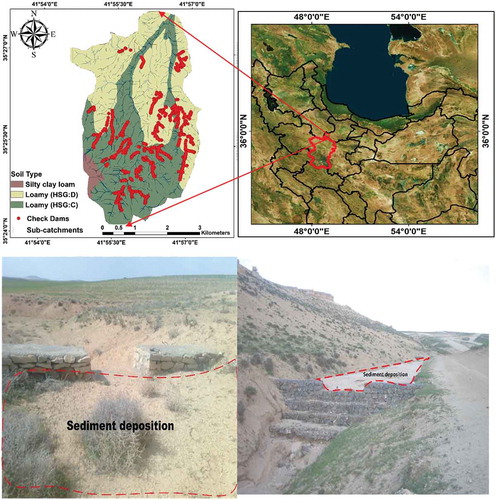
The study site is located in a catchment with an area of 17.89 km² in the northwest of Hamadan Province, Iran. According to data from the Asad-Abad Weather Station (31°24ʹ45″–31°27ʹ 29″N, 41°55ʹ20″–41°57ʹ34″E) collected between 1997 and 2015, near the Ilanlu catchment, the average temperature of the study site is 10.8°C (−15 to +34°C). February and August are the coldest and hottest months, respectively. The annual average precipitation is 443 mm. According to the ombrothermic curve, the driest months of the year are May to September, which corresponds to a semi-arid region. The predominant drainage network pattern is dendritic in some parts of the catchment, and becomes parallel due to the hillslope steepness, which is characterized by the presence of lime covered by a clay layer (Fig. 1). In the upstream catchment sections, a small portion of precipitation reaches the lower layers. This amount of water flows from springs, and the remaining portion of the rainfall runs off over the catchment where the permeable lithic-rich facies intersect non-permeable sediments (Ildoromi et al. 2019).

Figure 1. Location of the Ilanlu catchment in Hamadan Province and Iran and examples of check dams with collecting sediments

2.2 Methodology

This section briefly explains the drainage network assessment methods under investigation. These methods reveal irregularities of drainage networks and show their relationships with sediment productivity/transport and possible yield.

2.2.1 Regularity methods

2.2.1.1 Stream length gradient (SL)

This method depends strongly on the flow power (Bizzi and Lerner 2015, Troiani et al. 2017, Moussi et al. 2018). In a specific reach of a drainage network, the stream power is a measure of hydraulic driving forces associated with sediment detachment and transport processes (Burbank and Anderson 2001, Troiani and Della Seta 2008). Troiani et al. (2017) and Yang et al. (2019) used the SL method to define a measure of river flow power in a unit of length. They also used this method to define a portion of the river flow energy at a certain reach of the river and relate it to the capability of a stream to transport sediments and to erode its bed (Table 1).

Table 1. Summary and examples of the different regular and irregular equations used in Ilanlu catchment

Descriptor	Equation	Reference
Fractal dimension	$d=\frac{log\left(N\right)}{log\left(r_b\right)}$	Martínez-Mena et al. (1999); Xu et al. (2014); De Freitas Sampaio et al. (2019)
Entropy weighting	$p_i=-k\sum _{j=1}^n{f}_{ij}ln{f}_{ij}$$f_{ij}=\frac{r_{ij}}{\sum _{j=1}^n{r}_{ij}},k=1/lnn$$r_{ij}=\frac{x_{ij}-min{\left\{x_{ij}\right\}}_i}{max{\left\{x_{ij}\right\}}_i-min{\left\{x_{ij}\right\}}_i}$${\lambda }_i=\frac{1-p_i}{m-\sum _{i=1}^m{p}_i}$	Pournader et al. (2018); Arabameri et al. (2019); Chen et al. (2019)
Sediment connectivity	$SC=lo{g}_{10}\left(\frac{D_{up}}{D_{dn}}\right)$$D_{up}=\bar{W}\bar{S}\sqrt{A}$$D_{dn}=\hspace{0.17em}\sum \frac{d_i}{W_i{S}_i}$$\bar{W}=1-\frac{\left(altitudemean-altitude\right)}{altituderange}$	Sandercock and Hooke (2011); Sougnez et al. (2011); López-Vicente et al. (2013); Kalantari et al. (2019); Sherriff et al. (2019)
Stream length gradient	$SL=\left(\frac{\mathrm{\Delta }H}{\mathrm{\Delta }L}\right)\times L$	Moussi et al. (2018); Troiani et al. (2017); Hamza et al. (2019)

d: fractal dimension; N: number of measurement scales; r_b: small segments of box-counting method (pixel size) r: length of the phenomenon; r_ij: normalization index; X_ij: number of networks in which the drainage network is available; P_i: entropy value; λ_i: weight of the ith index; SL: stream length gradient; ΔH: maximum and minimum of elevation of a given stream reach; ΔL: total length of the segment; L: distance from the source of the river to a minimum elevation of the segment; SC: sediment connectivity; W: average weighting factor of the upslope contributing area; A: dimensionless and equal to macro roughness; S: average slope gradient of the upslope contributing area (m²); Si: the slope gradient of the i^th cell (m m⁻¹).

2.2.1.2 Sediment connectivity (SC)

The relationship between flow and sediment, as two major attributes of sediment distribution throughout the catchment, reveals the linkage between the sediment site and upstream discharge into the downstream (Sandercock and Hooke 2011, Sougnez et al. 2011, López-Vicente et al. 2013). This is a very popular index among researchers due to its simplicity, minimal information requirement, and complementarity with field observations. According to Sougnez et al. (2011), López-Vicente et al. (2015), Zhang et al. (2017), Mahoney et al. (2018), and Estrany et al. (2019), a high SC value indicates the predominance of erosion over sedimentation, and the desired point typically has a high rate of sediment transportation and sediment continuity (Table 1).

2.2.2 Irregularity methods

2.2.2.1 Fractal dimension (FD). F

ractals are used to describe irregular natural objects. Contrary to the Euclidean method used to describe regular objects (e.g. 0 for point objects and values of 1, 2, and 3 for lines, planes and volume objects, respectively; Chen et al. 2019), fractal theory determines the dimension of irregularity of fractal objects using the property of self-similarity, which can be categorized as 1 < d < 2 and 2 < d < 3 for two-dimensional and three-dimensional spaces, respectively (Table 1). These methods eliminate the barriers of regular ones in one-, two- and three-dimensional spaces. Therefore, the fractal offers a more comprehensive account of the real properties and their irregularity (Zhang et al. 2015, Malekinezhad et al. 2017). Although self-similar structures are not necessarily fractal, fractals typically involve self-similarity (Zhang et al. 2015, Malekinezhad et al. 2017). In the field of hydrology, FD is used to present the drainage network irregularity and its relationship with soil erosion, flooding and sediment yield (Ariza-Villaverde et al. 2013).

2.2.2.2 Entropy weighting (EW)

EW measures the properties of such structures as disorder, instability, and uncertainty. Stephan Boltzmann (1877) proposed this method, and later it was quantitatively described by Shannon (1948). This study uses the EW to assess the change in the self-similar properties of the objects (Jaafari et al. 2014). The FD uses a regression relationship for such assessments (Table 1).

2.2.3 Workflow

Figure 2 presents the workflow used to determine and develop various catchment layers to assess the efficiency of different sediment distribution methods across the catchment. To this end, the catchment under investigation was assessed using ArcHydro (as an add-in to the ArcGIS 10.7 software) and the automatic catchment delineation tools, which divided the watershed into 28 sub-catchments using the topographic map (scale 1:50 000 and contour interval 20 m).

Figure 2. Flowchart of the proposed methods

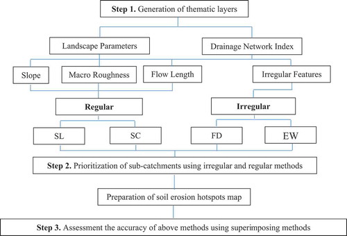
Further, the drainage networks of the sub-catchments were regarded as input data for FD and EW, to assess their irregularity and to establish their linkage to the degree of sediment transportation. The SL and SC methods require more than drainage data, including macro-roughness and slope layer data obtained from applying Digital elevation model (DEM) to the catchment (Fig. 2). After collecting the required data and measuring the susceptibility of sub-catchments to sediment yield using the aforementioned methods and the EPM method, hierarchical cluster analysis (HCA) was used to divide the total area into five classes, namely very high, high, moderate, low, and very low sediment yield susceptibility.

2.2.4 Clustering algorithm to apply SL and SC methods

The FD and EW methods produce only one value of the sediment yield index for each sub-catchment, whereas the SL and SC methods produce a series of SL and SC index values for every sub-catchment across the river network. In this regard, to assign a single SL and SC index value to each sub-catchment, it is necessary to transform the series values to a raster map based on an interpolation method. In this study, inverse distance weighting (IDW) interpolation was used to produce the raster map of the SL/SC index. Then, the blow algorithm was applied to assign a single value related to the SL/SC index for each sub-catchment:

• Step 1: Reclassify each sub-catchment into one of five classes based on its SL or SC index value.

• Step 2: Assign specific values (w_ij) to each class using analytic hierarchy process (AHP; Table 2) and then assign values for H_i to each sub-catchment using Equation (1):

(1) $H_{i=1:28}=\sum _{j=1}^5{w}_{ij}.x_{ij}$(1)

Table 2. Assigned weights for the classes of the SL and SC methods

	Primary score					Weighting
	Very high	High	Moderate	Low	Very low
Very high	1	4	5	7	8	0.52
High	…	1	4	5	6	0.25
Moderate	…	…	1	4	5	0.13
Low	…	…	…	1	2	0.05
Very low	…	…	…	…	1	0.04

where X_ij is the percentage of areas under different classes of SL or SC (Stage 1), i represents the number of sub-catchments, and j denotes the class of SL and SC values (e.g. j = 1 is for very low SL and SC and j = 5 is for very high SL and SC).

• Step 3: Cluster all sub-catchments into five clusters, considering the sediment yield rate, using HCA.

2.3 Hierarchical cluster analysis

After calculating the sediment yield rate for every sub-catchment, HCA was utilized to identify the sub-catchments with similar sediment yield rates. This technique involves three steps (Ouarda et al. 2008):

1. Determine the similarity among sub-catchments using a paired comparison. At this stage, the degree of proximity and similarity is determined using the distance criterion or the difference in the values of the erodibility index between sub-catchments.

2. Classify the sub-catchments in a binary hierarchical tree using a linkage function. Here, in the linkage function, the paired sub-catchments with similar erodibility scores are placed in the same cluster (step 1). In the next step, all clusters are grouped in a larger cluster. This process is continued to form a hierarchical tree.

3. Identification of clusters: during this last step, clusters are grouped in a hierarchical tree and the hierarchical tree is cut at an arbitrary point to distinguish the clusters.

To apply the HCA, two methods, Minkowski distance (Equation (2)(2) $d\left(a,b\right)={\left(\sum _{i=1}^n{\left|ai-bi\right|}^{\lambda }\right)}^{1/\lambda }$(2) ) and Ward’s linkage (Equations (3)(3) $WS{S}_p=\sum _{i=1}^{n_p}{d}^2\left(X_{pi},X_p^{-}\right)$(3) and (4(4) $d\left(p,q\right)=WS{S}_{\left(p+q\right)}-\left(WS{S}_p+WS{S}_q\right)=\frac{n_p{n}_q{d}^2\left(X_p^{-},X_q^{-s}\right)}{n_p+n_q}$(4) ); Lin and Chen 2006, Ouarda et al. 2008), were applied, as distance and linkage functions, respectively. The Minkowski distance is a metric in a normed vector space, used to measure the distance between two variables. Ward’s method is a sum of Euclidean distances between cluster means for all inter-cluster variables, in that each variable is made incremental. Therefore, an increase in the total within-cluster sum of squares (WSS) leads to the combination of two clusters, p and q (Lin and Chen 2006, Ouarda et al. 2008). The WSS is the total distance between inter-cluster objects and the cluster’s centre of gravity (i.e. the mean vector):

(2) $d\left(a,b\right)={\left(\sum _{i=1}^n{\left|ai-bi\right|}^{\lambda }\right)}^{1/\lambda }$(2)

where a_i and b_i are the i^th arguments of the sets (sediment production rate of the sub-catchments); a, b and λ are a parameter such that λ (−∞, ∞), which is assumed to be 3:

(3) $WS{S}_p=\sum _{i=1}^{n_p}{d}^2\left(X_{pi},X_p^{-}\right)$(3)

where n_p and x_p stand, respectively, for the size and the centroid of cluster p. Following this equation, the distance between clusters p and q can be obtained:

(4) $d\left(p,q\right)=WS{S}_{\left(p+q\right)}-\left(WS{S}_p+WS{S}_q\right)=\frac{n_p{n}_q{d}^2\left(X_p^{-},X_q^{-s}\right)}{n_p+n_q}$(4)

2.4 Performance evaluation

Having observed sediment data is a necessary condition for using physically based distributed models to simulate and validate the sediment yield of a basin (Aga et al. 2020). One of the most important challenges, especially in developing countries, is related to the scarcity or unavailability of measured sediment data. Therefore, in recent years various empirical models have been extended to predict sediment yield in the form of either suspended or bed load. The acceptable performance of these models depends largely on how the required data are measured (Ildoromi et al. 2019).

In this study, among the empirical methods, EPM was used to evaluate the consistency of classified outputs of the FD, EW, SC, and SL methods. EPM is a well-known empirical method that has been successfully used in many regions, especially in developing countries where sediment data are scarce (Noori et al. 2016, Najafi et al. 2020). In this study, to estimate the indicators of this method, we used data provided by the Department of Natural Resources of Hamadan Province. These data were collected by experts via regular field measurements and surveys. The majority of the data collection was controlled under field conditions, which would reduce the uncertainty of the accuracies of the outputs.

The EPM model for calculating erosion (Equations (5)(5) $Z=Y.X_a\left(\theta +\sqrt{I}\right)$(5) and (6(6) $Wsp=TH\pi Z^{1.5}$(6) )) and sediment yield (Equations (7)(7) $G_{sp}=Wsp.R_u$(7) and (8(8) $Ru=\frac{4{\left(P\times D\right)}^{0.5}}{L+10}$(8) )) requires six factors, i.e. surface geology, soils, topographic features, climatic factors (including mean annual rainfall and mean annual temperature), and land use (Noori et al. 2016, Aga et al. 2020):

(5) $Z=Y.X_a\left(\theta +\sqrt{I}\right)$(5)

(6) $Wsp=TH\pi Z^{1.5}$(6)

(7) $G_{sp}=Wsp.R_u$(7)

(8) $Ru=\frac{4{\left(P\times D\right)}^{0.5}}{L+10}$(8)

where Z is the erosion coefficient, Y is the coefficient of the rock and soil resistance, Xa is the land-use coefficient, Q is the coefficient of the observed erosion process, I is the average slope gradient of the sub-catchment (%), Wsp is the average annual erosion (m³ km⁻² y⁻¹), Ru is the sediment yield coefficient, T is the temperature coefficient (°C), H is the mean annual precipitation (mm), P is the perimeter of the sub-catchment (km), L is the length of the sub-catchment (km) and D is the difference between the mean altitude of the sub-catchment and the altitude of the sub-catchment outlet (km) (Efthimiou and Lykoudi 2016, Noori et al. 2016). In this study, the values for the EPM factors were obtained from the General Department of Natural Resources of Hamadan Province (Table 3).

Table 3. EPM model parameter values and sediment volumes (m³) in check dams

Sub-catchment no.	S (%)	H (m)	L (km)	D (km)	P (km)	Ru	Wsp (m^3 km^−2 y^−1)	Gsp (m^3 km^−2 y^−1)	A (km^−2)	Gs (m^3y^−1)	VS (m^3y^−1)
1	8.4	2013	1.55	8.46	4.07	2.03	669.36	1359.09	0.45	612.86	168.43
2	9.3	2026	2.29	9.36	6.34	2.51	684.42	1715.71	1.34	2291.78	665.41
3	8.1	2001	1.83	7.33	5.58	2.16	1261.63	2729.23	0.96	2622.24	-
4	14.1	2011	0.85	14.11	3.03	2.41	1464.33	3528.10	0.21	744.08	-
5	18.7	1978	1.27	17.85	5.07	3.38	1552.18	5242.78	0.45	2382.06	-
6	13.7	1958	0.69	13.78	3.03	2.42	1598.54	3867.44	0.24	925.67	-
7	12.8	1988	1.19	12.83	4.26	2.64	731.58	1931.78	0.66	1273.24	-
8	10.4	1975	1.17	10.44	4.62	2.49	1511.67	3758.83	0.51	1929.92	-
9	12.3	2034	1.92	12.36	5.68	2.81	1573.86	4425.98	0.80	3557.16	755.72
10	5.4	2031	0.98	5.38	3.60	1.60	1353.70	2172.14	0.55	1198.15	41.88
11	5.6	2035	0.82	5.70	3.46	1.64	1365.91	2240.67	0.38	855.71	-
12	12.3	2024	2.49	7.50	7.66	2.43	1301.91	3161.48	1.31	4147.94	1511.08
13	11.7	1998	2.02	11.70	5.90	2.77	1416.62	3917.04	0.91	3562.54	2126.86
14	15	1990	1.16	14.97	4.31	2.88	1634.49	4701.79	0.44	2089.65	-
15	13	1991	1.37	12.98	5.72	3.03	1584.02	4803.36	0.47	2250.19	200.59
16	13	1960	1.85	13.14	5.58	2.89	1459.94	4219.68	1.08	4566.22	748.13
17	10.8	1938	1.34	10.87	4.74	2.53	1395.21	3532.88	0.54	1902.01	-
18	15.2	1940	1.31	15.28	4.50	2.93	1508.62	4425.39	0.55	2422.46	-
19	14.6	1948	1.08	14.69	4.78	3.03	1495.99	4526.71	0.38	1700.80	-
20	14.5	1950	1.40	14.51	4.34	2.79	1492.05	4158.74	0.55	2298.53	117.14
21	11.6	1960	1.89	11.64	6.38	2.90	1420.44	4121.22	0.75	3078.55	-
22	12.7	1992	2.04	12.72	7.47	3.24	1441.28	4665.08	1.06	4954.08	3893.83
23	12.6	2013	1.11	12.63	3.96	2.55	1578.37	4019.13	0.40	1602.83	120.18
24	8.5	2018	1.31	8.56	5.69	2.47	1462.07	3608.50	0.56	2028.70	293.83
25	9.3	2052	1.21	12.81	5.13	2.89	1587.95	4592.88	0.54	2500.31	22.10
26	5	2030	2.15	4.91	5.80	1.76	1334.68	2343.40	0.83	1946.83	88.99
27	8.1	2023	1.02	8.14	3.84	2.03	1449.27	2940.68	0.38	1129.55	116.34
28	9.6	2017	1.45	9.60	5.44	2.52	1493.59	3770.66	0.57	2142.49	443.51

S: slope of sub-catchments; H: mean elevation of sub-catchments; L: length of sub-catchments, D: difference between mean altitude of the sub-catchments and altitude of the sub-catchments outlet, P: perimeter of the sub-catchments, Ru: sediment yield coefficient; Wsp: annual average erosion; Gsp: special sediment; A: area of sub-catchments; Gs: total sediment; VS: volume of sediment in check dams.

To determine the accuracy of the FD, EN, SC, and SL methods, the results from the EPM model (Fig. 2) were superimposed on the output of the aforementioned methods, and then, based on the number of sub-catchments in common, the percentage of accuracy was assessed.

3 Results and discussion

3.1 Analysis of FD and EW

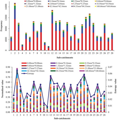
The FD of each sub-catchment was calculated based on the changes in the counting of boxes (Fig. 3). It should be noted that box-counting is a method of gathering data for analysing complex patterns by breaking a dataset, object, image, etc. into smaller and smaller pieces. The results showed that sub-catchment 8 obtained the highest FD (1.14). According to Fig. 1, its drainage network also had the highest number of branches and irregularities. In contrast, the drainage network of sub-catchment 4, with an FD of 0.89, had the fewest branches and irregularities.

Figure 3. An example of calculating the fractal dimension in sub-catchments

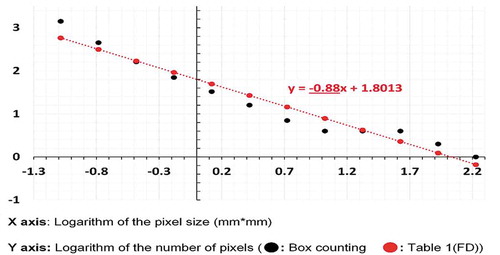
Table 4 shows that the correlation coefficient (R) between the FD of a drainage network and the box-counting estimate at all sub-catchments is higher than 61%, implying the accuracy of the FD at the river network. These findings are consistent with those of Zhang et al. (2015) and Malekinezhad et al. (2017), who also used the box-counting method. After obtaining the FD at each sub-catchment, the total area was divided into five classes based on HCA: very high (1.108–1.136), high (1.088–1.103), moderate (1.037–1.08), low (1.002–1.006), and very low (0.8875–0.9287) (Figs 4(a) and Figs 5(a)).

Table 4. Fractal dimension and its correlation coefficient (R) for the drainage network in sub-catchments

Sub-catchment no.	FD	R	Sub-catchment no.	FD	R
1	1.04	0.74	15	1.10	0.83
2	1.1	0.8	16	1.06	0.71
3	1.13	0.79	17	1.09	0.78
4	0.89	0.61	18	1.07	0.79
5	1.11	0.84	19	1.05	0.77
6	1.07	0.62	20	1.09	0.78
7	1.06	0.75	21	1.09	0.77
8	1.14	0.82	22	1.059	0.76
9	1.12	0.84	23	1.121	0.83
10	1.05	0.74	24	1.092	0.79
11	0.93	0.63	25	1.01	0.67
12	1.10	0.78	26	1.08	0.79
13	1.09	0.77	27	1.01	0.66
14	1.11	0.8	28	1.05	0.77

Figure 4. Mapping of sediment production hotspots using (a) FD, (b) EW, (c) SL, and (d) SC methods

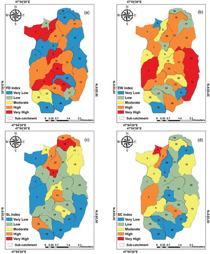
Figure 5. Clustering similar sub-catchments in terms of sediment production based on (a) FD, (b) EW, (c) SL, and (d) SC results

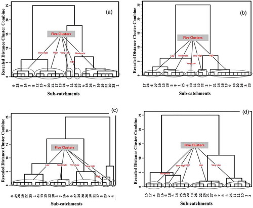
Sub-catchments 2 and 11 show the highest (0.06) and lowest (0.008) EW values, respectively. In other words, they are the sub-catchments with the most drainage network irregularities (or highest sediment yield) and the fewest drainage network irregularities (or the lowest sediment yield) (Fig. 6). Based on HCA, this section divided the total area into five classes with the following values: very high (0.056–0.065), high (0.039–0.049), moderate (0.026–0.034), low (0.02–0.02), and very low (0.008–0.016) (Figs 4(b) and Figs 5(b)).

Figure 6. Top: Schematic of a box-counting method to evaluate the presence of a drainage network at different sizes. Bottom: Normalized evaluation of the presence of a river network for a variety of sizes, and calculating their entropy

3.2 Analysis of SL and SC methods

After calculating the SL for the river network at all sub-catchments and generalizing it to all sub-catchment surfaces using the IDW method, the standard deviations of SL values at those sub-catchments were compared. The highest SD (3661.635) was observed in Sub-catchment 4. Sub-catchments 2 and 3 produced the lowest and highest SL values (0 and 35 116.25), respectively, among all sub-catchments (Fig. 7).

Figure 7. Top: SL and SC values in sub-catchments; bottom: standard deviation (SD) of SL and SC indices in sub-catchments

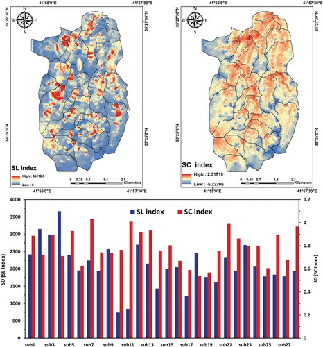
The SL internal interval variations of Sub-catchment 4 were used to prepare the classification table. The minimum SL, at Sub-catchment 2 (0), and the maximum SL, at Sub-catchment 3 (35 116.26), were used as boundary conditions in the SL classification table for all sub-catchments. After classifying the sub-catchments into five classes based on SL values, namely very low (0–3653.4), low (3653.4–6813.11), moderate (6813.11–10 071.55), high (10 071.55–14 514.89), and very high (14 514.89–35 116.257), a value ranging from 0.04 to 0.52 was assigned to each class at every sub-catchment using AHP (Table 2). Finally, these ranges were divided into five sediment yield groups, namely very low (3.75–4.40), low (4.53–4.9), moderate (5.03–5.22), high (5.72–6.59), and very high (7.77–7.77) (Figs 5(c) and Figs 6). Table A1 presents the SL-based clustering algorithm details.

Similar to the sub-catchment prioritization with the SC method, the internal values of the classification table were extracted from Sub-catchment 7; also, the highest and lowest values of this table were extracted from sub-catchments 27 and 28, respectively (Fig. 7). Afterwards, the sub-catchments were divided into five classes, namely very low (−5.23 to −1.84), low (−1.84 to −1.1), moderate (−1.1 to −0.35), high (−0.35 to 0.46), and very high (0.46 to 2.31), based on the SC values, which were assigned to a specific number using AHP. These numbers were clustered into very low (11.92–21.24), low (23.12–28.46), moderate (30.23–31.87), high (33.69–36.94), and very high (40.01–40.97) sediment yield susceptibility (Figs 4(d) and Figs 5(d)). Table A2 shows the specifications of the SC clustering algorithm. However, it is important to note that these results can vary at the hillslope scale, due to the connectivity processes and different land management or environmental conditions (soils, parent material, vegetation, etc.) (Bracken et al. 2015, Cossart et al. 2017, Rodrigo-Comino et al. 2018). This depends on the scale used.

3.3 Comparison and assessment of accuracy of irregular and regular methods

To compare and assess the accuracy of each sediment yield hotspot and set priority for layers prepared by the above methods, this study used the EPM model. To evaluate the results of the total sediment (Gs) obtained from the EPM model (Table 3), the volume of the check dams’ sediments (VS) in the sub-catchments (Fig. 1), which were collected from the database of the General Department of Natural Resources of Hamadan Province, was used. There is always a difference between observed and estimated sediment data (i.e. VS and Gs) in nature, which may be due to the deposition of sediments along the transfer way, or sediment trapping behind vegetation or in holes in the catchment (Imeson and Prinsen 2004, Najafi et al. 2020). Therefore, to determine the best-performed Gs and VS curve, different regression fitting procedures were applied. The results of a simple linear regression study showed high correlations were established, as in Equation (9)(9) $VS=0.227Gs-223$(9) .

In this regard, various statistical criteria, viz. coefficient of determination (R²), a significant p-value (P), root mean square error (RMSE), and coefficient of efficiency (CE), were then applied to evaluate the fitness (Sadeghi et al. 2012). The values obtained for R², P, CE, and RMSE using Equation (9)(9) $VS=0.227Gs-223$(9) were, respectively, 0.79, 0.02, 0.72, and 0.007. Therefore, the efficiency of the EPM model in the Ilanlu catchment has been confirmed, and it can be used to evaluate the EW, FD, SL, and SC methods.

(9) $VS=0.227Gs-223$(9)

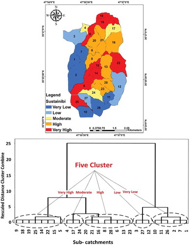
In the following, the EPM values for each sub-basin from the methods used were classified into five sediment production susceptibility levels, i.e. very high, high, moderate, low and very low, based on the HCA method (Fig. 8). Then, the output of the methods used was superimposed on the output of the EPM model. In the FD method, eight sub-catchments were found in common with the output of the EPM model. In the EW method, 10 sub-catchments were found in common with EPM (Table 5).

Table 5. The number of sub-catchments located in different sediment transportation zones

	Very high	High	Moderate	Low	Very low
EPM	5, 15, 14, 22, 25, 19, 9, 18	6, 8, 13, 16, 20, 21, 23, 28	24, 17, 4	12, 27, 3	26, 11, 10, 7, 2, 1
EW	2, 12, 22	3, 7, 9, 13, 14, 16, 18, 20, 21, 23, 26	1, 5, 8, 15, 25, 28	6, 17, 19, 24, 27	4, 10, 11
FD	3, 5, 8, 9, 14, 23	2, 12, 13, 15, 17, 20, 21, 24	25, 27	1, 6, 7, 10, 16, 18, 19, 22, 26, 28	4, 11
SL	4	2, 5, 23	3, 7, 9, 12, 16, 18	1, 8, 13, 15, 19, 21, 22, 24, 25, 28	6, 10, 11, 14, 17, 20, 26, 27
SC	6, 18	5, 14, 19, 20, 25	4, 15, 16, 17, 23	7, 8, 9, 13, 21, 22, 24, 27, 28	1, 2, 3, 10, 11, 12, 26

Figure 8. Top: Mapping of sediment production hotspots. Bottom: Clustering similar sub-catchments in terms of sediment production using the EPM model

These results show the good accuracy of the FD and EW methods in sediment yield priority. A major reason for the superiority of the EW method over the FD method could be the assessment changes in the presence of drainage networks in different box sizes. The regression method in FD is used to assess this dynamic. Since these changes have a log-log relationship, a slight change in linear regression slope causes a large uncertainty in the final sediment yield mapping. For the assessment of this behaviour using the EW method, the sum operator is used (Table 1). Therefore, this method is associated with lower uncertainty.

The results of the SL method showed that only sub-catchments 4 and 5 in classes of very high and high and sub-catchments 10 and 26 are common with the EPM model (Table 5). Our results indicate that the sub-catchments 4 and 5 and sub-catchments 10 and 26 have the maximum and minimum DH/DL (or slope degree) values, respectively. Although this method can demonstrate both stream power and sediment transportation, the inclination is the core factor in this regard (Table 1), as other authors have demonstrated in mountainous catchments (Nadal-Romero et al. 2014, Brandolini et al. 2016). SL is typically used in perturbation zones of active geodynamical settings. Therefore, in low-perturbation areas, the river network has a low SL, whereas the SL is higher in river networks located in areas with moderate and high subduction rates (El Hamdouni et al. 2008, Troiani et al. 2014, Gaidzik and Ramírez-Herrera 2017). In the SC index, Sub-catchment 5 is common with EPM model. This finding shows that this method achieved a 4% accuracy.

In the SC index, there are nine sub-catchments in common with EPM model (Table 5). There are two reasons why this method might have high accuracy. The first reason is the opposite of other methods, related to considering various parameters such as slope, roughness coefficient, upslope area and flow length. The second and more important reason is related to considering the linkage between upstream and downstream areas, which is called connectivity in hydrology studies, and which has not been considered with the other methods. Heckmann et al. (2015) recommended that in studies of flood, erosion, sediment yield and other hydrology studies, to produce high accuracy, it is necessary to consider connectivity indices. Recently, Rodrigo-Comino et al. (2020) demonstrated that this index could be even applied to smaller scales if in situ measurements are taken.

3.4 Challenges and other considerations

Overuse of natural resources can accelerate soil loss and leads to increased sediment load in streams which is reflected in problems within and beyond individual catchments (Li et al. 2020a, 2020b). Recognition of hotspot areas susceptible to sediment loss is, therefore, an essential element in designing effective and comprehensive strategies related to land management at the catchment scale, considering sediment yield and transport (Kiani-Harchegani and Sadeghi 2020, Najafi et al. 2020). Thus, identifying sedimentary hotspots in management concepts is especially important in developing countries, where high erosion and sediment delivery rates cause severe problems but there is a lack of information (Heckmann et al. 2018, Najafi et al. 2018).

Therefore, EW and FD (as irregular methods) and SL and SC (as regular ones) were evaluated as concepts in assessing the hydrological and erosional responses of watershed components having different natural and management characteristics. The results showed that they can be used as an effective screening tool for hydrological, erosional and sediment management. Such studies would meet the practical need for sediment management at different temporal and spatial scales. We consider that a greater understanding of the above methods and the interaction between soil erosion and sediment transport processes, as well as a better understanding of their spatiotemporal responses, would decrease uncertainties in interpreting sediment transport and sediment yield within catchments (Najafi et al. 2020).

4 Conclusion

This study used four common methods, namely EW and FD as irregular methods and SL and SC as regular methods, to prioritize sediment production hotspots in the study site. The soil erosion of each sub-catchment was measured using the aforementioned methods after dividing the case study area into 28 sub-catchments. The outputs were superimposed on the output results of the EPM model. The EW, followed by SC, FD, and SL, was most accurate in categorizing the sub-catchments from the viewpoint of susceptibility to sediment transportation and possible yield. These results support the superimposition method.

Although the results of the current study revealed the superiority of some methods over the others under investigation, each method has its pros and cons. Therefore, it is suggested to improve the performance of these methods or use a combination of them to help developing countries to foresee future and potential hazard risks. On the other hand, it is possible to apply these methods in other drainage networks that have a direct relationship between soil erosion and sediment production. This gives another relevant point to this research.

Disclosure statement

No potential conflict of interest was reported by the authors.

Appendix

Table A1. The SL-based clustering algorithm used in this study

Table A2. The clustering algorithm using the SC index

References

- Aga, A.O., Melesse, A.M., and Chane, B., 2020. An alternative empirical model to estimate watershed sediment yield based on hydrology and geomorphology of the Basin in data-scarce Rift Valley Lake Regions, Ethiopia. Geosciences, 10, 31. doi:https://doi.org/10.3390/geosciences10010031
- Al-Dulaimi, G.A. and Younes, M.K., 2017. Assessment of potable water quality in Baghdad City, Iraq. Air, Soil and Water Research, 10, 1178622117733441. doi:https://doi.org/10.1177/1178622117733441
- Alexakis, D.D., Hadjimitsis, D.G., and Agapiou, A., 2013. Integrated use of remote sensing, GIS and precipitation data for the assessment of soil erosion rate in the catchment area of “Yialias” in Cyprus. Atmospheric Research, 131, 108–124. doi:https://doi.org/10.1016/j.atmosres.2013.02.013
- Al-Wagdany, A., et al., 2020. Effect of the stream extraction threshold on the morphological characteristics of arid basins, fractal dimensions, and the hydrologic response. Journal of African Earth Sciences, 172, 103968. doi:https://doi.org/10.1016/j.jafrearsci.2020.103968
- Arabameri, A., Cerda, A., and Tiefenbacher, J.P., 2019. Spatial pattern analysis and prediction of gully erosion using novel hybrid model of entropy-weight of evidence. Water, 11 (6), 1129. doi:https://doi.org/10.3390/w11061129
- Ariza-Villaverde, A.B., Jiménez-Hornero, F.J., and Gutiérrez De Ravé, E., 2013. Multifractal analysis applied to the study of the accuracy of DEM-based stream derivation. Geomorphology, 197, 85–95. doi:https://doi.org/10.1016/j.geomorph.2013.04.040
- Bizzi, S. and Lerner, D.N., 2015. The use of stream power as an indicator of channel sensitivity to erosion and deposition processes. River Research and Applications, 31 (1), 16–27. doi:https://doi.org/10.1002/rra.2717
- Boltzmann, L. 1877. On the nature of gas molecules. The London, Edinburgh, and Dublin Philosophical Magazine and Journal of Science, 3(18), 320–320.
- Bracken, L.J., et al., 2015. Sediment connectivity: a framework for understanding sediment transfer at multiple scales. Earth Surface Processes and Landforms, 40 (2), 177–188. doi:https://doi.org/10.1002/esp.3635
- Brandolini, P., et al., 2016. Response of terraced slopes to a very intense rainfall event and relationships with land abandonment: a case study from Cinque Terre (italy). Land Degradation and Development, 29 (3), 630–642. doi:https://doi.org/10.1002/ldr.2672
- Burbank, D. and Anderson, R., 2001. Chapter 9. Deformation and geomorphology at intermediate time scales. In Tectonic geomorphology. Oxford: Blackwell Science, 175–199.
- Chen, L., et al., 2019. A fractal model of hydraulic conductivity for saturated frozen soil. Water, 11 (2), 369. doi:https://doi.org/10.3390/w11020369
- Cossart, É., Lissak, C., and Viel, V., 2017. Geomorphic analysis of catchments through connectivity framework: old wine in new bottle or efficient new paradigm? Géomorphologie : relief, processus. Environment, 23, 281–287.
- De Cola, L. and Lam, -N.S.-N., 2002. A fractal paradigm for geography. Fractals in Geography. New Jersey: PTR Prentice-Hall, Inc., 75–83.
- De Freitas Sampaio, L., Crestana, S. and Rodrigues, V. G. S. 2019. Study of gully erosion in South Minas Gerais (Brazil) using fractal and multifractal analysis. ed. IAEG/AEG Annual Meeting Proceedings, San Francisco, California, 2018—Volume 6, 217–222.
- Dou, W., et al., 2020. Pore structure, fractal characteristics and permeability prediction of tight sandstones: a case study from Yanchang formation, Ordos Basin, China. Marine and Petroleum Geology, 104737.
- Efthimiou, N. and Lykoudi, E., 2016. Soil erosion estimation using the EPM model. Bulletin of the Geological Society of Greece, 50 (1), 305–314. doi:https://doi.org/10.12681/bgsg.11731
- El Hamdouni, R., et al., 2008. Assessment of relative active tectonics, southwest border of the Sierra Nevada (southern Spain). Geomorphology, 96 (1–2), 150–173. doi:https://doi.org/10.1016/j.geomorph.2007.08.004
- Estrany, J., et al., 2019. Hydrogeomorphological analysis and modelling for a comprehensive understanding of flash-flood damaging processes: the 9th October 2018 event in North-eastern Mallorca. Natural Hazards and Earth System Sciences Discussion, 2019, 1–36.
- Fiorentino, M., Claps, P., and Singh, V.P., 1993. An entropy-based morphological analysis of river basin networks. Water Resources Research, 29 (4), 1215–1224. doi:https://doi.org/10.1029/92WR02332
- Gaidzik, K. and Ramírez-Herrera, M.T., 2017. Geomorphic indices and relative tectonic uplift in the Guerrero sector of the Mexican forearc. Geoscience Frontiers, 8 (4), 885–902. doi:https://doi.org/10.1016/j.gsf.2016.07.006
- García‐Ruiz, J.M., et al., 2017. Ongoing and emerging questions in water erosion studies. Land Degradation and Development, 28 (1), 5–21. doi:https://doi.org/10.1002/ldr.2641
- Hamza, V., Prasannakumar, V. and Pratheesh, P. 2019. Modelling and interpretation of channel profile anomalies through stream length gradient (SL) indexes and GIS: A case study from the Vamanapuram River, Kerala, India. Environmental Research, Engineering and Management, 75(2), 60–73.
- Hassan, M.K. and Kurths, J., 2002. Can randomness alone tune the fractal dimension? Physica A: Statistical Mechanics and Its Applications, 315 (1–2), 342–352. doi:https://doi.org/10.1016/S0378-4371(02)01242-6
- Heckmann, T., et al. 2015. Indices of hydrological and sediment connectivity-state of the art and way forward. Paper presented at the EGU General Assembly Conference Abstracts. Held 12–17 April, 2015 in Vienna, Austria. id.12793.
- Heckmann, T., et al., 2018. Indices of sediment connectivity: opportunities, challenges and limitations. Earth-Science Reviews, 187, 77–108.
- Hu, Q., et al., 2020. Machine learning and fractal theory models for landslide susceptibility mapping: case study from the Jinsha River Basin. Geomorphology, 351, 106975. doi:https://doi.org/10.1016/j.geomorph.2019.106975
- Ildoromi, A.R., et al., 2019. Application of multi-criteria decision making and GIS for check dam layout in the Ilanlu Basin, Northwest of Hamadan Province, Iran. Physics and Chemistry of the Earth, Parts A/B/C, 114, 102803. doi:https://doi.org/10.1016/j.pce.2019.10.002.
- Imeson, A.C. and Prinsen, H.A.M., 2004. Vegetation patterns as biological indicators for identifying runoff and sediment source and sink areas for semi-arid landscapes in Spain. Agriculture, Ecosystems & Environment, 104 (2), 333–342.
- Jaafari, A., et al., 2014. GIS-based frequency ratio and index of entropy models for landslide susceptibility assessment in the Caspian forest, northern Iran. International Journal of Environmental Science and Technology, 11 (4), 909–926. doi:https://doi.org/10.1007/s13762-013-0464-0
- Kalantari, Z., et al., 2019. Assessing flood probability for transportation infrastructure based on catchment characteristics, sediment connectivity and remotely sensed soil moisture. Science of Total Environment, 661, 393–406. doi:https://doi.org/10.1016/j.scitotenv.2019.01.009
- Keum, J., et al., 2017. Entropy applications to water monitoring network design: a review. Entropy, 19 (11), 613. doi:https://doi.org/10.3390/e19110613
- Kiani-Harchegani, M. and Sadeghi, S.H., 2020. Practicing land degradation neutrality (LDN) approach in the Shazand Watershed, Iran. Science of Total Environment, 698, 134319. doi:https://doi.org/10.1016/j.scitotenv.2019.134319
- Kiani-Harchegani, M., Sadeghi, S.H., and Asadi, H., 2018. Comparing grain size distribution of sediment and original soil under raindrop detachment and raindrop-induced and flow transport mechanism. Hydrological Sciences Journal, 28 (1), 312–323. doi:https://doi.org/10.1080/02626667.2017.1414218
- Kouli, M., Soupios, P., and Vallianatos, F., 2009. Soil erosion prediction using the Revised Universal Soil Loss Equation (RUSLE) in a GIS framework, Chania, Northwestern Crete, Greece. Environmental Geology, 57 (3), 483–497.
- Kusák, M. 2014. Methods of fractal geometry used in the study of complex geomorphic networds. AUC Geographica, 49(2), 99–110.
- Li, J., et al., 2019. Combining box counting-dimension with a fuzzy synthetic evaluation model based quantitative evaluation on soil and water rrosion of Lake Dianchi Basin, China. ed. IOP Conference Series: Materials Science and Engineering, 052063.
- Li, Y., et al., 2020a. Anthropogenic disturbances and precipitation affect Karst sediment discharge in the nandong underground river system in Yunnan, Southwest China. Sustainability, 12 (7), 3006. doi:https://doi.org/10.3390/su12073006
- Li, Y., et al., 2020b. Evaluation of soil erosion and sediment deposition rates by the 137Cs fingerprinting technique at different hillslope positions on a catchment. Environmental Monitoring and Assessment, 192 (11), 717. doi:https://doi.org/10.1007/s10661-020-08680-w
- Lin, G.-F. and Chen, L.-H., 2006. Identification of homogeneous regions for regional frequency analysis using the self-organizing map. Journal of Hydrology, 324, 1–9.
- Llena, M., et al., 2019. The effects of land use and topographic changes on sediment connectivity in mountain catchments. Science of Total Environment, 660, 899–912.
- López-Vicente, M., et al., 2013. Predicting runoff and sediment connectivity and soil erosion by water for different land use scenarios in the Spanish Pre-Pyrenees. Catena, 102, 62–73.
- López-Vicente, M., et al., 2015. Assessment of soil redistribution at catchment scale by coupling a soil erosion model and a sediment connectivity index (Central Spanish Pre-Pyrenees). Cuadernos de investigación geográfica/Geography Research Letters, 127–147.
- Mahoney, D.T., Fox, J.F., and Al Aamery, N., 2018. Watershed erosion modeling using the probability of sediment connectivity in a gently rolling system. Journal of Hydrology, 561, 862–883.
- Malekinezhad, H., et al., 2017. Flood hazard mapping using fractal dimension of drainage network in Hamadan City, Iran. Journal of Environmental Engineering and Science, 12 (4), 86–92.
- Mandelbrot, B., 1967. How long is the coast of Britain? Statistical self-similarity and fractional dimension. Science, 156 (3775), 636–638.
- Marçal, M., Brierley, G., and Lima, R., 2017. Using geomorphic understanding of catchment-scale process relationships to support the management of river futures: Macaé Basin, Brazil. Applied Geography, 84, 23–41.
- Martínez-Mena, M., Deeks, L., and Williams, A., 1999. An evaluation of a fragmentation fractal dimension technique to determine soil erodibility. Geoderma, 90 (1–2), 87–98.
- Moussi, A., et al., 2018. GIS-based analysis of the stream length-gradient index for evaluating effects of active tectonics: a case study of Enfidha (North-East of Tunisia). Arabian Journal of Geosciences, 11 (6), 123.
- Nadal-Romero, E., et al., 2014. Effects of slope angle and aspect on plant cover and species richness in a humid Mediterranean badland. Earth Surface Process of Landforms, 39, 1705–1716. doi:https://doi.org/10.1002/esp.3549
- Najafi, S., et al., 2020. Sediment connectivity concepts and approaches. Catena, 196, 104880.
- Najafi, S., Sadeghi, S.H.R., and Heckmann, T., 2018. Analyzing structural sediment connectivity pattern in a Taham watershed, Iran. Journal of Watershed Engineering and Management, 10 (2), 192.203. (In Persian). doi:https://doi.org/10.22092/IJWMSE.2018.116466
- Nasre, R., et al., 2013. Soil erosion mapping for land resources management in Karanji watershed of Yavatmal district, Maharashtra using remote sensing and GIS techniques. Indian Journal of Soil Conservation, 41 (3), 248–256.
- Noori, H., Siadatmousavi, S.M., and Mojaradi, B., 2016. Assessment of sediment yield using RS and GIS at two sub-basins of Dez Watershed, Iran. International Soil and Water Conservation Research, 4, 199–206.
- Nur, A.A., et al., 2016. Fractal characteristics of geomorphology units as Bouguer anomaly manifestations in Bumiayu. Central Java, Indonesia: IOP Publishing, 012019.
- Ouarda, T., et al., 2008. Intercomparison of regional flood frequency estimation methods at ungauged sites for a Mexican case study. Journal of Hydrology, 348 (1–2), 40–58.
- Piégay, H., et al., 2005. A review of techniques available for delimiting the erodible river corridor: a sustainable approach to managing bank erosion. River Research and Applications, 21 (7), 773–789.
- Poeppl, R.E., et al., 2019. Combining soil erosion modeling with connectivity analyses to assess lateral fine sediment input into agricultural streams. Water, 11 (9), 1793.
- Pournader, M., et al., 2018. Spatial prediction of soil erosion susceptibility: an evaluation of the maximum entropy model. Earth Science Informatics, 11 (3), 389–401.
- Prosser, I.P., et al., 2001. Corrigendum to: large-scale patterns of erosion and sediment transport in river networks, with examples from Australia. Marine & Freshwater Research, 52 (5), 817.
- Rodrigo-Comino, J., et al., 2020. Integrating in situ measurements of an index of connectivity to assess soil erosion processes in vineyards. Hydrological Science Journal. doi:https://doi.org/10.1080/02626667.2020.1711914
- Rodrigo-Comino, J., Keesstra, S.D., and Cerdà, A., 2018. Connectivity assessment in Mediterranean vineyards using improved stock unearthing method, LiDAR and soil erosion field surveys. Earth Surface Processes and Landforms, 43, 2193–2206. doi:https://doi.org/10.1002/esp.4385
- Sadeghi, S.H.R., Kiani-Harchegani, M., and Younesi, H.A., 2012. Suspended sediment concentration and particle size distribution, and their relationship with heavy metal content. Journal of Earth System Science, 121 (1), 63–71.
- Sandercock, P. and Hooke, J., 2011. Vegetation effects on sediment connectivity and processes in an ephemeral channel in SE Spain. Journal of Arid Environments, 75 (3), 239–254.
- Sepehri, M., et al. 2018. Suburban flood hazard mapping in Hamadan City, Iran. Proceedings of the Institution of Civil Engineers - Municipal Engineer, 1–25.
- Shannon, C., 1948. A mathematical theory of communication. The Bell System Technical Journal, 27 (3), 379–423.
- Sherriff, S. C., et al. 2019. Influence of land management on soil erosion, connectivity, and sediment delivery in agricultural catchments: Closing the sediment budget. Land Degradation & Development.
- Shit, P.K., Nandi, A.S., and Bhunia, G.S., 2015. Soil erosion risk mapping using RUSLE model on jhargram sub-division at West Bengal in India. Modeling Earth Systems and Environment, 1 (3), 28.
- Snelder, T.H. and Biggs, B.J., 2002. Multiscale river environment classification for water resources management 1. JAWRA Journal of the American Water Resources Association, 38 (5), 1225–1239.
- Snow, R.S., 1989. Fractal sinuosity of stream channels. Pure and Applied Geophysics, 131 (1–2), 99–109.
- Sougnez, N., Van Wesemael, B., and Vanacker, V., 2011. Low erosion rates measured for steep, sparsely vegetated catchments in southeast Spain. Catena, 84, 1–11.
- Stosic, T., Stosic, B., and Singh, V.P., 2017. Optimizing streamflow monitoring networks using joint permutation entropy. Journal of Hydrology, 552, 306–312.
- Su, H.T. and You, G.J.Y., 2014. Developing an entropy-based model of spatial information estimation and its application in the design of precipitation gauge networks. Journal of Hydrology, 519, 3316–3327.
- Troiani, F., et al., 2014. Spatial analysis of stream length-gradient (SL) index for detecting hillslope processes: a case of the Gállego River headwaters (Central Pyrenees, Spain). Geomorphology, 214, 183–197.
- Troiani, F., et al., 2017. Stream Length-gradient Hotspot and Cluster Analysis (SL-HCA) to fine-tune the detection and interpretation of knickzones on longitudinal profiles. Catena, 156, 30–41.
- Troiani, F. and Della Seta, M., 2008. The use of the stream length–gradient index in morphotectonic analysis of small catchments: a case study from Central Italy. Geomorphology, 102, 159–168.
- Turnbull, L. and Wainwright, J., 2019. From structure to function: understanding shrub encroachment in drylands using hydrological and sediment connectivity. Ecological Indicators, 98, 608–618.
- Xu, Y., et al. 2014. Fractal model for surface erosion of cohesive sediments. Fractals, 22(3), 1440006.
- Yang, S.-Y., et al., 2019. Characterization of landslide distribution and sediment yield in the TsengWen River Watershed, Taiwan. Catena, 174, 184–198.
- Yao, J.-B., et al., 2020. Drought analysis based on the information diffusion and fractal technology, a case study of winter wheat in China. Applied Engineering in Agriculture. doi:https://doi.org/10.13031/aea.13829.
- Yegemova, S., et al., 2018. Identifying the key information and land management plans for water conservation under dry weather conditions in the border areas of the Syr Darya River in Kazakhstan. Water, 10, 1754. doi:https://doi.org/10.3390/w10121754
- Zhang, K., et al., 2020. Comparison of fractal models using NMR and CT analysis in low permeability sandstones. Marine and Petroleum Geology, 112, 104069.
- Zhang, S., et al., 2017. The influence of changes in land use and landscape patterns on soil erosion in a watershed. Science of Total Environment, 574, 34–45.
- Zhang, S., Guo, Y., and Wang, Z., 2015. Correlation between flood frequency and geomorphologic irregularity of rivers network–a case study of Hangzhou China. Journal of Hydrology, 527, 113–118.
- Zhou, T., et al., 2020. Fractal analysis of power grid faults and cross correlation for the faults and meteorological factors. IEEE Access, 8, 79935–79946.