Water stress & water salience: implications for water supply planning

ABSTRACT

Water stress prompts a durable reduction in water demand under some circumstances. This demand reduction has the potential to alter the benefits and costs of demand- and supply-side alternatives in water supply planning. This paper takes a socio-hydrological approach to assess the implications of this feedback, in the context of Las Vegas, Nevada. This application demonstrates feasibility first by developing and testing a novel model of water salience as a function of proximity to water supply thresholds, and then linking modules to account for feedback between subsystems. Lastly, by comparing this model to a water use scenario model to assess system performance under a range of future conditions and potential responses, this work illustrates the trade-offs between scenarios and the socio-hydrological approach. This model, while specific to Las Vegas, demonstrates a prototypical modeling framework capable of examining water supply–demand interactions by incorporating water stress-driven conservation.

KEYWORDS:

• water supply
• demand management
• systems analysis
• socio-hydrology
• planning

Editor S. Archfield; Associate editor G. di Baldassare

1 Introduction

At the height of the Millennium Drought, the state of Victoria, Australia, entered into a 30-year contract with the Victorian Desalination Plant (State Government of Victoria 2015). The plant, which can meet one third of the city’s annual demand, was constructed at a capital cost of AUD 3.5 billion in 2012 and immediately put into standby mode as the drought had abated and demand had dropped. While there is value in redundancy, this expensive stranded asset raises questions about the methods that led to a large plant over modular and staged construction or lower cost–demand management (Turner et al. 2016).

In water supply planning, there is growing awareness that the hydro-climatic system is dynamic and changing (Milly et al. 2008, Vogel et al. 2011), and that water managers are not well served by a single water use projection. However, despite methodological advances exploring a broader range of climatic and demand scenarios (Lempert and Groves 2010, Brown et al. 2012), planning methods do not account for the adaptability and feedback inherent in water management (de Neufville and Scholtes 2011). At the urban scale, demand management is an important component of this adaptability.

Dynamic socio-hydrologic modeling has been proposed to address this challenge and is an important complement to existing modeling practices (Sivapalan et al. 2012, Montanari et al. 2013, Thompson et al. 2013). While scenarios can also be used to explore water use changes with less modeling effort, there are distinct advantages to building demand dynamics, including both their biophysical and institutional drivers, into a systems model. Explicitly modeling the dynamics of both institutional and biophysical systems enables exploration of the impact of path dependencies not easily identifiable in a typical scenario-generation process. The Las Vegas, Nevada, metropolitan area water system is used as a test case to assess this exploration.

Previous work has shed light on the drivers of water use change (Mayer et al. 2004, Wentz and Gober 2007, Schleich and Hillenbrand 2009, Coomes et al. 2010, Russell and Fielding 2010, Mini et al. 2015, Hester and Larson 2016, Brelsford and Abbott 2017). Specifically, several researchers have observed that under some circumstances, water users respond to water stress with demand reduction and that a portion of that demand reduction is durable (Gonzales and Ajami 2017, Quesnel and Ajami 2017, Di Baldassarre et al. 2018, Garcia and Islam 2018). Garcia and Islam (2018) document the development and testing of a per capita water use model for the Las Vegas Valley Water District (LVVWD) that captures this phenomenon. However, the implications of this phenomenon for water supply planning have not yet been assessed. To apply this type of model in practice requires developing a modeling framework that accounts for feedback between subsystems and reconciles issues of scale mismatch across subsystems (e.g. supply management vs. demand management), and requires developing modules of additional subsystems.

The objective of this paper is to build a full water supply systems model for LVVWD to assess the benefits and limitations of this sociohydrological approach, that captures demand response to water stress in a planning context. There is an additional model development and computational workload associated with this approach. Additionally, the broader model scope increases the challenges of addressing equifinality and maintaining parsimony (Hawkins 2004, Kumar 2011). These tradeoffs are merited if the analysis results in insights not found using water use scenarios.

This paper is organized as follows. In the next section we present the case of Las Vegas water management, describing both supply- and demand-side features. The following section documents the methodology applied to build and assess the model and to develop the scenarios and response alternatives. Then, we present the results of both model development and system performance under four scenarios, with and without supply- and demand-side responses using both the exogenous and endogenous water use modeling approaches. Finally, we discuss the model comparison including strengths, limitations, policy implications and next steps.

2 Case description

The Las Vegas metropolitan area is in the Mojave Desert in Southern Nevada. The LVVWD, a public water utility, serves the city of Las Vegas and the unincorporated areas of Clark County, Nevada (Fig. 1(a)). The LVVWD is just one entity in a multi-level network of water management. Water management in the Las Vegas metropolitan area is led by the Southern Nevada Water Authority (SNWA). The SNWA is a cooperative agency that coordinates water supply, conservation efforts and infrastructure development for the Las Vegas metropolitan area. Las Vegas is one of many areas dependent on the Colorado River, and allocation agreements span the seven basin states and Mexico. Since 1995, the SNWA, as Nevada’s largest user of Colorado River water, has been the negotiating party acting on behalf of the state (Ott Verburg 2010). Since the formation of the SNWA, member utilities (Fig. 1(b)) have coordinated their water deliveries and conservation policies (Mulroy 2008).

Figure 1. (a) Case location; (b) organizational hierarchy (SNWA = Southern Nevada Water Authority; LVVWD = Las Vegas Valley Water District); and (c) Lake Mead operational rule diagram

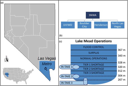
The Las Vegas water system consists of the portfolio of water supply managed by the SNWA, the demands served by the member utilities (Fig. 2(a)), and the storage, conveyance and treatment infrastructure. The primary source of water is Lake Mead, which accounts for 90% of supply; the remaining 10% is supplied by local groundwater (Fig. 2(c); SNWA 2009). By law, supply from the Colorado River is based on the Lake Mead water elevation, which changes due to stochastic inflows and upstream withdrawals (Fig. 2(b)). The SNWA extracts water from Lake Mead through three intake structures (Fig. 1(c)).

Figure 2. Case data: (a) monthly per capita water use in the LVVWD services area; (b) monthly Lake Mead water levels; (c) annual LVVWD cumulative banked groundwater volume (excluding AZ bank); (d) monthly percentage of media articles in the Las Vegas Review Journal on water issues

The drought in the early 2000s threatened the first intake structure. In 2005, construction began on a third and lower intake structure which was completed in 2015 (SNWA 2015). The SNWA can extract additional water beyond their consumptive water rights based on return flow credits. Return flow credits are created by discharging treated wastewater back into Lake Mead. Primary demands are generated by residents, the tourist industry and outdoor recreation (Dawadi and Ahmad 2013). Data on all variables was available for the full study period beginning in 1991 and ending in 2012 (Fig. 2). Further information on data types and sources is provided in Table 1.

Table 1. Data sources and characteristics

Variable	Frequency	Source	Units
Total Water Usage	Monthly	Las Vegas Valley Water District	Million Gallons
Surface Water Withdrawals	Monthly	US Bureau of Reclamation	Acre-Feet
Groundwater Pumping	Monthly	Nevada Division of Water Resources	Million Gallons
Banked Groundwater	Annual	Nevada Division of Water Resources, Southern Nevada Water Authority, Arizona Water Banking Authority	Million Gallons
Lake Powell Elevation	Monthly	US Bureau of Reclamation	Feet
Lake Mead Elevation	Monthly	US Bureau of Reclamation	Feet
Evaporation Loss from Lake Powell	Monthly	US Bureau of Reclamation	Feet
Evaporation Loss from Lake Mead	Monthly	US Bureau of Reclamation	Feet
LVVWD Population	Annual	Clark County	Persons
Tiered Water Rates	Monthly	Las Vegas Valley Water District	$/3790 L
Media Coverage	Monthly	Las Vegas Review-Journal	Normalized % of articles on water
Mean Temperature	Monthly	National Oceanic and Atmospheric Administration	°C

3 Methodology

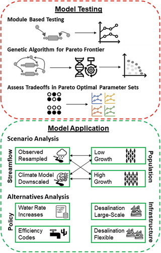
The methodology, summarized in Fig. 3, consists of three phases: model development, model testing and model application.

Figure 3. Project methodology

3.1 Model development

This analysis seeks to determine the benefits and limitations of including water use as an endogenous variable. As such, it is critical to include interactions between supply-side and demand-side management. Demand management is the responsibility of municipalities and utilities; the LVVWD is the largest of the Las Vegas metropolitan area water utilities. Therefore, the water use module is set up to incorporate the management options and behavior of the LVVWD. The SNWA and not the LVVWD, however, is primarily responsible for water supply management. The SNWA constructs and maintains water intake and conveyance infrastructure, conducts long-range planning and participates in negotiations with other Colorado River water users. Therefore, the supply module includes the surface and groundwater supply managed by the SNWA and the operational rules constraining SNWA actions.

Finally, streamflow into Lake Mead is influenced by land cover characteristics throughout the basin as well as upstream water usage. As the watershed is much larger than the Las Vegas metropolitan area, watershed properties are exogenous from decisions made at the city scale. Upstream and downstream water usage are also considered exogenous. Regional economic and demographic conditions influence water usage throughout the basin; therefore, upstream usage scenarios are coordinated with population growth scenarios in the Las Vegas metropolitan area.

The mismatch in the scale at which responsibility is vested for supply and demand management is addressed with a multi-level model structure. At the highest level, available surface water is computed at an annual time step by routing exogenous streamflow through a simplified reservoir system. Available groundwater is also computed annually based on groundwater rights and banked water. Water usage is computed monthly based on the LVVWD context (rates, codes, etc.). The LVVWD is used in place of the SNWA for water use computations because the important water management variables, such as water rates, are not constant throughout the SNWA service area. The water use is then scaled up to the total SNWA service area water use based on historical water use.

The implicit assumption in this approach is that both population growth and conservation policy implementation occur evenly across municipalities within the SNWA service area. This assumption is reasonable because conservation policies are coordinated between the SNWA member agencies (SNWA 1999). The plausibility of the population assumption depends on where future growth is concentrated in Clark County. If growth is proportionally split between the LVVWD service area (the City of Las Vegas and unincorporated suburban areas) and other municipalities (Henderson, North Las Vegas, etc.), this is a reasonable assumption. The impact of growth patterns on long-term water supply reliability can be explored by varying the percentage of SNWA used by the LVVWD with time. This is an important area of future work but is beyond the scope of the current analysis.

For comparison, two versions of the water supply system model are developed. The first version, termed the exogenous model, uses water consumption scenarios. The second version, termed the endogenous model, computes water consumption as an endogenous variable.

3.1.1 Reservoir operations

While there are many reservoirs along the Colorado River, the operation of two, Lake Mead and Lake Powell, is incorporated in this model as they are the largest reservoirs on the Colorado River. Lake Mead storage and operations are modeled because SNWA withdraws water directly from the reservoir. Lake Powell is modeled because the downscaled general circulation model (GCM)-projected streamflow generated by the Variable Infiltration Capacity (VIC) model is the equivalent of natural streamflow, and storage and operations are not taken into account (USBR 2012a). Therefore, Powell is included in the model to account for flow regulation upstream of Lake Mead.

Annual reservoir operations are modeled in accordance with the Criteria for Coordinated Long-Range Operation of Colorado River Reservoirs (US Bureau of Reclamation 1970), the Colorado River Interim Surplus Guidelines (Department of the Interior 2001), and the Colorado River Interim Guidelines for Lower Basin Shortages and the Coordinated Operations of Lake Powell and Lake Mead (Department of the Interior 2007). Monthly discharge from Lake Powell is computed based on the determined annual discharge and the average percentage of the annual volume discharged each month based on historical data (US Bureau of Reclamation 2016). Monthly withdrawal from Lake Mead is divided into two parts: lower basin usage and SNWA withdrawal. Lower basin usage is incorporated as an exogenous variable. SNWA withdrawal is determined by the quantity of water demanded, the maximum allowable usage based on reservoir level, and groundwater supply.

3.1.2 Groundwater operations

There are two main components to the groundwater module: groundwater rights and banked groundwater. The LVVWD holds 40,629 acre-feet in annual groundwater rights, and the City of North Las Vegas holds an additional 6201 acre-feet (SNWA 2015). These groundwater rights are pooled, as all SNWA member agencies collectively manage both surface and groundwater supply (SNWA 1995). A simple decision rule is used to simulate conjunctive management of surface and groundwater supply. Surface water is used first, and then if unmet demand remains, groundwater is used. While simplistic, this rule is consistent with the SNWA aim to maximize use of the Colorado River allocation (SNWA 2009).

The SNWA has access to three groundwater banks: the Arizona Water Bank, the California Water Bank and the Southern Nevada Water Bank. The Southern Nevada Water Bank has been operational since 1987, the Arizona Bank since 2004 and the California Bank since 2004 (SNWA 2009). Both excess surface water and unused groundwater rights can be banked. Banked groundwater can be accessed in any month and is used only if available surface water and groundwater rights are insufficient to meet demand. Based on the banking agreements, the SNWA can withdraw up to 30,000 acre-feet per year from the California Bank and up to 40,000 acre-feet per year from the Arizona Bank (SNWA 2009). For model calibration, water banked in Arizona is excluded as it was purchased, not generated from existing water resources. The SNWA projects a maximum recovery rate of 20,000 acre-feet per year from Southern Nevada Water Bank (SNWA 2015). Note that extractions from the Arizona and California Banks must be wheeled through Lake Mead.

3.1.3 Water use

The quantity of water demanded by the LVVWD service area each month is determined based on water rates, population growth coupled with code changes, and response to water stress. Both per capita water usage and total LVVWD water usage are computed. The water usage module, including testing and calibration, is discussed in depth in Garcia and Islam (2018). As described above, SNWA water usage is calculated from LVVWD usage using a factor based on historical water use data.

3.1.4 Water supply salience

Passing and implementing demand management policies, or other types of rule changes, require information about the state of the system as well as the alignment of attention and resources. Rule changes have both advocates and opponents, and successful passage and implementation have financial and political costs. Information about the system must therefore be salient as well as available to overcome these hurdles (Garcia et al. 2020). Salience describes the observation that disproportionate weight in decision-making is given to the part of the decision-making environment where attention is directed (Kahneman and Tversky 1979). Environmental events, including water stress, can increase the salience of environmental issues and, as a result, shift policymakers’ and consumers’ cost–benefit calculation (Bordalo et al. 2012, Dessaint and Matray 2015, Hand et al. 2015). Water salience may be an important motivator of per capita water usage change (Quesnel and Ajami 2017, Garcia and Islam 2018). For hypothesis testing and learning, data on the frequency of newspaper coverage of water supply issues can be used as a proxy for water salience (Treuer et al. 2017, Wei et al. 2017). However, to be able to incorporate conservation driven by spikes in water salience into future projections, a model of water salience is needed.

A water salience equation was developed by Garcia et al. (2016). There are three key components to this equation. First, there is the set of variables that drive increases in salience. Here, the ratio of the shortage volume to the total demand volume squared is used as it is proportional to shortage cost (Draper and Lund 2004). Second, under high levels of salience, only a significant event will substantially increase salience. The first term is multiplied by one minus the current salience to account for this asymptotic effect. Third, salience decays over time as event awareness declines (Di Baldassarre et al. 2013). A more detailed discussion can be found in Garcia et al. (2020).

(1) $\frac{d{M}_t}{dt}={\left(\frac{S_t}{D_t{P}_t}\right)}^2\frac{\left(1-M_t\right)}{\mathrm{\Delta }t}-{\mu }_s{M}_t$(1)

where S is shortage volume (L³/T), D is per capita usage (L³/T/person), P is population (person), Δt is the time step (T), M is salience (unitless) and μ_s is the salience decay rate (1/T).

While the shortage-based equation is theoretically reasonable, no shortages occurred in the Las Vegas area during the study period. This confirms previous studies that show that the water management field is risk averse and acts preemptively to avoid adverse outcomes (Farrelly and Brown 2011). Therefore, while a shortage event would likely increase salience significantly, the occurrence of shortages is rare in the urban developed context, so alternatives must be considered.

In the case of Las Vegas, decision makers and stakeholders have utilized information on reservoir levels, total supply and water usage in decision-making (SNWA 2005, 2014a). For example, in an advisory committee meeting, managers discussed with stakeholders how reservoir levels impact the amount of water the SNWA can legally use (SNWA 2014b). Further, a review of the media coding and coverage data (Fig. 2(b)) shows that peaks in salience occur during periods when drought conditions worsened, and topics covered – such as Lake Mead declines, drought and alternative water sources – reflect this (coded following the method described by Treuer et al. 2017).

From the case background and preliminary data analysis, two alternative salience equations are developed. First, salience changes are hypothesized to be driven by the approach to water supply thresholds. Second, salience changes are hypothesized to be driven by the magnitude of water supply declines. Equations developed for both hypotheses retain the asymptotic and decay rate features of the original shortage-based salience equation.

Thresholds are key features of the surface water supply for Las Vegas, as reservoir level-based allocation changes are codified (Department of the Interior 2001, 2007, US Bureau of Reclamation 2018) and the intake structures used to withdraw water from Lake Mead can only function at certain reservoir levels. The threshold is computed based on the distance between current reservoir levels and the nearest threshold triggering reduced withdrawals, normalized by the total distance between thresholds. The distance from a reservoir operations threshold will only influence the salience of water issues if it is sufficiently close to that threshold. Therefore, a baseline is subtracted from the initial normalized threshold distance:

(2) $\frac{d{M}_t}{dt}=T_t\frac{\left(1-M_t\right)}{\mathrm{\Delta }t}-{\mu }_s{M}_t$(2)

(3) $T_t=1-\frac{E_t-thres{h}_b}{thres{h}_a-thres{h}_b}$(3)

(4) $T_t=max\left(b,T_t\right)-b$(4)

where T is the threshold factor (unitless), E is the reservoir elevation (L), thresh_b is the nearest reservoir elevation below the current level that triggers a change in allocation (L), thresh_a is the nearest reservoir elevation above the current level that triggers a change in allocation (L), and b is the baseline normalized distance from a reservoir threshold (unitless). The decay rate, μ, and the baseline, b, are calibrated parameters.

Significant shifts in water supply garner public attention. For example, in Miami, Florida, newspaper coverage of water issues spiked when a change in groundwater rights and drought co-occurred (Treuer et al. 2017). However, this response is only anticipated when there is a decrease in supply. The relative, not absolute, magnitude of a supply change is hypothesized to be important, so the ratio between supply change and total water usage is employed:

(5) $\frac{d{M}_t}{dt}=\left(\frac{\mathrm{\Delta }{W}_t}{D_t{P}_t}\right)\frac{\left(1-M_t\right)}{\mathrm{\Delta }t}-{\mu }_s{M}_t$(5)

where ΔW is the year-to-year decrease in supply (L³/T); if there is no decrease this variable is set to zero.

3.2 Model testing

Model testing and parameter estimation are challenging in integrated system models, such as socio-hydrological models, due to the many coupled processes involved (Brun et al. 2001, Sivapalan and Blöschl 2015). One way of addressing this challenge is to dissemble the model into subcomponents for testing and improvement (Beck, 1999, Sivapalan and Blöschl 2015). As described above, the Las Vegas water supply systems model is composed of a series of modules (groundwater banking, water use, etc.). Where alternate versions of the modules are considered, the following statistical metrics are computed for comparison: root mean square error (RMSE), percent bias and relative Nash-Sutcliffe efficiency (rNSE) (Moriasi et al. 2015). Consistent with Garcia and Islam (2018), an alternate-year calibration method is used to address the challenge of selecting calibration and validation periods when there are fundamental differences between portions of the study period.

Once the component models are assessed, the full model is assembled and calibrated. The non-dominated sorting genetic algorithm (NSGA), as implemented in the Multiple Criteria Optimization Algorithms and Related Functions R package (Mersmann et al. 2020), is used to explore the parameter space. Minimizing the RMSE metric, applied to each of the modules, is the optimization target. There are five calibrated parameters in the integrated model: α (water use response parameter), rF (percentage of wastewater recovered as return flow), μ (salience decay rate), b (salience threshold) and σ (salience scaling factor). All other parameters in the model were specified directly from the data. Lower and upper bounds of each parameter (Table 2) were set based on module-by-module parameter estimation, and physical constraints (i.e. no more than 100% of wastewater can be recovered).

Table 2. Parameter ranges and optimal values

	α	rF	u	b	σ
Lower bound	0.010	1.500	0.010	0.050	0.001
Upper bound	1.000	2.000	0.950	0.950	1.000
Optimal	0.058	1.855	0.756	0.647	0.460

Performance of the model is assessed by testing the fit of monthly per capita water usage, monthly Lake Mead elevation, monthly water salience and annual banked groundwater (no monthly data was available), against the historical data using the RMSE metric. The performance of multi-objective optimization algorithms varies across multiple dimensions including accuracy and diversity. Mostafaie et al. (2018) evaluated the performance of four evolutionary algorithms in the context of hydrological modeling and found no algorithm performed best on all measures. However, the non-dominated sorting genetic algorithm (NSGA-II) performed best on diversity and was therefore selected for this study. Additionally, NSGA-II has been applied successfully to hydrological modeling and water systems analysis (e.g. Dumedah et al. 2010, Kasprzyk et al. 2013, Zhang et al. 2017, Peng et al. 2018).

Based on guidance from Siriwardene and Perera (2006), the NSGA-II is run with a population size of 100 for 50 generations using the MCO R package (Mersmann et al. 2014). The resulting pareto optimal population is narrowed by normalizing the RMSE values for all four variables and screening out parameter sets with values above −1 of normalized RMSE for any variable. In effect, this focuses the manual search on parameter sets that have relatively high (though likely not the highest) performance for each parameter. After screening, the remaining parameter sets were explored, through a review of plots and a suite of statistical metrics (RMSE, percent bias, relative NSE and correlation coefficients).

3.3 Model application

After testing and revision, the model is used to evaluate performance under plausible future conditions, first under the assumption of no policy response and then with a series of possible responses. The scenario period extends from 2015 to 2060. The supply and demand scenarios used were developed by the US Bureau of Reclamation (USBR) as part of a study on the future of the Colorado River Basin. Two types of streamflow scenarios are applied here: observed resampled and downscaled climate model projections. The downscaled streamflow was previously derived from low (B1), medium (A1B) and high (A2) emission scenarios (USBR 2012b). The three emission scenarios were run in 16 GCMs, each with multiple initial conditions, resulting in a total of 112 projections; bias correction and spatial downscaling were applied before running the VIC hydrological model to generate streamflow scenarios (Christensen and Lettenmaier 2007, USBR 2012c). The GCMs and emission scenarios selected have been vetted by the USBR for use in regional streamflow studies and are all considered equally likely.

A streamflow regime is characterized by its mean, variability and trends. As the streamflow realizations can vary significantly within a streamflow regime, an ensemble of realizations was used to test the system performance for each streamflow regime. The ensemble of streamflow traces for observed streamflow was developed using the indexed sequential method, a simple bootstrapping method, to sample 45-year subsets of streamflow. This method is based on the assumption that the time series “wraps around” at the end (USBR 2012a). The subset is sampled randomly by selecting the starting point using the Monte Carlo technique, with each starting point being equally likely. As the downscaled GCM-projected streamflow sequences are progressive, the projections must be applied according to their associated dates, and the indexed sequential method is inappropriate. Therefore, sequences are selected using the Monte Carlo technique. Figure 2(a) shows the LOESS (LOcally WEighted Scatter-plot Smoother) and standard error of the sampled streamflow sequences.

The USBR developed four scenarios of population growth and water use in the basin: current projected, slow growth, rapid growth and enhanced environment (USBR 2012b). In this analysis we use two water usage scenarios, slow growth and rapid growth, representing lower and upper bounds. The water use was projected separately for each state in the basin, but in this work it was aggregated to the level of the upper and lower basin, with the exception of the Las Vegas metro area which was projected separately but assumed to follow the same trend as the state of Nevada as a whole. From the USBR growth scenarios, we employ the water use for the rest of the basin and the population growth for the Las Vegas Metro area. For the exogenous model, we pair the USBR population project with a per capita water use projection from the SNWA (SNWA 2015). Combining the streamflow and population scenarios results in four unique scenarios, with many possible streamflow sequences within these scenarios (Figure 4).

Figure 4. Streamflow and population scenarios: (a) LOESS and standard error of sampled streamflow generated from downscale GCM projections and resampled observed streamflow using the index sequential method; (b) high and growth population scenarios

While physically water constrained, Las Vegas has both supply- and demand-side options to decrease water stress and increase reliability. One supply-side option discussed by local stakeholders is the construction of a desalination plant in California or Mexico. Financing a desalination plant in either California or Mexico in exchange for a greater share of Colorado River water is feasible but still leaves Las Vegas vulnerable to shortages given the structure of both legal agreements and existing infrastructure (Mulroy 2008). The desalination policy assumes the construction of a plant with a capacity of 18 million gallons per year, resulting in an addition 18 million gallons per year of Colorado River water for Las Vegas.

To assess the impact of alternative decision rules, two desalination alternatives are considered. The first is to build the entire plant capacity when the demand-to-supply ratio first rises above 0.9. The second is to build one third of the ultimate capacity when the water stress metric (demand divided by supply) first rises above 0.9, and to add the rest of the capacity in two phases if and when the water stress metric again exceeds 0.9. As stated above, there is a delay between the decision to pursue desalination and project completion. Under typical circumstances a desalination plant would take several years to design, permit and build. Based on projects such as the Carlsbad Desalination Plant in San Diego, California, this time is optimistically estimated to be 10 years. Therefore, this analysis assumes a 10-year delay between decision and implementation for the first phase; subsequent phases are assumed to come online after only 3 years, based on the premise that permitting for the ultimate capacity will be completed in the first phase. This analysis focuses on the timing of desalination, the type of conservation policy and the ability to address Las Vegas’ long-term water concerns.

On the demand side, some conservation gains have been realized but room for improvement remains (Cooley et al. 2007), and this strategy can be implemented in the short to medium term, although the time to take effect varies. Fast conservation measures such as price increases can impact water use within a few months. Slow conservation measures such as changes to building and landscaping codes can be implemented quickly but take effect incrementally as properties are rebuilt or the city expands.

Water usage decreases as water rates rise in proportion to the local elasticity of demand. In practice, water rates are increased both to control demands when the utility is water stressed and to cover costs as expenses rise. A decision rule is used to simulate the management response to changes in water stress; for the current application financially motived rate changes are ignored. The effective marginal water rate is increased by 10% if water stress exceeds 0.9; the rate is decreased by 10% if the water stress falls below 0.5. Note that this assumes no change to the tiered structure of water rates. It is politically difficult to raise water rates, as the SNWA and LVVWD demonstrated in 2012 (SNWA 2013). The political challenges of rate increases are not dealt with in depth here, but frequency of rate changes is limited to once per year to avoid simulating unrealistic management patterns.

Water codes, including building and landscape codes, set the required efficiency of new construction. Building codes specify efficiency requirements for fixtures such as showers and toilets, while landscape codes specify allowable turf area, irrigation technology and climate-appropriate plantings. Code changes are implemented in the model as planned alternatives, not as decision rules, as they typically respond to long-term trends, not short-term indicators. Two code-tightening alternatives are considered: moderate and aggressive. For the moderate alternative, in 2020 there is a 6.3% increase in code efficiency (equivalent to a 10 gpcpd decrease in newly constructed homes) and in 2030 there is a further 10% efficiency increase. Under the aggressive alternative, in 2020 there is a 9.4% increase in code efficiency (equivalent to a 15 gpcpd decrease in newly constructed homes) and in 2030 a further 13.8% efficiency increase.

The system performance is evaluated under the business as usual (BAU) case and the detailed responses using two metrics: water supply stress index (WaSSI) and reliability. WaSSI is the ratio of the quantity of water demanded to the available water supply in a single time step. Following the method described by Treuer et al. (2017), the available supply considers all water sources (i.e. stored water, groundwater) constrained by the applicable rules, regulations and infrastructure capacities. Reliability is defined as the percentage of time steps in which WaSSI is below 0.9 (i.e. when the system has a buffer of less than 10% between supply and demand).

4 Results

The following section presents results of model testing and application to assess the impacts of streamflow and demographic scenarios and potential responses.

4.1 Model testing

4.1.1 Module testing and parameter estimation

The water salience functions are tested against observed water salience as measured by the normalized percentage of articles on the topic of water supply in the Las Vegas Review Journal. The threshold salience function captures the timing and magnitude of the largest salience increases during the study period (Fig. 5(a)). The supply change salience function matches the timing but overestimates the magnitude of the smaller salience increase (Fig. 5(b)). The two functions differ little in RMSE, and both show significant variation in percent bias between calibration and validation periods (Table 3). However, the threshold function has significantly higher correlation. A discussion of water use module testing and calibration can be found in Garcia and Islam (2018). Reservoir and groundwater operation modules were also tested individually, and their performance is summarized in the Supplemental material.

Table 3. Salience function performance statistics

Calibration statistics
Salience Equation	RMSE	% Bias	Corr.
f(Threshold distance)	0.002	57.5	0.812
f(Water supply volume change)	0.003	9.7	0.234
Validation statistics
Salience Equation	RMSE	% Bias	Corr.
f(Threshold distance)	0.002	17.0	0.809
f(Water supply volume change)	0.002	−67.6	0.400

Figure 5. (a) Threshold-based water salience; (b) supply change-based water salience

4.1.2 Integrated model testing

Screening of the pareto optimal parameter sets results in four finalist parameter sets. The model performance of each of these parameter sets is reported in the Supplemental material, and selected parameters are reported in Table 2. Model performance is illustrated in Fig. 4 and summarized in Table 4.

Table 4. Model parameterization performance statistics

Calibration statistics
Variable	RMSE	% Bias	rNSE	Corr.
Demand	33.7	3.7	0.704	0.917
Lake Mead elevation	11.00	0.3	0.927	0.969
Water salience	0.024	856	NaN	0.517
Banked groundwater	15768	3.7	0.867	0.930
Validation statistics
Variable	RMSE	% Bias	rNSE	Corr.
Demand	33.1	2.7	0.761	0.919
Lake Mead elevation	13.57	0.1	0.886	0.950
Water salience	0.055	2711	NaN	0.753
Banked groundwater	21,698	6.8	0.754	0.915

The model performs well by all metrics for demand, Lake Mead elevation and banked groundwater, with percent bias under 5%, rNSE above 0.7 and correlation coefficients above 0.90. The integrated model does not perform as well at simulating water salience, with percent bias very high and correlation coefficients at 0.52 and 0.75 for the calibration and validation periods, respectively. However, the timing of the increase in water salience is correct (Fig. 6), and the errors in magnitude are offset by the value selected for α, which links demand response and water salience. Note that rNSE is not reported for water salience as it cannot be computed with zero values.

Figure 6. Observed and modeled (a) per capita water usage, (b) Lake Mead elevations, (c) water salience, and (d) banked groundwater from the chosen parameter set

4.2 Scenario analysis

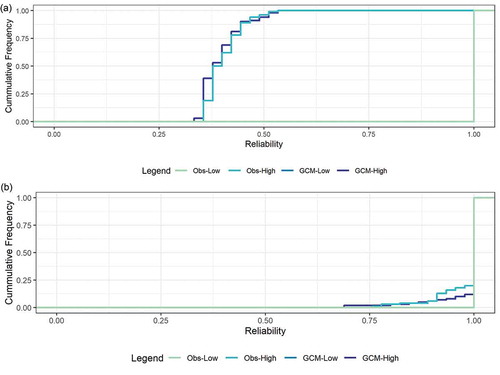
Figure 7 shows the cumulative distribution function (CDF) of water supply reliability for each streamflow and growth scenario combination for both models under BAU. As anticipated, system reliability is greater for the low-growth scenarios than the high-growth scenarios, regardless of the streamflow scenario. Reliability is near even between the observed climate regime and the downscaled GCM projections. Additionally, the endogenous model has higher levels of reliability than the exogenous mode for each scenario.

Figure 7. CDF of reliability for the BAU case for (a) the exogenous water use model, and (b) the endogenous water use model

4.3 Alternatives analysis

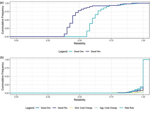
Results for the alternatives analysis are presented from only one scenario, downscaled GCM projected streamflow and high growth, for brevity. Figure 8 presents the CDF plots for both models for the alternatives defined in Section 3.2. The exogenous water use model is, by its nature, incompatible with demand-side interventions and is run only with the two desalination options. Figure 8(a) shows that the traditional desalination plant has a higher reliability. The endogenous water use model facilitates testing of demand-side responses. Reliability results from the endogenous water use model demonstrate that all options outperform BAU, but the aggressive code changes are the most effective, followed closely by moderate code changes (Fig. 8(b)). The rate rule results in the lowest reliability.

Figure 8. CDF of reliability for the response cases for (a) the exogenous water use model, and (b) the endogenous water use model

A review of the water stress heat map (Fig. 9) illuminates differences in both timing and magnitude of water stress across models, and between BAU and active response. The top row of Fig. 9 displays WaSSI heat map results for the exogenous model with (a) BAU and (b) active response. Early periods of these two simulations display similar patterns but they diverge as water stress levels rise, triggering the implementation of desalination projects. Without intervention WaSSI values as high as 1.5 are observed, indicating that demand is 50% higher than available supply. The bottom row of Fig. 9 displays WaSSI values for each year of the simulations with the endogenous model. In both (c) BAU and (d) response cases, WaSSI values are much lower, not rising above 1. Comparing the BAU and responses cases we see a similar phenomenon, where the first half of the two simulations displays a similar pattern, but then they diverge as water stress rises, triggering intervention.

Figure 9. Heat map illustrating the evolution of water stress over time across many model runs using the high population growth and downscaled projected streamflow for the following: (a) BAU with the exogenous model; (b) desalination construction with the exogenous model; (c) BAU with the endogenous model; and (d) demand- and supply-side responses with the endogenous model

5 Discussion

This paper demonstrates the feasibility of including water use as an endogenous variable in a water supply planning model and compares the impact of this approach to the traditional water use scenarios. Accomplishing this required the development of a new module of water salience and the integration of water supply, usage and salience modules.

The threshold-based water salience function fits the timing of increases in the media coverage of water issues well (Fig. 6, Table 3). This indicates both that there is a relationship between water supply and salience (as measured by media coverage) and that the normalized distance from operational thresholds is a reasonable way to represent this relationship. The salience module developed here is specific to the physical and institutional structure of the Las Vegas water supply system. This relationship may shift with time, as demonstrated by this case. While the threshold-based salience function is found to fit the data well throughout the study period, system thresholds changed as new Colorado River agreements were negotiated (Department of the Interior 2001, 2007). Further, shifts in cultural attitudes could prompt changing reactions to similar events (Caldas et al. 2015). In the future, cross-case comparison is recommended to gain greater insight into these temporal changes as well as variation in this relationship across cases. Nonetheless, the water salience module in its current form serves as a novel tool for exploring feedback between supply and demand.

The reservoir operations, banked groundwater, water use and water salience models were combined to create a model of the integrated water supply system. In integrated systems models, errors and uncertainties from one module affect performance in the rest of the model (Refsgaard et al. 2007). This model is unfortunately no exception (Fig. 6, Table 4). Ability to replicate patterns in historical data decreased for per capita water use, water salience and banked groundwater. This is likely because these three modules are strongly coupled, and errors in one module propagate across the other two. The ability to replicate Lake Mead reservoir levels was relatively unaffected, likely because exogenous variables such as streamflow and upstream water usage have a large influence on reservoir levels. Taken as a whole, model performance, while lower than expected for a hydrological model, is deemed reasonable for a socio-hydrological model where error can propagate across subsystems. While not all sociohydrological models have published performance metrics (e.g. Elshafei et al. 2014, Yu et al. 2017), the model performance shown here meets or exceeds the performance of recently published models in this area (e.g. Chen et al. 2016, Roobavannan et al. 2017, Li et al. 2019). For example, Li et al. (2019) reports NSE values for reservoir storage of 0.59 and 0.46, and for groundwater levels of 0.82 and 0.35, for the calibration and validation periods, respectively.

Modeled per capita water use is overestimated during the first half of the study period and underestimated for the second half; these errors likely result from errors in the modeled salience (Fig. 6(a)). However, the accuracy is reasonable for the present purpose: to project system performance across a range of possible futures and compare the relative performance of different alternatives for action. The errors in modeled Lake Mead levels, while small, occur at a time when reservoir levels are approaching critical thresholds (Fig. 6(b)). This therefore impacts the modeled salience. Modeled salience matches the timing but not the magnitudes in the observed data (Fig. 6(c)). This is acceptable because absolute magnitudes in the data have little real-world value; it is the timing and the relative magnitude of salience peaks that is important for understanding how public attention to water issues changes. Therefore, if the parameter connecting salience to demand response, α, is estimated jointly with the salience parameters, the lack of correspondence to salience data magnitudes does not present a problem. Banked groundwater is notably overestimated near the end of the simulation (Fig. 6(d)). This is likely due to the underestimation of demand. With underestimated demand there is excess water available for banking.

Water supply system performance is tested across four scenarios, assuming BAU, using both the endogenous and exogenous water use models. Across both models the difference in system reliability between observed resampled and downscaled streamflow scenarios was lower than expected. This is likely because while overall the streamflow declines under the downscaled GCM projected scenario, the higher variability increases the chance of extreme high flows which refill reservoirs. Further, reliability is lower overall using the exogenous water use model because it incorporates no demand response to water stress events (Fig. 7). Many of the high-growth endogenous model runs show the highest levels of water stress in the middle of the study period, particularly for the observed streamflow scenario. This is because falling reservoir levels trigger increased attention and a conservation response.

The ability of the two models to simulate potential responses to changes in streamflow and demographics was then assessed. The downscaled streamflow high-growth scenario was selected to display and discuss differences across options and models. Both models demonstrate that the addition of desalination increases reliability (Fig. 8) and reduces water stress (Fig. 9), but again the endogenous water use model results show higher levels of reliability than the exogenous water use model. The difference in the gap between the reliability of the flexible and traditional desalination implementation schemes across the two models is notable (Fig. 8). Flexible approaches to implementation decrease the buffer between supply and demand because a portion of capacity is delayed until it is needed to decrease costs and utilize the best available technology when it is needed. The results of the exogenous water use model demonstrate this effect. However, the endogenous water use model results show that the flexible approach has higher reliability. This is because the short-term increase in water stress that occurs under the flexible implementation alternative triggers a conservation response that lowers water use, mitigating the primary risk of flexible design (AlMisnad et al. 2017, Turlington et al. 2017). This observation highlights the importance of modeling water use as an endogenous variable in the model. This model structure allows realistic simulation of reduction of water use in response to water stress.

The demand-side options can only be tested in the endogenous water use model, which is one clear advantage over the water use scenarios. The effectiveness of the code change option is tied to the rate of population growth, so its utility in the high-growth scenario is unsurprising. However, while it may not be as effective in a low-growth future, it is a relatively low-cost and low-regret option. The rate change rule, while not as effective as code changes, increased reliability compared to the BAU case (Fig. 8).

As seen in the model results, the exogenous water use model projects lower levels of reliability and higher levels of water stress. Given the critical nature of water supply, a conservative approach that errs on the side of overprediction could be appealing (Whitman 1932). However, it is also important to consider the costs of overinvesting in water supply capacity. First, there is the financial cost of investing in capacity that is not needed, such as the desalination plants constructed during Australia’s Millennium Drought which are now considered stranded assets (Turner et al. 2016). However, excess capacity also creates a financial incentive for utilities to encourage water use and limit conservation in order to pay off the debt acquired. This highlights the importance of understanding the range of water usage change under different scenarios and assumptions. The endogenous water use model adds to the suite of tools available for water utilities to use to understand this range. Garcia et al. (2019) found the relationship between water utility financial stressors and policy change to be inconsistent across cases. However, the issues of costs and financial incentives deserve greater interrogation in future research.

The endogenous water use model enables the joint evaluation of demand management and water supply augmentation, and the identification of trade-offs and synergies between the two types of strategies. However, there are limitations to the model in its current form. As described above, the water salience function is based on a single case and on a limited historical period. As this period included an extreme drought, it could overestimate future response. However, using the exogenous and endogenous models in concert addresses this limitation by projecting a range of futures from no response to an intensive response. An additional gap in the current analysis is that response alternatives are tested individually, and interactions between alternatives are not explored. Therefore, further exploration of the joint implementation of multiple policies is planned.

6 Conclusions

Urban growth, climate change and the associated uncertainties present a significant challenge for urban water utilities. At the same time, competing priorities for public funds require efficient solutions to these challenges. Water utilities must strike a delicate balance between maintaining high levels of system performance in an uncertain future and spending funds prudently. Accounting for the adaptability inherent in water management, and linking this adaptability to biophysical and institutional conditions, enables exploration of the interactions between supply and demand dynamics, and water utility choices, better informing utility decisions.

This paper builds on the observation that water stress can prompt a durable decline in demand and takes a socio-hydrological approach to integrate endogenous water use into a water supply planning model. It demonstrates the feasibility of this approach first by developing and testing a novel model of water salience as a function of proximity to water supply thresholds. Second, it demonstrates the feasibility of linking water supply, water use and water salience modules to account for feedback between these subsystems. Then, by comparing this model to a water use scenario model to assess system performance under a range of future conditions and potential responses, this work illustrates the implications of demand response to water stress for infrastructure investment. This approach can reduce the risk of stranded assets by bringing findings of sociohydrology into the planning process.

Future application of this modeling framework to additional cases will allow researchers to hold some factors constant and to assess whether observed feedback is broadly applicable. This work, however, represents an important step toward integrating the existing adaptability into water planning models. The introduction of endogenous water use in a water supply planning model enables the concurrent evaluation of supply- and demand-side options to maintain reliability in a changing environment. The model comparison demonstrated that explicitly modeling the dynamics of both institutional and biophysical systems enables exploration of the impact of path dependencies not easily identifiable using water use scenarios.

Acknowledgements

We thank Nicole Lise of the LVVWD and Kent Sovocool of the SNWA for their assistance with data collection and for their feedback. We thank Elizabeth Koebele and Galen Treuer for developing the media coding method. Finally, with sadness and gratitude, we would like to dedicate this work to Dr. Kent Portney, who passed away in 2020. As a teacher, mentor and colleague, Kent shaped both this work and our thinking. We miss him greatly.

Disclosure statement

No potential conflict of interest was reported by the authors.

Supplemental material

Supplemental data for this article can be accessed here.

Additional information

Funding

This work was supported by the National Science Foundation [NSF EEC-1444926,NSF-IGERT 0966093].

References

- AlMisnad, A., de Neufville, R., and Garcia, M., 2017. Risk distribution and the adoption of flexibility: desalination expansion in Qatar. In: S. Islam and K. Madani, eds.. Contingent complexity and prospects for water diplomacy: understanding and managing risks and opportunities for an uncertain water future. New York, NY: Anthem Press, 229–251.
- Beck, M.B., 1999. Coping with ever larger problems, models, and data bases. Water Science & Technology, 39(4), 1–11. International Association on Water Quality. doi:10.1016/S0273-1223(99)00048-7
- Bordalo, P., Gennaioli, N., and Shleifer, A., 2012. Salience theory of chocie under risk. The Quarterly Journal of Economics, 127 (3), 1243–1285. doi:10.1093/qje/qjs018.Advance
- Brelsford, C. and Abbott, J.K., 2017. Growing into water conservation? Decomposing the drivers of reduced water consumption in Las Vegas, NV. Ecological Economics, 133, 99–110. The Authors. doi:10.1016/j.ecolecon.2016.10.012
- Brown, C., et al., 2012. Decision scaling: linking bottom-up vulnerability analysis with climate projections in the water sector. Water Resources Research, 48 (9). doi:10.1029/2011WR011212
- Brun, R., Reichert, P., and Ku, H.R., 2001. Practical identi ability analysis of large environmental simulation models. Water Resources Research, 37 (4), 1015–1030. doi:10.1029/2000WR900350
- Caldas, M.M., et al., 2015. Opinion: endogenizing culture in sustainability science research and policy: fig. 1. Proceedings of the National Academy of Sciences, 112 (27), 8157–8159. doi:10.1073/pnas.1510010112
- Chen, X., et al., 2016. From channelization to restoration: sociohydrologic modeling with changing community preferences in the Kissimmee River Basin, Florida. Water Resources Research, 52 (2), 1227–1244. doi:10.1002/2015WR018194
- Christensen, N.S. and Lettenmaier, D.P., 2007. A multimodel ensemble approach to assessment of climate change impacts on the hydrology and water resources of the Colorado River Basin. Hydrology and Earth System Sciences, 11 (4), 1417–1434. doi:10.5194/hess-11-1417-2007
- Cooley, H., et al., 2007. Hidden oasis : water conservation and efficiency in Las Vegas. (I. Hart, Ed.). Pacific Institute. Available from: http://pacinst.org/publication/hidden-oasis-water-conservation-and-efficiency-in-las-vegas/ [Accessed 01 May 2019],
- Coomes, P.A., et al., 2010. North America residential water usage trends since 1992. US EPA, Washington, DC. Available from: http://www.waterrf.org/PublicReportLibrary/4031.pdf [Accessed 01 October 2018].
- Dawadi, S. and Ahmad, S., 2013. Evaluating the impact of demand-side management on water resources under changing climatic conditions and increasing population. Journal of Environmental Management, 114, 261–275. Elsevier Ltd. doi:10.1016/j.jenvman.2012.10.015
- de Neufville, R. and Scholtes, S., 2011. Flexibility in engineering design. Cambridge, MA: MIT Press.
- Department of the Interior, 2001 Record of decision: colorado river iterim surplus guidelines, final environmental impact statement. Washington DC. Available from: https://www.usbr.gov/lc/region/g4000/surplus/surplus_rod_final.pdf [Accessed 01 May 2019].
- Department of the Interior, 2007 Record of decision: Colorado river interim guidelines for lower basin shortages and the coordinated operations of lake Powell and lake mead. Available from: https://www.usbr.gov/lc/region/programs/strategies/RecordofDecision.pdf [Accessed 01 May 2019].
- Dessaint, O. and Matray, A., 2015. Do managers overreact to salient risks? Evidence from hurricane strikes. SSRN Electronic Journal, 1–63. doi:10.2139/ssrn.2358186
- Di Baldassarre, G., et al., 2013. Socio-hydrology: conceptualising human-flood interactions. Hydrology and Earth System Sciences, 17 (8), 3295–3303. doi:10.5194/hess-17-3295-2013
- Di Baldassarre, G., et al., 2018. Water shortages worsened by reservoir effects. Nature Sustainability, 1 (11), 617–622. doi:10.1038/s41893-018-0159-0
- Draper, A.J. and Lund, J.R., 2004. Optimal hedging and carryover storage value. Journal of Water Resources Planning and Management, 130 (1), 83–87. doi:10.1061/(ASCE)0733-9496(2004)130:1(83)
- Dumedah, G., et al., 2010. Selecting model parameter sets from a trade-off surface generated from the non-dominated sorting genetic algorithm-II. Water Resources Management, 24 (15), 4469–4489. doi:10.1007/s11269-010-9668-y
- Elshafei, Y., et al., 2014. A prototype framework for models of socio-hydrology: identification of key feedback loops and parameterisation approach. Hydrology and Earth System Sciences, 18 (6), 2141–2166. doi:10.5194/hess-18-2141-2014
- Farrelly, M. and Brown, R. 2011. Rethinking urban water management: Experimentation as a way forward? Global Environmental Change, 21 (2), 721–732. doi:10.1016/j.gloenvcha.2011.01.007
- Garcia, M., et al., 2019. Towards urban water sustainability: analyzing management transitions in Miami, Las Vegas, and Los Angeles. Global Environmental Change, 58, 101967. doi:10.1016/j.gloenvcha.2019.101967
- Garcia, M. and Islam, S., 2018. The role of external and emergent drivers of water use change in Las Vegas. Urban Water Journal, 15 (9), 888–898. doi:10.1080/1573062X.2019.1581232
- Garcia, M., Portney, K., and Islam, S., 2016. A question driven socio-hydrological modeling process. Hydrology and Earth System Sciences, 20 (1), 73–92. doi:10.5194/hess-20-73-2016
- Garcia, M., Ridolfi, E., and Di Baldassarre, G., 2020. The interplay between reservoir storage and operating rules under evolving conditions. Journal of Hydrology, 590, 125270. doi:10.1016/j.jhydrol.2020.125270
- Gonzales, P. and Ajami, N., 2017. Social and structural patterns of drought-related water conservation and rebound. Water Resources Research, 1–38. doi:10.1002/2017WR021852
- Hand, M.S., et al., 2015. Risk preferences, probability weighting, and strategy tradeoffs in wildfire management. Risk Analysis, 35 (10), 1876–1891. doi:10.1111/risa.12457
- Hawkins, D.M., 2004. The problem of overfitting. Journal of Chemical Information and Computer Sciences, 44 (1), 1–12. doi:10.1021/ci0342472
- Hester, C.M. and Larson, K.L., 2016. Time-series analysis of water demands in three North Carolina cities. Journal of Water Resources Planning and Management, 142(8), 05016005. doi:10.1061/(ASCE)WR.1943-5452.0000659
- Kahneman, D. and Tversky, A., 1979. Prospect theory: an analysis of decision under risk. Econometrica, 47 (2), 263–292. doi:10.2307/1914185
- Kasprzyk, J.R., et al., 2013. Many objective robust decision making for complex environmental systems undergoing change. Environmental Modelling & Software, 42, 55–71. Elsevier Ltd. doi:10.1016/j.envsoft.2012.12.007
- Kumar, P., 2011. Typology of hydrologic predictability. Water Resources Research, 47 (3). doi:10.1029/2010WR009769
- Lempert, R.J. and Groves, D.G., 2010. Identifying and evaluating robust adaptive policy responses to climate change for water management agencies in the American west. Technological Forecasting and Social Change, 77(6), 960–974. Elsevier Inc. doi:10.1016/j.techfore.2010.04.007
- Li, B., Sivapalan, M., and Xu, X., 2019. Exploration of Beijing’ s water sustainability challenges and solution spaces from a socio-hydrologic perspective. Water Resources Research. 3. doi:10.1029/2018WR023816
- Mayer, P., et al., 2004 Tampa water department residential water conservation study: the impacts of high efficiency plumbing fixture retrofits in single-family homes. Available from: https://www.cuwcc.org/Portals/0/Document-Library/Resources/Water-Efficient-*Product-Information/End-Use-Studies-Multiple-Technologies/Tampa-Residential-Water-Conservation-Final-Report.pdf [Accessed 30 November 2020].
- Mersmann, O., et al., 2014. Multiple criteria optimization algorithms and related functions description. Available from http://git.p-value.net/p/mco.git.LazyData [Accessed 01 May 2019].
- Mersmann, O., et al., 2020 mco: multiple criteria optimization algorithms and related functions. Available from: https://cran.r-project.org/web/packages/mco/mco.pdf [Accessed 01 May 2019].
- Milly, P.C.D., et al., 2008. Stationarity is dead: whither water management? Science, 319 (5863), 573–574. doi:10.1126/science.1151915
- Mini, C., Hogue, T.S., and Pincetl, S., 2015. The effectiveness of water conservation measures on summer residential water use in Los Angeles, California. Resources, Conservation and Recycling, 94, 136–145. Elsevier B.V. doi:10.1016/j.resconrec.2014.10.005
- Montanari, A., et al., 2013. “Panta Rhei—everything flows”: change in hydrology and society—the IAHS scientific decade 2013–2022. Hydrological Sciences Journal, 58 (6), 1256–1275. doi:10.1080/02626667.2013.809088
- Moriasi, D.N., et al., 2015. Hydrologic and water quality models: performance measures and evaluation criteria. Transactions of the ASABE, 58 (6), 1763–1785. doi:10.13031/trans.58.10715
- Mostafaie, A., et al., 2018. Comparing multi-objective optimization techniques to calibrate a conceptual hydrological model using in situ runoff and daily GRACE data. Computational Geosciences, 22 (3), 789–814. doi:10.1007/s10596-018-9726-8
- Mulroy, P., 2008. Beyond the divisions: a compact that unites. Journal of Land, Resources Environmental Law, 28 (1), 105–117.
- Ott Verburg, K., 2010. The Colorado River documents, 2008. Upper Colorado Region, USA: Bureau of Reclamation, Government Printing Office.
- Peng, T., et al., 2018. Modeling and combined application of orthogonal chaotic NSGA-II and improved TOPSIS to optimize a conceptual hydrological model. Water Resources Management, 32(11), 3781–3799. Water Resources Management. doi:10.1007/s11269-018-2019-0
- Quesnel, K.J. and Ajami, N.K., 2017. Changes in water consumption linked to heavy news media coverage of extreme climatic events. Science Advances, 3 (10), 1–10.
- Refsgaard, J.C., et al., 2007. Uncertainty in the environmental modelling process – a framework and guidance. . Environmental Modelling & Software, 22 (11), 1543–1556. doi:10.1016/j.envsoft.2007.02.004
- Roobavannan, M., et al., 2017. Role of sectoral transformation in the evolution of water management norms in agricultural catchments: a sociohydrologic modeling analysis. Water Resources Research, 53 (10), 8344–8365. doi:10.1002/2017WR020671
- Russell, S. and Fielding, K., 2010. Water demand management research: a psychological perspective. Water Resources Research, 46 (5), 1–12. doi:10.1029/2009WR008408
- Schleich, J. and Hillenbrand, T., 2009. Determinants of residential water demand in Germany. Ecological Economics, 68(6), 1756–1769. Elsevier B.V.. doi:10.1016/j.ecolecon.2008.11.012
- Siriwardene, N.R. and Perera, B.J.C., 2006. Selection of genetic algorithm operators for urban drainage model parameter optimisation. Mathematical and Computer Modelling, 44 (5–6), 415–429. doi:10.1016/j.mcm.2006.01.002
- Sivapalan, M. and Blöschl, G., 2015. Time scale interactions and the coevolution of humans and water. Water Resources Research, 51 (9), 6988–7022. doi:10.1002/2015WR017896
- Sivapalan, M., Savenije, H.H.G., and Blöschl, G., 2012. Socio-hydrology: a new science of people and water. Hydrological Processes, 26 (8), 1270–1276. doi:10.1002/hyp.8426
- SNWA, 1995. Amended Cooperative Agreement. Las Vegas, NV: SNWA.
- SNWA, 1999. Memorandom of understanding regarding the Southern Nevada water authority’s water conservation/efficiency programs 1999–2004. Las Vegas, NV: SNWA.
- SNWA, 2005. Integrated water planning advisory committee recommendations report. Las Vegas, NV: SNWA.
- SNWA, 2009. Water resources management plan. Las Vegas, NV: SNWA.
- SNWA, 2013. Integrated resource planning advisory committee recommendations report, phase I: funding sources. Las Vegas, NV: SNWA. Available from: https://www.snwa.com/assets/pdf/ws_irpac_recommendations_final.pdf.
- SNWA, 2014a Intergrated resource planning advisory committee recommendations report phase II: resources and facilities. Available from https://www.snwa.com/ws/cac_recommendations_phase2.html [Accessed 01 August 2017].
- SNWA, 2014b. Meeting of the integrated resource planning advisory committee meeting summary. Las Vegas, NV: SNWA. Available from: https://www.snwa.com/apps/agenda/snwa/index.cfml [Accessed 01 August 2017].
- SNWA, 2015. Water resource plan. Las Vegas, NV: SNWA. Available from: https://www.snwa.com/ws/resource_plan.html [Accessed 01 August 2017]
- State Government of Victoria, 2015. Victorian desalination plant: costs and payments. Authored and published by the State Government of Victoria, location Victoria, Australia. Available from: https://www.water.vic.gov.au/__data/assets/pdf_file/0013/54202/Fact-sheet-project-costs-March-2015.pdf [Accessed 30 November 2020].
- Thompson, S.E., et al., 2013. Developing predictive insight into changing water systems: use-inspired hydrologic science for the Anthropocene. HESS, 17 (12), 5013–5039. doi:10.5194/hess-17-5013-2013
- Treuer, G., et al., 2017. A narrative method for analyzing transitions in urban water management: the case of the Miami-Dade water and sewer department. Water Resources Research, 53 (1), 891–908. doi:10.1002/2016WR019658
- Turlington, M.W., de Neufville, R., and Garcia, M., 2017. Flexible design of water infrastructure systems. In: S. Islam and K. Madani, eds.. Contingent complexity and prospects for water diplomacy: understanding and managing risks and opportunities for an uncertain water future. New York, NY: Anthem Press; 51–73.
- Turner, A., et al., 2016. Managing drought: learning from Australia. Sydney, Australia: Pacific Institute. Available from: http://pacinst.org/publication/managing-drought-learning-from-australia/
- US Bureau of Reclamation, 1970 Criteria for coordinated long-range operation of Colorado River reservoirs pursuant to the Colorado River Basin project act of September 30,1968 (P. L. 90–537). Available from: https://www.usbr.gov/lc/region/pao/pdfiles/opcriter.pdf [Accessed 01 May 2019].
- US Bureau of Reclamation, 2016. Reservoir data: lake Powell. Water Operation History Data. Available from: https://www.usbr.gov/rsvrWater/HistoricalApp.html
- US Bureau of Reclamation, 2018 Upper and lower basin drought contingency plans 11. Available from: https://www.usbr.gov/dcp/docs/DCP_Agreements_Final_Review_Draft.pdf [Accessed 01 May 2019].
- USBR, 2012a. Colorado River Basin water supply and demand study. Available from: https://www.usbr.gov/lc/region/programs/crbstudy/finalreport/index.html
- USBR, 2012b Colorado River Basin supply and demand study: technical report B - water supply assessment. Available from: http://www.usbr.gov/lc/region/programs/crbstudy/finalreport/index.html [Accessed 01 May 2019].
- USBR, 2012c. Colorado River Basin supply and demand study: technical report B - water supply assessment.
- Vogel, R.M., Yaindl, C., and Walter, M., 2011. Nonstationarity: flood magnification and recurrence reduction factors in the United States. Journal of the American Water Resources Association, 47 (3), 464–474. doi:10.1111/j.1752-1688.2011.00541.x
- Wei, J., Wei, Y., and Western, A., 2017. Evolution of the societal value of water resources for economic development versus environmental sustainability in Australia from 1843 to 2011. Global Environmental Change, 42, 82–92. Elsevier Ltd. doi:10.1016/j.gloenvcha.2016.12.005
- Wentz, E.A. and Gober, P., 2007. Determinants of small-area water consumption for the City of Phoenix, Arizona. Water Resources Management, 21 (11), 1849–1863. doi:10.1007/s11269-006-9133-0
- Whitman, E.B., 1932. Per Capita water consumption. Journal - American Water Works Association, 24 (4), 515–528. doi:10.1002/j.1551-8833.1932.tb18069.x
- Yu, D.J., et al., 2017. Incorporating institutions and collective action into a sociohydrological model of flood resilience. Water Resources Research, 1–18. doi:10.1002/2016WR019746
- Zhang, C., et al., 2017. Exploring the relationships among reliability, resilience, and vulnerability of water supply using many-objective analysis. Journal of Water Resources Planning and Management, 143 (8), 04017044. doi:10.1061/(ASCE)WR.1943-5452.0000787