Modelling surface water dynamics in an Amazonian sub-basin: impacts of hydraulic geometry refinement

ABSTRACT

This study describes the impacts of refinement of hydraulic geometry (HG) relationships in the hydrological MGB model applied to an Amazonian sub-basin (Purus River basin). To this end, HG relationships were developed for the entire basin and for hydrologically homogeneous regions, and their performances were compared with observed data and a global width and depth database. Two simulations were then performed using the MGB model: one using the refined HG relationships and the other using the global width and depth database. The simulated streamflow and water level estimates were compared with observed data. The results showed that HG relationships for the hydrologically homogeneous regions provided better estimates of hydraulic parameters for the basin, with Nash-Sutcliffe efficiency of 0.96 for width and 0.95 for depth, and its use provided an improvement in the performance of the hydrological modelling in some gauge stations, with an increase in the Nash-Sutcliffe efficiency between 18% and 65%.

KEYWORDS:

• fluvial geomorphology
• Purus River basin
• MGB model
• GRWD

Editor A. Castellarin Associate Editor M. Sadegh

1 Introduction

Reliable hydrological streamflow simulations and related processes are vital to support water resource management in relation to water security, natural hazards, navigation, agriculture and energy production. Therefore, better forecasting of the hydrological system can help policy makers and stakeholders make better decisions by promoting actions to reduce risks and impacts on water resources under current and future conditions (Siqueira et al. 2018).

A characteristic of semi-distributed hydrological models, applied at regional or larger scales, is the need to have the cross-section parameters of all channels belonging to the river network in the study domain, which can be obtained from in situ measurements, which are reliable but limited to a small number of locations. As a result, channel cross-section parameters have generally been estimated based on available basin characteristics (such as drainage area and streamflow) using empirical equations, known as hydraulic geometry (HG) relationships (Luo et al. 2017, Fleischmann et al. 2019, Andreadis et al. 2020).

The concept of HG relationships was first introduced by Leopold and Maddock (1953) to describe the dependence of channel dimensions on streamflow in specific river basins. Based on a study of river gauge stations records in the United States, they expressed the relationship between average annual streamflow and river channel width and depth, for different regions of the country, in terms of simple power functions.

Since the use of discharge as an independent variable limits the applicability of HG equations to gauged stream reaches, Dunne and Leopold (1978) introduced the use of drainage area as a substitute for discharge. Acquiring complete channel geometry measurements can be time consuming and cost prohibitive, while bankfull HG relationships can provide the channel dimensions by using only the drainage area, which can be derived from readily available Digital Elevation Models (Bieger et al. 2015).

Some modelling studies in the last few years employed HG relationships for regional- and continental-scale basins (Coe et al. 2008, Paiva et al. 2011, 2013, Pontes et al. 2017, Siqueira et al. 2018, Fleischmann et al. 2019). For simplicity, these studies considered that river cross-sections are rectangular and used measured river width and depth data at various locations associated with different drainage area values. The approximation of rectangular cross sections has been considered satisfactory to estimate water levels, and recent studies have shown the capacity of rectangular channels to simulate flooding processes (Paiva et al. 2013, Pontes et al. 2017, Grimaldi et al. 2018, Siqueira et al. 2018, Fleischmann et al. 2019).

Among the examples of HG relationships developed for river basins of regional/continental scales are those developed by Bieger et al. (2015), for the physiographic divisions of the United States; by Paiva et al. (2013), for six of the largest Amazonian sub-basins; by Pontes et al. (2017), for the Plate River basin, in South America; by Fagundes et al. (2017), for the Doce River basin, in Brazil; by Morel et al. (2020), for stream reaches in France and New Zealand; and by Adeyemi et al. (2020) for the Upper Ogun River Basin, in Southwestern Nigeria.

Regarding HG relationships on a global scale, the most relevant example is the database developed by Andreadis et al. (2013). They developed a worldwide database of channel widths and depths, called the Simple Global River Bankfull Width and Depth Database (GRWD) (http://gaia.geosci.unc.edu/rivers/), based on the HydroSHEDS hydrography data set and streamflow data from the Global Runoff Data Center (GRDC).

In most of the mentioned studies, the cross-section parameters of the channels were estimated using a set of HG relationships and corresponding parameters that represent the average characteristics of a basin, region or even continent. Thus, for different sub-basins, the cross-sectional parameters of the channels derived from the same equations and parameters can contain biases of various magnitudes (Luo et al. 2017).

Taking into account that the results of hydrodynamic modelling in several studies demonstrated sensitivity to cross-section parameters and that the largest gain towards locally relevant water levels would be obtained by using better cross-section parameters, with more correct estimates of bankfull width and depth values (Paiva et al. 2013, Luo et al. 2017, Siqueira et al. 2018, Fleischmann et al. 2019, Andreadis et al. 2020), it is hypothesized that the improvement of the flood dynamic representation in hydrodynamic modelling can be done by refining the HG relationships discretized for hydrologically homogeneous regions.

The scarcity of cross-sectional data measured in situ and the absence of more refined representative hydraulic geometry relationships could have important impacts on modelling surface hydrology in the Amazon region. Therefore, this study aims to evaluate the impact of improving the representation of river channel bankfull widths and depths by refining hydraulic geometry (HG) relationships in hydrological-hydrodynamic modelling in an Amazonian subbasin using the MGB model (“Modelo Hidrológico de Grandes Bacias”), calibrated for all of South America (MGB SA) (Siqueira et al. 2018). The model performance was evaluated against gauged streamflow and water level data and the results were also compared with those using more general global width and depth databases.

2 Material and methods

2.1 Study area

The study area of this work consists of the Purus River basin, located primarily in the south-western depression of the Amazon region, with a total area of approximately 375,458 km² and elevations varying between 9 and 600 m (Fig. 1). The Purus River is one of the main tributaries of the Solimões/Amazonas system, being one of the longest rivers in South America, rising in the lowlands of eastern Peru and flowing approximately 3,380 km before encountering the Solimões River in northwest Brazil (Ríos-Villamizar et al. 2017).

Figure 1. Purus river basin

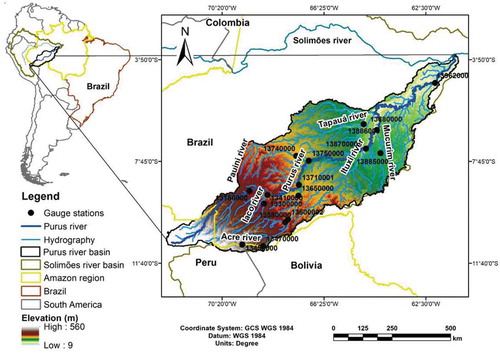
The Purus River basin has a drainage network with a dendritic pattern, without strong geological controls (Latuf and Amaral 2016). Due to the great distances covered and the extensive flood plains in the medium/low Purus, the propagation time of the flood waves is very high, reaching more than 30 days. This factor contributes strongly to the attenuation of hydrographs (Paiva 2009).

In addition, due to the characteristics of the relief in Central Amazonia, the backwater effects regulate part of the hydraulic behaviour of the Purus River, causing a 3 m difference between the water levels in the descent and ascent of the hydrograph (Meade et al. 1991). Normally, the high flow season in the basin occurs from January to June, while the low flow season occurs from July to December. The average long-term flow near the mouth of the Purus River is 15,285 m³/s at the Arumã-Jusante (code: 13962000) river gauge station from the Brazilian National Water Agency (ANA), with a drainage area of 366,384 km².

The basin’s climate, according to the Köppen climate classification, is Humid Equatorial (Af), characterized by a minimum monthly rainfall of 60 mm and an average temperature ranging between 26°C and 28°C (Peel et al. 2007). Two seasonal periods are defined by the rains in the Purus River basin: the dry season, from April to September, and the rainy season, from October to March. Precipitation reaches its peak from December to February (average of 300 mm) and its lowest from May to August (average of 60 mm) (Dalagnol et al. 2017).

2.2 Channel geomorphology

To obtain bankfull width and depth values, cross-section data from ANA gauge stations were used (http://www.snirh.gov.br/hidroweb). Currently, the operation of ANA’s fluviometric network in the Amazon region has a low density of stations, with measurements spaced every three months. Thus, it was possible to work with cross-section historical series from 16 gauge stations in the Purus River basin (Fig. 1), varying between 1996 and 2017, totalling 148 hydraulic geometry observations corresponding to drainage areas ranging from 5,789 to 366,384 km².

To determine bankfull width and depth, the cross-sections were represented by equivalent units characterized by the bankfull width (W) and an equivalent bankfull depth (D), where the cross-section area is conserved. Then, the mean values of the entire historical series of W and D were calculated for each gauge station analysed (Table 1).

Table 1. Bankfull width (W) and depth (D) obtained for the cross-sections of river gauge stations located in the Purus River basin

Gauge station	Name	River	Lat	Long	A (km^2)	W (m)	D (m)
13180000	Manoel Urbano	Purus	−8.89	−69.28	32,714	214.6	7.5
13300000	Seringal São José	Iaco	−9.37	−68.72	11,264	170.1	6.7
13410000	Seringal da Caridade	Purus	−9.04	−68.59	63,108	261.1	12.9
13450000	Assis Brasil	Acre	−10.95	−69.56	3,722	86.7	4.7
13470000	Brasiléia	Acre	−11.01	−68.75	7,035	106.7	6.6
13580000	Fazenda Santo Afonso	Branco	−10.09	−67.90	6,400	80.5	6.2
13600002	Rio Branco	Acre	−9.98	−67.80	23,484	130.3	10.5
13650000	Floriano Peixoto	Acre	−9.07	−67.40	34,699	210.7	9.7
13,710,001	Valparaíso-Montante	Purus	−8.65	−67.38	105,476	350.4	12.2
13740000	Fazenda Borangaba	Pauini	−7.54	−67.48	23,957	146.4	9.9
13750000	Seringal Fortaleza	Purus	−7.72	−67.00	154,242	379.5	16.0
13870000	Lábrea	Purus	−7.26	−64.80	226,939	471.0	16.7
13880000	Canutama	Purus	−6.54	−64.38	236,373	478.6	17.7
13885000	Cristo	Mucuim	−7.43	−64.24	5,789	171.1	5.6
13886000	Bacaba	Tapaua	−6.31	−64.89	38,228	292.8	5.9
13962000	Arumã-Jusante	Purus	−4.73	−62.14	366,384	726.1	24.0

where Lat is the latitude; Long is the longitude; A is the drainage area; W is the bankfull width; and D is the bankfull depth.

2.3 Hydraulic geometry relationships

Using exponential regression, general relationships for the entire Purus River basin, using data from all gauge stations, were developed. Exponential regression has been defined in several studies as the one that best represents the relationship between channel parameters and drainage area, and its use was recommended by several authors, including Andreadis et al. (2013), Bieger et al. (2015), Frasson et al. (2019) and Paiva et al. (2013).

These equations were obtained through a statistical relationship for bankfull width and depth as a function of the upstream drainage area of each gauge station, and the quality of the fit was analysed by the coefficient of determination (r²). The relationships between the parameters were adjusted in the software R 3.3.1® based on Equations 1(1) $\mathrm{D}=\mathrm{a}\times {\mathrm{A}}^{\mathrm{b}}$(1) and 2(2) $\mathrm{W}={\mathrm{a}}^{\prime }\times {\mathrm{A}}^{{\mathrm{b}}^{\prime }}$(2) (Dunne and Leopold 1978), using the Gauss-Newton algorithm, which is an iterative method regularly used to solve nonlinear least-squares problems.

(1) $\mathrm{D}=\mathrm{a}\times {\mathrm{A}}^{\mathrm{b}}$(1)

(2) $\mathrm{W}={\mathrm{a}}^{\prime }\times {\mathrm{A}}^{{\mathrm{b}}^{\prime }}$(2)

where W is the width (m); D is the depth (m); A is the drainage area (km²); and a, b, a’ and b’ are regression parameters.

The equations were applied to the drainage areas of each gauge station, and the estimated bankfull width and depth values were compared with the observed data using some efficiency metrics commonly applied in hydrological studies: the coefficient of determination (r²), the root-mean-square error (RMSE), the mean absolute error (MAE), the mean bias error (MBE), the Nash-Sutcliffe efficiency (NSE), and the Log-transformed Nash-Sutcliffe efficiency (NSE_log). The metrics equations and their range and optimal values are shown in Table 2.

Table 2. Efficiency metrics used in this study

Metric	Abbreviation	Assessment	Equation	Range	Optimal Value
Coefficient of Determination	r^2	Linear correlation		0.0 to 1.0	1.0
Root Mean Square Error	RMSE	Deviation of predicted values	$\mathrm{R}\mathrm{M}\mathrm{S}\mathrm{E}=\sqrt{\frac{1}{\mathrm{n}}\sum _{\mathrm{i}=1}^{\mathrm{n}}{\left({\mathrm{P}}_{\mathrm{i}}-{\mathrm{O}}_{\mathrm{i}}\right)}^2}$	0.0 to ∞	0.0
Mean Absolute Error	MAE	Deviation of predicted values	$\mathrm{M}\mathrm{A}\mathrm{E}=\frac{1}{\mathrm{n}}\sum _{\mathrm{i}=1}^{\mathrm{n}}\left|{\mathrm{P}}_{\mathrm{i}}-{\mathrm{O}}_{\mathrm{i}}\right|$	0.0 to ∞	0.0
Mean Bias Error	MBE	Deviation of predicted values	$\mathrm{M}\mathrm{B}\mathrm{E}=\frac{1}{\mathrm{n}}\sum _{\mathrm{i}=1}^{\mathrm{n}}\left({\mathrm{P}}_{\mathrm{i}}-{\mathrm{O}}_{\mathrm{i}}\right)$	-∞ to ∞	0.0
Nash-Sutcliffe efficiency	NSE	Agreement for high values	$\mathrm{N}\mathrm{S}\mathrm{E}=1-\frac{{\sum }_{\mathrm{i}=\mathrm{i}}^{\mathrm{n}}{\left({\mathrm{O}}_{\mathrm{i}}-{\mathrm{P}}_{\mathrm{i}}\right)}^2}{{\sum }_{\mathrm{i}=\mathrm{i}}^{\mathrm{n}}{\left({\mathrm{O}}_{\mathrm{i}}-\bar{\mathrm{O}}\right)}^2}$	-∞ to 1.0	1.0
Log-transformed Nash-Sutcliffe efficiency	NSElog	Agreement for low values	$\mathrm{N}\mathrm{S}{\mathrm{E}}_{\mathrm{l}\mathrm{o}\mathrm{g}}=1-\frac{{\sum }_{\mathrm{i}=1}^{\mathrm{n}}{\left(\mathrm{l}\mathrm{o}\mathrm{g}{\mathrm{O}}_{\mathrm{i}}-\mathrm{l}\mathrm{o}\mathrm{g}{\mathrm{P}}_{\mathrm{i}}\right)}^2}{{\sum }_{\mathrm{i}=1}^{\mathrm{n}}{\left(\mathrm{l}\mathrm{o}\mathrm{g}{\mathrm{O}}_{\mathrm{i}}-\mathrm{l}\mathrm{o}\mathrm{g}\bar{\mathrm{O}}\right)}^2}$	-∞ to 1.0	1.0
Overall BIAS (%)	BIAS	Under- and overestimation	$\mathrm{B}\mathrm{I}\mathrm{A}\mathrm{S}=\left(\frac{{\sum }_{\mathrm{i}=\mathrm{i}}^{\mathrm{n}}{\mathrm{P}}_{\mathrm{i}}-{\sum }_{\mathrm{i}=\mathrm{i}}^{\mathrm{n}}{\mathrm{O}}_{\mathrm{i}}}{{\sum }_{\mathrm{i}=\mathrm{i}}^{\mathrm{n}}{\mathrm{O}}_{\mathrm{i}}}\right)\times 100$	-∞ to ∞	0.0
Kling-Gupta efficiency	KGE	Overall performance	$\mathrm{K}\mathrm{G}\mathrm{E}=1-\sqrt{{\left(\mathrm{r}-1\right)}^2+{\left(\frac{{\sigma }_{\mathrm{p}}}{{\sigma }_{\mathrm{o}}}-1\right)}^2+{\left(\frac{\bar{\mathrm{P}}}{\bar{\mathrm{O}}-1}\right)}^2}$	-∞ to 1.0	1.0
BIAS in standard deviation (%)	σBIAS	Under- and overestimation	$\sigma \mathrm{B}\mathrm{I}\mathrm{A}\mathrm{S}=\left(\frac{{\sigma }_{\mathrm{p}}-{\sigma }_{\mathrm{o}}}{{\sigma }_{\mathrm{o}}}\right)\times 100$	-∞ to ∞	0.0

where n is the number of observations; P_i is the simulated variable; O_i is the observed variable; is the mean of the simulated variable; is the mean of the observed variable; σ_p is the standard deviation of the simulated variable; and σ_o is the standard deviation of the observed variable.

2.4 Hydrologically homogeneous regions (HHRs)

For grouping gauge stations into hydrologically homogeneous regions based on channel hydraulic geometries, the geographical convenience method was used. This method of identifying homogeneous regions is based on the subjective and/or convenient grouping of gauge stations, usually contiguous, in administrative areas or in areas previously defined according to arbitrary limits (Naghettini and Pinto 2007).

For its application, the gauge stations were initially randomly partitioned into different groups, with at least four stations. For each group, HG relationships were obtained through exponential regression between the geomorphological variables and the drainage area, based on Equations 1(1) $\mathrm{D}=\mathrm{a}\times {\mathrm{A}}^{\mathrm{b}}$(1) and 2(2) $\mathrm{W}={\mathrm{a}}^{\prime }\times {\mathrm{A}}^{{\mathrm{b}}^{\prime }}$(2) . This procedure was then repeated several times for different combinations of stations, also varying the number of clusters.

Finally, the coefficients of regression (r²) were analysed, in addition to the root-mean-square error (RMSE) and the Nash-Sutcliffe efficiency index (NSE) (Table 2), between the observed depths and widths and those estimated by the exponential models that best fit the distribution of geomorphological variables. Next, it was assumed that the combination of stations that had the best fit constituted a hydrologically homogeneous region. The HHR calculations using the geographical convenience method were performed using the software R 3.3.1® (R Core Team 2014).

The equations developed for the HHRs were also applied to the drainage areas of each gauge station, and the estimated bankfull width and depth values were compared with the observed data using efficiency metrics. To evaluate whether the use of refined HG relationships for large river basins improves the representation of the geomorphological characteristics of river channels, the same efficiency metrics were calculated for the GRWD data and then compared with those obtained for the HG relationships.

2.5 Hydrologic-hydrodynamic modelling with MGB SA

The MGB, Modelo Hidrológico de Grandes Bacias (Large-Scale Hydrological Model), is a conceptual, semi distributed, large-scale hydrological model first presented by Collischonn (2001) (https://www.ufrgs.br/hge/mgb). For this study, we used the continental-scale hydrodynamic model version from Siqueira et al. (2018) (MGB SA) that was developed to perform an integrated, multi-basin simulation over the whole South American domain.

The choice of MGB for this study was motivated by several past applications in Brazil and South America, which encompassed rapid responses to markedly seasonal and often slow response basins (e.g. Bravo et al. 2012, Paiva et al. 2013, Siqueira et al. 2016, Fan et al. 2016, Pontes et al. 2017).

The MGB SA uses a fixed-length, vector-based discretization to divide basins into unit-catchments with equal river flow distances (Δx = 15 km), and each river has an associated floodplain profile computed using the height above nearest drainage (HAND) approach (Rennó et al. 2008). Unit catchments are further divided into hydrological response units (HRUs) categorized based on soil type and land use, and for each HRU, the water and energy budget are calculated through the soil–vegetation system.

Surface, subsurface and groundwater flows generated from the water balance are propagated to the main channel of the unit-catchment using linear reservoirs, while streamflow routing in river networks is computed using the local explicit inertial approximation of Saint-Venant equations (Pontes et al. 2017). The streamflow is computed by multiplying the lateral inflow variable by the bankfull channel width (W), which means that the effective flow area is limited by the rectangular channel geometry. Similar to Yamazaki et al. (2011) and Luo et al. (2017), the water mass is instantaneously exchanged between the channel and floodplain when the bankfull depth (D) is exceeded, whereas the water surface elevation of both storages is assumed to be equal within a given unit-catchment.

The model was manually calibrated for the period 1990–2010 using hundreds of gauge stations (>10,000 km²) from several hydrological institutions and was validated using products from multiple sources, including remote sensing data (e.g. terrestrial water storage, evapotranspiration and water levels). For additional details about the MGB SA model, the reader is referred to Siqueira et al. (2018).

The MGB SA model was used to simulate the water dynamics in the Purus River basin. Two hydrological variables were assessed for the period from 1990 to 2010: daily streamflow and daily water level. To investigate the role of refinement of HG relationships in the quality of streamflow and water level modelling in the studied basin, two simulations were performed with different geomorphological databases, width and depth values obtained through the HG relationships with better performance in the basin and the GRWD.

The simulated streamflow and water level values were compared with observed data from gauge stations from 1990 to 2010. The efficiency metrics considered to compare the simulated and observed streamflow values were the coefficient of determination (r²), the Nash-Sutcliffe efficiency (NSE), the Log-transformed Nash-Sutcliffe efficiency (NSE_log), the Overall BIAS (BIAS) and the Kling-Gupta efficiency (KGE), as shown in Table 2.

For the goodness-of-fit assessment of hydrological models, some evaluation criteria for recommended statistical performance measures have been suggested in the literature. Based on the performance of the watershed- and field-scale models, Moriasi et al. (2015) proposes that the NSE should be considered as “not satisfactory”, if NSE ≤ 0.50; “satisfactory”, if 0.50 < NSE ≤ 0.70; “good”, if 0.70 < NSE ≤ 0.80; and “very good”, if NSE > 0.8. Various authors also use positive KGE values as indicative of “good” model simulations (Siqueira et al. 2018, Sutanudjaja et al. 2018, Knoben et al. 2018), even though Knoben et al. (2019) suggest that model simulations with −0.41 < KGE < 1 could be considered with reasonable performance.

For a proper comparison of the observed and simulated water levels, these were first converted to anomalies (subtracting their long-term mean) to maintain the values with the same reference, according to Equation 3(3) ${\mathrm{h}}_{\mathrm{n}\mathrm{e}\mathrm{w}}={\mathrm{h}}_{\mathrm{m}}-\overline{{\mathrm{h}}_{\mathrm{m}}}$(3) (Siqueira et al. 2018).

(3) ${\mathrm{h}}_{\mathrm{n}\mathrm{e}\mathrm{w}}={\mathrm{h}}_{\mathrm{m}}-\overline{{\mathrm{h}}_{\mathrm{m}}}$(3)

where h_new is the water level anomaly (m); h_m is the water level (m); and $\overline{{\mathrm{h}}_{\mathrm{m}}}$ is the long-term mean water level (m).

The efficiency metrics considered to compare the simulated and observed anomalies were the coefficient of determination (r²), the Nash-Sutcliffe efficiency (NSE) and the BIAS in standard deviation (σBIAS), as shown in Table 2.

3 Results and discussion

3.1 Hydrologically homogeneous regions and hydraulic geometry relationships

The geographical convenience method allowed the division of the Purus River basin into two hydrologically homogeneous regions (Fig. 2) so that the HG relationships were improved in relation to the equations for the entire basin, as shown in Table 3, which presents the HG relationships obtained for the entire basin using the 16 stations analysed and for the homogeneous regions defined by the geographical convenience method.

Table 3. Hydraulic geometry relationships obtained for the Purus River basin

Entire basin
	No. of stations	Depth (D)	r^2	Width (W)	r^2
Purus river basin	16	D = 0.2643⋅A^0.3430	0.91	W = 1.5996⋅A^0.4676	0.93
Hydrologically homogeneous regions
HHR 1	12	D = 0.5147⋅A^0.2830	0.92	W = 2.405⋅A^0.4404	0.97
HHR 2	4	D = 0.0362⋅A^0.5044	0.96	W = 5.7287⋅A^0.3708	0.93

Figure 2. Hydrologically homogeneous regions (HHR) obtained for the Purus River basin

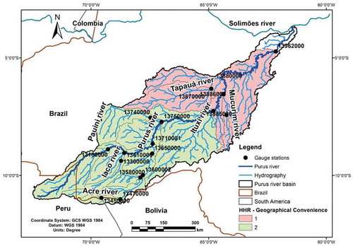
HHR 1, located in the south of the basin, has a set of five stations located on the Purus River itself and seven stations located on affluent rivers. The drainage areas upstream of the gauge stations vary between 3,722 and 226,938 km², the channel depths between 4 and 17 meters and the channel widths between 86 and 471 meters.

HHR 2, located north of the basin, has two stations located on the Purus River itself and two stations located on affluent rivers. The drainage areas upstream of the gauge stations vary between 5,789 and 366,384 km², the channel depths between 5 and 24 meters and the channel widths between 171 and 726 meters.

This division of the basin into an upper and a lower region can be explained, mainly, by the configuration of the relief and the different rainfall and flow regimes that occur in the two regions (Filizola et al. 2011). An important factor in the definition of the cross sections is the existence of flood plains in the lower part of the Purus River basin, while the upstream river cross sections are more well defined. Additionally, the highest precipitation values are found in the lower Purus section, while in the medium Purus, there is a transition from the higher rainfall indexes in the lower Purus to more moderate rainfall in the upper Purus (Espinoza Villar et al. 2009).

Filizola et al. (2011), analysing the streamflow regime in the Purus River basin, concluded that there is an increase in the order of magnitude of the streamflow between the Lábrea (13870000) and Arumã Jusante (13962000) gauge stations. These stations limit HHR 2, which shows that streamflow is a characteristic that also strongly influences the grouping of stations. Another important point highlighted by Filizola et al. (2011) is that the Purus River basin has a very complex mouth as a result of the backwater effect of the Solimões River on the Purus River (Alsdorf et al. 2007). This effect is felt more than 200 km upstream of its mouth and has a great influence on the flow regime of rivers located close to the Purus River mouth.

Table 3 shows that the depth and width HG relationships obtained for the entire Purus River basin showed adjustments with high values of r² of 0.91 and 0.93, respectively. The breakdown of the equations for the HHRs, however, provided an improvement in the adjusted coefficients of the width and depth equations for the homogeneous regions, being more expressive for the depth equation in HHR 2 and for the width equation in HHR 1.

Table 4 presents the efficiency metrics calculated for the results of width and depth obtained by applying the HG relationships generated for the Purus River basin and for the GRWD global data in comparison to the values observed at the locations of the gauge stations. It is noted that the refinement of the equations enabled a better representation of channel geomorphology in the Purus River basin.

Table 4. Efficiency metrics for the comparison between width and depth data obtained by different methods and observed data from gauge stations in the Purus River basin

	RMSE	MAE	MBE	NSE	NSElog
Width
GRWD	150.65	129.93	127.86	0.22	0.44
HG relationship for the entire basin	43.69	34.97	−3.44	0.93	0.87
HG relationships for the HHRs	33.42	24.58	−1.22	0.96	0.95
Depth
GRWD	5.62	4.86	−4.84	−0.13	−0.76
HG relationship for the entire basin	1.63	1.28	−0.06	0.91	0.86
HG relationships for the HHRs	1.24	1.01	−0.07	0.95	0.82

The HG relationships obtained for the HHRs enabled the best agreement of the width and depth estimates with the data observed at the locations of the gauge stations when compared to the global data GRWD. There was mainly an increase in the values of the NSE and NSE_log agreement indices and a reduction in the error indices. The improvement was even more expressive for the depth data, which showed negative values of NSE and NSE_log for the global GRWD data, indicating that the average of the observed data would be a better predictor than this model.

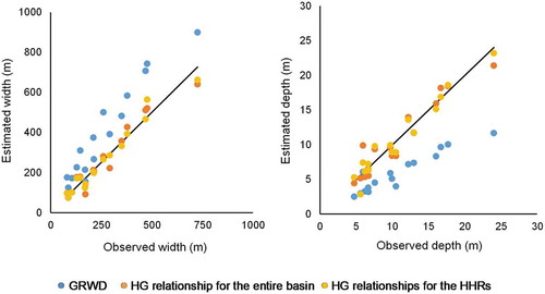
Figure 3 shows the dispersion diagrams between observed and estimated bankfull widths and depths obtained by the different databases. The GRWD data overestimate the widths and underestimate the depths of the channel cross-sections in relation to the observed data, which causes an underestimation of the river cross-sectional areas. Additionally, reaffirming what was seen in Table 4, it can be noted in Fig. 3 that the width and depth values obtained through refined HG relationships are closer to the observed data than the global dataset.

Figure 3. Dispersion diagrams between observed and estimated bankfull widths and depths

3.2 Hydrodynamic modelling with MGB SA

The performance results of the MGB SA model using the GRWD data and the HG relationships obtained for the HRRs are presented in this section. According to the recommendation of Siqueira et al. (2018), values between the ranges of −0.05 to +0.05 for the d_NSE, d_NSE_log, d_KGE differences and values between the −5% to 5% ranges for the d_BIAS and d_ σBIAS differences were considered non-significant.

3.2.1 Streamflow modelling

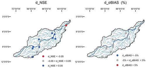
Figure 4 shows the difference between the performances of MGB SA for the streamflow metrics using the GRWD data and the HG relationships for the HHRs of the Purus River basin. It is observed that, using the HG relationships for the HHRs, there was an improvement in the efficiency metrics for some localities, mainly near the mouth of the basin, when compared to the GRWD data.

Figure 4. Difference between the performances of MGB SA for streamflow metrics using GRWD data and using HG relationships for HHRs for the Purus River basin

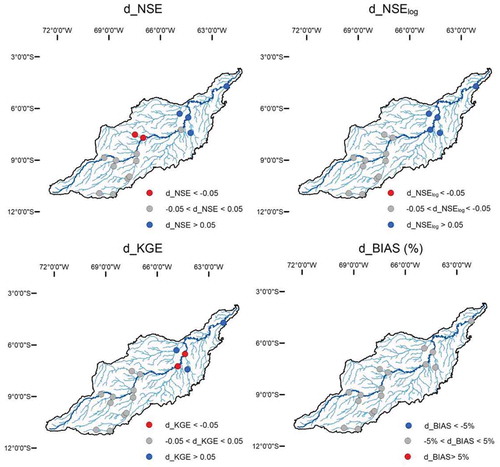
The simulated streamflow values at the locations of Arumã-Jusante (13962000), Bacaba (13886000), Cristo (13885000) and Canutama (13880000) stations showed improvement when compared with the observed data in at least three of the four efficiency metrics analysed (NSE, NSE_log and KGE). Only at the locations of the Seringal Fortaleza (13750000) and Fazenda Borangaba (13740000) stations, in the center of the basin, there was a decrease in the NSE, and for the Canutama and Lábrea stations, there was a decrease in the KGE. At the other stations, there was no significant change in the metrics analysed.

As mentioned earlier, different streamflow regimes occur in the upstream and downstream regions of the Purus River basin. There is an increase in the order of magnitude of the flows between the gauge stations of Lábrea (13870000) and Arumã Jusante (13962000), where there were improvements in the efficiency metrics of the streamflow modelling. Therefore, the simulated streamflow values for the locations of the stations close to the mouth of the basin obtained better performance with the use of HG relationships due to the occurrence of greater flows and, consequently, greater magnitude and frequency of river overflow phenomena in the flood areas. The refinement of the bankfull width and depth data affects the area of the floodplain, resulting in the improvement of the simulated hydrographs.

Table 5 shows the performances of MGB SA using the GRWD data and the HG relationships for some gauge stations that had the performance increase in at least one of the evaluated streamflow metrics in the Purus River basin. As can be seen, the stations of Canutama, Bacaba and Cristo had an increase in the NSE values of 18%, 35% and 65%, respectively, when using HG relationships. According to Moriasi et al. (2015) classification, streamflow modelling went from “unsatisfactory” to “satisfactory” in Canutama, from “satisfactory” to “good” in Bacaba and “unsatisfactory” to good’ in Cristo.

Table 5. Streamflow metrics using GRWD data and using HG relationships for HHRs for the Purus River basin

Gauge station	Name	Hydraulic geometries	NSE	NSElog	KGE	BIAS (%)
13880000	Canutama	GRWD	0.45	0.58	0.66	26.50
		HG relationships	0.53	0.79	0.56	28.30
13870000	Lábrea	GRWD	0.50	0.69	0.59	33.90
		HG relationships	0.48	0.79	0.50	35.30
13886000	Bacaba	GRWD	0.55	0.15	0.65	−0.50
		HG relationships	0.74	0.70	0.87	−1.00
13885000	Cristo	GRWD	0.43	0.25	0.37	−4.30
		HG relationships	0.71	0.79	0.63	−3.90

The NSE_log also increased for all stations presented, having improvement rates of 36%, 14%, 367% and 216% for the Canutama, Lábrea, Bacaba and Cristo stations, respectively. In addition, the KGE values were greater than zero in all simulations, but had an increase of 34% and 70% for the Bacaba and Cristo stations when using HG relationships instead of GRWD data.

Figure 5 presents the observed and simulated hydrographs using the GRWD data and the HG relationships for the gauge stations presented in Table 5. It can be noted that for the analysed stations, there was an improvement in the simulated hydrographs, mainly with regard to the time lag, in which the simulated streamflow values using HG relationships for the HHRs of the Purus River were closer to the observed data compared to the GRWD data.

Figure 5. Comparison between streamflow simulated using geomorphological data from GRWD and from HG relationships with streamflow observed in the gauge stations in the Purus River basin

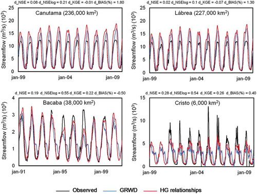
There was also a small improvement in peak flow simulation using HG relationships for HHRs. Faults in river cross-section dimension estimates using less accurate width and depth data, such as GRWD, cause errors in the flood extent and, consequently, in the volume exchanged with the floodplain, causing the model to underestimate streamflow amplitude (Paiva 2012).

It is also noted that even with the improvement in peak flow simulation using HG relationships for HHRs, there is still difficulty in modelling these data, mainly due to the influence of the flooded areas in the calculation of maximum flows, a factor of great relevance in the Amazon basin (Paiva 2012). The model’s bias may also be due to a failure in the calibration of the MGB SA, which was done manually considering a set of parameters of HG relationships developed by Paiva et al. (2011) for the Purus and Juruá river basins.

It is important to mention that the “observed” flow data series are normally used as reliable representations of the “truth” (Getirana 2010). However, there are also uncertainties in these data since they are obtained indirectly through traditional rating curves. These uncertainties are even greater for peak flows, where, in most cases, these values are obtained through the extrapolation of the curve (Muste et al. 2011, Durand et al. 2016).

3.2.2 Water level modelling

Figure 6 shows the difference between the performance of MGB SA for water level metrics (anomaly) using GRWD data and HG relationships for HHRs in the Purus River basin. It is observed that, using the HG relationships for the HHRs, there was an improvement in the efficiency metrics for several locations in the basin when compared to the GRWD data. All locations, except those at the Rio Branco (13600002), Fazenda Santo Afonso (13580000), Manoel Urbano (13180000), Valparaíso-Montante (13710001), Seringal Fortaleza (13750000) and Arumã-Jusante (13962000) stations, obtained improvement in the NSE index, but there was no significant change in σBIAS for any of the analysed locations.

Figure 6. Difference between MGB SA performance for water level metrics (anomaly) using GRWD data and HG relationships for HHRs of the Purus River basin

It is observed that there was an improvement in a greater number of stations for water level modelling than for streamflow modelling because the water level simulation is more sensitive to the geomorphological data of the channel cross-sections (Paiva et al. 2013, Luo et al. 2017). As previously mentioned, the GRWD data overestimate the width and underestimate the depth of the channels in relation to the HG relationships, and in most circumstances, the reduction in width raises the water level in the channel and vice versa. Thus, for the same streamflow, the water level data are underestimated with the GRWD data in relation to the HG relationships for the HHRs.

Figure 7 shows observed and simulated water level anomalies using HG relationships for HHRs and GRWD data for gauge stations that had simulations with better performance in the Purus River basin, in addition to the bankfull water levels (anomalies). It is noted that in all the analysed stations, there was an improvement in the temporal representation of the water level data when using the HG relationships for HHRs compared to the GRWD data.

Figure 7. Comparison between anomalies simulated using GRWD data and HG relationships with observed anomalies from Purus River basin gauge stations

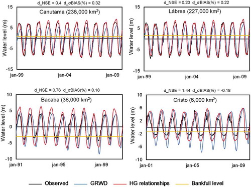
At the Lábrea and Canutama stations (stations located on the Purus River), there was an improvement in the simulation of the maximum and minimum water levels (anomalies), which demonstrates the efficiency of the HG relationships refinement in relation to the GRWD data for the purpose of representing the channel geometry of these gauge stations. This is because GRWD data overestimate the width and underestimate the depth of the channel cross-sections in relation to the HG relationships, also underestimating the cross-sectional area, which causes river overflow to the floodplain to occur in advance, causing attenuation of water level peaks.

At the Bacaba and Cristo stations, water level simulations using both geomorphological databases, GRWD and HG relationships, proved to be inefficient in representing the peaks of the water level graphs compared to the observed data. According to Paiva (2009), this is because in tributaries of large rivers, where water levels are controlled by the flooding of both rivers, errors in the estimation of bottom water levels by the MGB model can cause errors associated with the shape and to the time of the water level graphs over time in the affluent.

It can also be seen in Fig. 7 that for all gauge stations analysed, the floods are recurrent, regardless of the size of the drainage area; that is, the observed water levels of the river exceed the bankfull water level during a certain period of the year, usually between January and July. This explains why the use of HG relationships for the Purus River basin had a significant effect on the streamflow and water level modelling, since the MGB SA model is highly sensitive to changes in width and depth in cross sections that have extensive floodplains, such as those in the Amazon region.

4 Conclusions

Based on the objectives proposed in this study and the results obtained, the following can be concluded:

• The geographical convenience method allowed the definition of hydrologically homogeneous regions for the Purus River basins, as it was able to be sensitive to different relief patterns, precipitation regimes and flow regimes;

• The hydraulic geometry relationships for the entire basin obtained for the Purus River basin improved the width and depth estimates compared to data from the GRWD global database;

• The use of more refined Hydraulic Geometry relationships provided an improvement in the performance of the streamflow and water level modelling with the MGB SA model in the Purus River basin because the improvement of the representation of the channel geomorphology has greater effects in low slope rivers in regions with large floodplains, such as many sub-basins of the Amazon Basin;

• The use of more refined hydraulic geometry relationships for the Purus River basin provided an improvement in the modelling performance of the water level peaks in relation to the GRWD data, since these underestimate the area of channel cross-sections, causing attenuation of water level peaks;

• The Hydraulic Geometry relationships obtained in this study can be used to obtain more representative geomorphological input parameters to hydrological models, improving their predictive capabilities and having an impact on flood forecasting and water resource management in the Amazon region; and

• The methodology to develop more refined HG relationships can be applied to other river basins to obtain more reliable channel width and depth estimates where cross-section data are less available.

Acknowledgements

The authors would like to express their gratitude to Fundação de Amparo à Pesquisa do Estado de Minas Gerais (FAPEMIG), Coordenação de Aperfeiçoamento de Pessoal de Nível Superior (CAPES) and Conselho Nacional de Desenvolvimento Científico e Tecnológico (CNPq) for the financial support for the project under which this research was carried out.

Data availability statement

Some or all data, models, or codes that support the findings of this study are available from the corresponding authors upon reasonable request.

Disclosure statement

No potential conflict of interest was reported by the author(s).

Additional information

Funding

This work was supported by the Conselho Nacional de Desenvolvimento Científico e Tecnológico (CNPq) [165555/2017-3]; Fundação de Amparo à Pesquisa do Estado de Minas Gerais [545].

References

- Adeyemi, O., Olutoyin, F., and Olumide, O., 2020. Downstream hydraulic geometry across headwater channels in Upper Ogun River Basin, Southwestern Nigeria. African Geographical Review, 39 (4), 345–360. doi:10.1080/19376812.2020.1720756
- Alsdorf, D., et al., 2007. Spatial and temporal complexity of the Amazon flood measured from space. Geophysical Research Letters, 34 (8). doi:10.1029/2007GL029447
- Andreadis, K.M., Brinkerhoff, C.B., and Gleason, C.J., 2020. Constraining the assimilation of SWOT observations with hydraulic geometry relations. Water Resources Research, 49 (10), e2019WR026611.
- Andreadis, K.M., Schumann, G.J.P., and Pavelsky, T., 2013. A simple global river bankfull width and depth database. Water Resources Research, 49 (10), 7164–7168. doi:10.1002/wrcr.20440
- Bieger, K., et al., 2015. Development and evaluation of bankfull hydraulic geometry relationships for the physiographic regions of the United States. Journal of the American Water Resources Association, 51 (3), 842–858. doi:10.1111/jawr.12282
- Bravo, J.M., et al., 2012. Coupled hydrologic-hydraulic modeling of the Upper Paraguay River basin. Journal of Hydrologic Engineering, 17 (5), 635–646. doi:10.1061/(ASCE)HE.1943-5584.0000494
- Coe, M.T., Costa, M.H., and Howard, E.A., 2008. Simulating the surface waters of the Amazon River basin: impacts of new river geomorphic and flow parameterizations. Hydrological Processes: An International Journal, 22 (14), 2542–2553. doi:10.1002/hyp.6850
- Collischonn, W., 2001. Hydrological simulation of large basins (in Portuguese). Thesis (Doctorate in Water Resources and Environmental Sanitation). Porto Alegre, RS: Universidade do Rio Grande do Sul.
- Dalagnol, R., et al., 2017. Assessment of climate change impacts on water resources of the Purus Basin in the southwestern Amazon. Acta Amazonica, 47 (3), 213–226. doi:10.1590/1809-4392201601993
- Dunne, T. and Leopold, L.B., 1978. Water in environmental planning. San Francisco: W. H. Freeman.
- Durand, M., et al., 2016. An intercomparison of remote sensing river discharge estimation algorithms from measurements of river height, width, and slope. Water Resources Research, 52 (6), 4527–4549. doi:10.1002/2015WR018434
- Espinoza Villar, J.C., et al., 2009. Spatio‐temporal rainfall variability in the Amazon basin countries (Brazil, Peru, Bolivia, Colombia, and Ecuador). International Journal of Climatology: A Journal of the Royal Meteorological Society, 29 (11), 1574–1594.
- Fagundes, H.D.O., et al., 2017. Preliminary hydrosedimentological simulation in the Doce river Basin with the MGB SED model (in Portuguese). In: II Congresso Internacional de Hidrossedimentologia (2.: 2017: Foz do Iguaçu). Anais, 1–8. Foz do Iguaçu: Interciência.
- Fan, F.M., et al., 2016. Flood forecasting on the Tocantins River using ensemble rainfall forecasts and real‐time satellite rainfall estimates. Journal of Flood Risk Management, 9 (3), 278–288. doi:10.1111/jfr3.12177
- Filizola, N., et al., 2011. The flow of suspended matter in the Western Amazon as a marker of fluvial dynamics (in Portuguese). Manaus, Ed. Purus River: waters, territory and society in the South-Western Amazon (in Portuguese). Chapter 6.
- Fleischmann, A., Paiva, R., and Collischonn, W., 2019. Can regional to continental river hydrodynamic models be locally relevant? A cross-scale comparison. Journal of Hydrology X, 3, 100027. doi:10.1016/j.hydroa.2019.100027
- Frasson, R. P. D. M., Pavelsky, T. M., Fonstad, M. A., Durand, M. T., Allen, G. H., Schumann, G., Lion, C., Beighley, R. E., and Yang, X., 2019. Global relationships between river width, slope, catchment area, meander wavelength, sinuosity, and discharge. Geophysical Research Letters, 46(6), 3252–3262. doi:10.1029/2019GL082027
- Getirana, A.C., 2010. Integrating spatial altimetry data into the automatic calibration of hydrological models. Journal of Hydrology, 387 (3–4), 244–255. doi:10.1016/j.jhydrol.2010.04.013
- Grimaldi, S., et al., 2018. Effective representation of river geometry in hydraulic flood forecast models. Water Resources Research, 54 (2), 1031–1057. doi:10.1002/2017WR021765
- Knoben, W.J., Freer, J.E., and Woods, R.A., 2019. Inherent benchmark or not? Comparing Nash–Sutcliffe and Kling–Gupta efficiency scores. Hydrology and Earth System Sciences, 23 (10), 4323–4331. doi:10.5194/hess-23-4323-2019
- Knoben, W.J., Woods, R.A., and Freer, J.E., 2018. A quantitative hydrological climate classification evaluated with independent streamflow data. Water Resources Research, 54 (7), 5088–5109. doi:10.1029/2018WR022913
- Latuf, M. and Amaral, E., 2016. Assessment of suspended sediment discharge in the Purus River basin, Brazil. International Journal of River Basin Management, 14 (4), 413–429. doi:10.1080/15715124.2016.1215322
- Leopold, L.B. and Maddock, T., 1953. The hydraulic geometry of stream channels and some physiographic implications. Vol. 252. Washington, DC: US Government Printing Office.
- Luo, X., et al., 2017. Modeling surface water dynamics in the Amazon Basin using MOSART-Inundation v1. 0: impacts of geomorphological parameters and river flow representation. Geosciences Model Development, 10 (3), 1233–1259. doi:10.5194/gmd-10-1233-2017
- Maechler, M., et al., 2019. Finding groups in data: cluster analysis extended. Rousseeuw et. R Packag. version 2.0, 6.
- Meade, R.H., et al., 1991. Backwater effects in the Amazon River basin of Brazil. Environmental Geology and Water Sciences, 18 (2), 105–114. doi:10.1007/BF01704664
- Morel, M., et al., 2020. Intercontinental predictions of river hydraulic geometry from catchment physical characteristics. Journal of Hydrology, 582, 124292. doi:10.1016/j.jhydrol.2019.124292
- Moriasi, D.N., et al., 2015. Hydrologic and water quality models: performance measures and evaluation criteria. Transactions of the ASABE, 58 (6), 1763–1785.
- Muste, M., Ho, H.C., and Kim, D., 2011. Considerations on direct stream flow measurements using video imagery: outlook and research needs. Journal of Hydro-environment Research, 5 (4), 289–300. doi:10.1016/j.jher.2010.11.002
- Naghettini, M. and Pinto, É.J.D.A., 2007. Statistical hydrology (in Portuguese). Brazil: CPRM.
- Paiva, R.C., Collischonn, W., and Tucci, C.E., 2011. Large scale hydrologic and hydrodynamic modeling using limited data and a GIS based approach. Journal of Hydrology, 406 (3–4), 170–181. doi:10.1016/j.jhydrol.2011.06.007
- Paiva, R.C.D., et al., 2013. Large‐scale hydrologic and hydrodynamic modeling of the Amazon River basin. Water Resources Research, 49 (3), 1226–1243. doi:10.1002/wrcr.20067
- Paiva, R.D., 2009. Hydrological and hydrodynamic modeling of large basins. Study case: Solimões river basin (in Portuguese). MSc dissertation. Porto Alegre, Brazil: Instituto de Pesquisas Hidráulicas, Universidade Federal do Rio Grande do Sul, 182.
- Paiva, R.D., 2012. Hydrologie du bassin amazonien: compréhension et prévision fondées sur la modélisation hydrologique-hydrodynamique et la télédétection. Doctoral dissertation. Brasil: Université de Toulouse, Université Toulouse III-Paul Sabatier; Universidade Federal do Rio Grande do Sul.
- Peel, M.C., Finlayson, B.L., and McMahon, T.A., 2007. Updated world map of the Köppen-Geiger climate classification. Hydrology and Earth System Sciences Discussions, 4 (2), 439–473.
- Pontes, P.R.M., et al., 2017. MGB IPH model for hydrological and hydraulic simulation of large floodplain river systems coupled with open source GIS. Environmental Modelling Software, 94, 1–20. doi:10.1016/j.envsoft.2017.03.029
- R Core Team, 2014. R: a language and environment for statistical computing. Vienna, Austria: R Foundation for Statistical Computing.
- Rennó, C.D., et al., 2008. HAND, a new terrain descriptor using SRTM-DEM: mapping terra-firme rainforest environments in Amazonia. Remote Sensing of Environment, 112 (9), 3469–3481. doi:10.1016/j.rse.2008.03.018
- Ríos-Villamizar, E.A., et al., 2017. Surface water quality and deforestation of the Purus river basin, Brazilian Amazon. International Aquatic Research, 9 (1), 81–88. doi:10.1007/s40071-016-0150-1
- Siqueira, V.A., et al., 2016. Ensemble flood forecasting based on operational forecasts of the regional Eta EPS in the Taquari-Antas basin. Revista Brasileira de Recursos Hídricos, 21 (3), 587–602. doi:10.1590/2318-0331.011616004
- Siqueira, V.A., et al., 2018. Toward continental hydrologic–hydrodynamic modeling in South America. Hydrology and Earth System Sciences, 22 (9), 4815–4842. doi:10.5194/hess-22-4815-2018
- Sousa, H.T., et al., 2009. SISCAH 1.0: computational system for hydrological analysis (in Portuguese). Brasília, DF: ANA. Viçosa, MG: UFV.
- Sutanudjaja, E.H., et al., 2018. PCR-GLOBWB 2: a 5 arcmin global hydrological and water resources model. Geoscientific Model Development, 11 (6), 2429–2453. doi:10.5194/gmd-11-2429-2018
- Yamazaki, D., et al., 2011. A physically based description of floodplain inundation dynamics in a global river routing model. Water Resources Research, 47 (4), 4. doi:10.1029/2010WR009726