Water yield variability and response to climate change across Canada

ABSTRACT

This study generated a water yield dataset for Canada for 1979–2016 by subtracting the land surface evapotranspiration (ET) and water surface evaporation (E0) from precipitation (P). The dataset was validated in Budyko space and compared with streamflow (Q) before the spatial variability and trends were analysed. Results indicate (1) uncertainties of the dataset are generally small; (2) despite the asynchronous inter-annual change, annual water yield varies in a similar temporal pattern to Q; (3) annual water yield varies dramatically across Canada, ranging from about zero on the Canadian Prairies to over 2500 mm on the West Coast; and (4) annual water yield shows no significant changes over the study period in the vast majority (82.4%) of Canada’s landmass. The most significant increasing trend appears in South Central Canada, attributed to increasing P. The most significant decreasing trend appears in Northeast Canada and the Southern Montane Cordillera, attributed to decreasing P and increasing ET.

KEYWORDS:

• water yield
• Canada landmass
• climate change
• streamflow
• Budyko space

Editor A. Fiori Associate Editor R. Singh

1 Introduction

How regional water availability responds to climate change is one of the most critical issues to be addressed for sustainable water resource management (Jackson et al. 2001, Gordon and Famiglietti 2004, Piao et al. 2010). Regional water availability can be measured by water yield, defined as precipitation (P) minus evapotranspiration (ET). Calculating water yield has been challenging because of the difficulties quantifying regional ET and P, which are both highly spatially and temporally variable. Recent advances have been made in quantifying long-term ET from land surface models and remote sensing approaches at local, regional, and global scales (Oleson et al. 2008, Wang et al. 2013, Fisher et al. 2017) and in improving the quality of gridded P data (Sheffield et al. 2006). Such advancements have made it possible to generate spatially and temporally continuous water yield datasets. However, no such water yield data is available yet in Canada.

Water yield and its response to climate change are expected to be highly variable in space and time (Davi et al. 2006, Vicuna and Dracup 2007, Barontini et al. 2009, Gautam and Acharya 2012). Water yield is a function of various factors, including climate and land surface characteristics (Sun et al. 2006). The varying climatic variables and land surface characteristics and their interactions lead to a highly variable water yield response to climate change. Investigating the spatial variability and the long-term trends of water yield at multiple temporal scales is critical for understanding the hydrological response to climate change and, further, for sustainable water resource management (Burkhard et al. 2012, Yu et al. 2015, Wang et al. 2020).

Globally, contrasting trends of water yield during different periods were found in response to climate change. A decreasing trend of water yield has been reported in many studies (Zhang et al. 2001, Déry and Wood 2005, Wang et al. 2008, López-Moreno et al. 2011), while an increasing trend has also been detected (Lins and Slack 1999, Peng and Xu 2010). The changes were attributed to different driving factors (Stahl et al. 2010, Gudmundsson et al. 2019). Some studies found that the changes in water yield are accounted for by the variations in ET (López-Moreno et al. 2011), but others stated that P is the most influencing variable on water yield (Déry and Wood 2005, Wang et al. 2008, Lu et al. 2013). The inconsistent trends and influencing factors may result from the differences in study period and scale, analytical methods, and climate conditions, and the magnitude of climate change (Lu et al. 2013). Applying a uniform approach to spatially and temporally continuous datasets to investigate the evolution of water yield across diverse environments can help us better understand climate change impacts on the hydrological cycle.

In this study, we generated a water yield dataset for Canada’s entire landmass in 1979–2016 by subtracting ET (Wang et al. 2013) and water surface evaporation (E0) (Li et al. 2020) simulated in the Ecological Assimilation of Land and Climate Observations (EALCO) model from the global precipitation data produced by Princeton University (Sheffield et al. 2006). The datasets were generated at a daily temporal scale and aggregated into monthly and annual scales. The dataset was compared with streamflow (Q) measurements and validated in the Budyko space before analysing the spatiotemporal variability and trends. Our objectives were to characterize the spatiotemporal variability of water yield and analyse the long-term trends and climate drivers of water yield change at multiple time scales. Canada encompasses a diverse climate that varies dramatically, from cold and dry Arctic to semiarid Prairies to mountain climate to humid maritime climate. By applying consistent data and methods to analyse the spatial variability and long-term trends of water yield for this landmass, this study provides insight into hydrological response to climate change.

2 Materials and methods

2.1 Water yield dataset generation

Water yield (WY) over a given time period (e.g. daily, monthly, and annual) can be calculated using Equation (1)(1) $WY=P-\left(1.0-\alpha \right)ET-\alpha E0$(1) :

(1) $WY=P-\left(1.0-\alpha \right)ET-\alpha E0$(1)

where $P$ is precipitation, $ET$ is land surface evapotranspiration, E0 is water surface evaporation, and $\alpha$ is a parameter representing the water surface fraction in a pixel (10 km × 10 km in this study), calculated by Wang et al. (2014a).

2.1.1 Land surface evapotranspiration (ET) and water surface evaporation (E0)

ET and E0 data were generated using the land surface model EALCO, developed for simulating terrestrial ecosystem-atmosphere interactions using in situ and remote sensing observations (Wang et al. 2013). The model simulates the dynamic land surface processes of radiation transfer (Wang 2005, Wang et al. 2007), water transfer (Wang 2008, 2012), energy balance (Wang et al. 2002a, 2009, Zhang et al. 2008), and carbon and nitrogen biogeochemical cycles (Wang et al. 2001, 2002b), and their physical and physiological controls in ET. Developed in Canada, the model has particularly comprehensive algorithms for simulating the land surface processes in cold regions.

ET and E0 were simulated in the EALCO model driven by the atmospheric forcing of Sheffield et al. (2006) and parameterized by the remotely sensed land surface vegetation data and inventory soil maps (Wang et al. 2013). ET includes canopy transpiration through leaf stomata, canopy evaporation of intercepted rain or dew, canopy sublimation of intercepted snow or frost, soil evaporation and snow sublimation at the ground surface, and evaporation of water from temporary puddles after rain events (Wang et al. 2013). The simulated ET is at a 5-km spatial resolution and a 30-min time step. EALCO E0 was calculated at a daily time step, and it was mainly based on the Penman equation and the dynamic seasonal surface evolutions of water-ice-snow (Li et al. 2020). Evaluations of EALCO ET for Canada’s landmass have been conducted using ET from other land surface models, the Moderate Resolution Imaging Spectroradiometer (MODIS) ET products from remote sensing, water budget approach, and in situ tower flux measurements (Wang et al. 2015a). The EALCO model ET has also been tested in diverse ecosystems in several modelling studies, including the Boreal Ecosystem-Atmosphere Study (BOREAS) (Amthor et al. 2001, Potter et al. 2001), the AmeriFlux Network (Hanson et al. 2004), the Fluxnet Canada Research Network (FCRN) (Grant et al. 2005, 2006, 2009), and the Free-Air CO₂ Enrichment (FACE) Model-Data Synthesis study (Walker et al. 2014, Medlyn et al. 2015). The regional composite of ET and E0 based on the water surface fraction for a region has been assessed by examining water budget closures for all gauged watersheds in Canada (Wang et al. 2014a, 2014b, 2015a).

2.1.2 Precipitation (P)

The precipitation dataset was produced by the Terrestrial Hydrology Research Group at Princeton University by fusing a suite of global observation-based datasets into the National Centers for Environmental Prediction (NCEP)/National Center for Atmospheric Research (NCAR) data. Details on the dataset were introduced in Sheffield et al. (2006), with later updates in (https://hydrology.princeton.edu/data.pgf.php). The datasets are available at a 0.25-degree spatial resolution and a 3-h time scale and were downscaled to 10 × 10 km² grids using bilinear interpolation for this study (Wang et al. 2013).

2.2 Water yield data validation

For a given period, the water budget in a drainage basin can be described as:

(2) $WY=Q+\mathrm{\Delta }TWS$(2)

where Q is streamflow, and $\mathrm{\Delta }TWS$ is total water storage change, including surface waters, soil moisture, glaciers, groundwater, snowpack, and canopy water.

In a short period (e.g. annual or monthly), $\mathrm{\Delta }TWS$ can play a significant role and consequently leads to the difference in the values of Q and water yield. In the long term (38 years in this study), $\mathrm{\Delta }TWS$ is often negligible, and water yield equals Q. In this study, annual and monthly water yield were compared with Q in the 19 drainage basins (Fig. 1, Section 2.2.1). The long-term mean of the water yield dataset was validated in the Budyko space in the basins (Section 2.2.2).

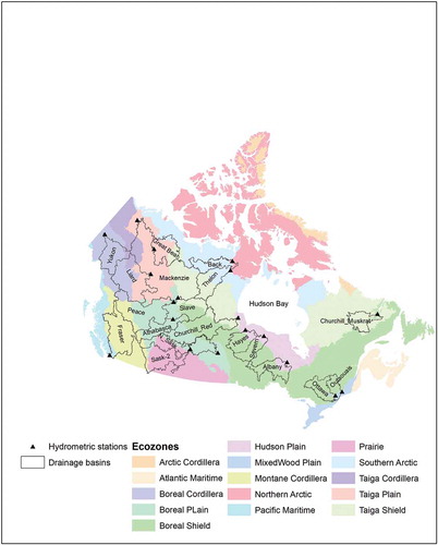
Figure 1. Spatial distribution of the 19 large drainage basins, hydrometric stations, and 15 ecozones in Canada

2.2.1 Comparision between water yield and streamflow (Q)

Water yield and Q were compared at annual and monthly scales in the 19 drainage basins (Fig. 1, Table 1). The monthly Q data (m³ s⁻¹) in the drainage basins were obtained from the Water Survey of Canada website (https://www.canada.ca/en/environment-climate-change/services/water-overview/quantity/monitoring/survey/data-products-services/national-archive-hydat.html). The Q values were divided by the drainage areas to obtain the water depth (mm) in each watershed. The Q data record in the 19 watersheds ranges from 13 to 38 years (Table 1). The water surface fraction ranges from 0.01 in the Liard basin to 0.31 in the Great Bear Lake basin (Wang et al. 2014b).

Table 1. The drainage basins, hydrometric station number (STNNBR), gross drainage area (Area, 103 km²), the number of years having streamflow (Q) observations (NY), mean annual Q (mm), evapotranspiration (ET, mm), water surface evaporation (E0, mm), precipitation (P, mm), and water yield (WY, mm) in 1979–2016 (Sask-2* is the portion of the Saskatchewan River at Grand Rapids drainage basin after the North Saskatchewan basin is separated out)

Basins	STNNBR	Area	NY	Q	ET	E0	P	WY
Mackenzie	10LC014	651.7	36	127	244.4	538.1	322.7	78.3
Liard	10ED002	275	38	287.4	274.9	581.9	465.5	190.6
Thelon	06MA006	152	29	194.0	211.7	432.7	295.8	84
Back	10RC001	93.9	29	165.8	185.3	389.7	239.3	54.1
Great Bear	10JC003	146.4	16	118.3	256.8	477.6	256.6	−0.2
Yukon	09CD001	149	38	258.2	199.0	517.2	289.0	90
Fraser	08MH024	228	14	442.7	398.8	667.3	734.8	336
N_Sask	05GG001	131	38	56.4	408.5	742.4	493.4	85
Hayes	04AB001	103	13	197.9	329.1	639.6	541.6	212.5
Sask-2*	05KL001	275	36	39.3	395.2	810.8	439.4	44.2
Athabasca	07DA001	133	38	137.5	393.8	702.8	525.7	131.9
Slave	07NB001	180	34	109.5	267.0	614.2	408.7	141.7
Peace	07KC001	293	32	219.1	372.0	664.0	502.2	130.2
Churchill_Red	06FD001	289	20	33.0	341.6	659.5	471.2	129.6
Ottawa	02KF005	90.9	37	427.1	563.5	809.5	939.3	375.8
Severn	04CC001	94.3	13	194.3	355.4	656.6	603.7	248.3
Albany	04HA001	118	30	269.0	423.9	721.1	725.5	301.6
Churchill_Muskrat	03OE001	92.5	36	615.6	292.0	556.5	876.1	584.1
Outaouais	02LB024	143	16	430.7	507.9	773.1	1010.8	502.9

2.2.2 Long-term mean water yield validation in the Budyko space

Provided $\mathrm{\Delta }TWS$ is negligible in the long term in a basin, the scatter point(s) of the calculated evaporative index (EI = ET/P) and aridity index (AI = E0/P) should fall precisely onto the Budyko curve that describes the partitioning of P between Q and ET (Budyko 1963, Fang et al. 2016). This allows the validation of the long-term means of P and ET in the Budyko space, assuming that their errors are analogous to ET/P and E0/P. The uncertainties in P and ET, therefore, can be estimated by calculating the smallest Euclidean distance between the (AI, EI) and the basin-specific Budyko curve (Greve et al. 2014, Koppa and Gebremichael 2017).

(3) $O{D}_{min}=\sqrt{{(A{I}_{est}-AI)}^2+{(E{I}_{est}-E{I}_{mod})}^2}$(3)

where $O{D}_{min}$, the minimum Euclidean distance, represents the combined errors of the P and ET datasets in representing the long-term water and energy balance. A smaller $O{D}_{min}$ means less uncertainty in the combined datasets. $A{I}_{est}$ and $E{I}_{est}$ are the long-term average of AI and EI, respectively, calculated from the EALCO ET, E0, and Princeton P data. EI_mod is the EI calculated using Fu’s equation (Fu 1981):

(4) $E{I}_{mod}=1+AI-{\left(1+A{I}^w\right)}^{1/w}$(4)

where $w$ is a parameter representing the impacts of underlying basin characteristics, including vegetation coverage, geomorphic feature, soil properties in the watershed, and climate seasonality, on the Budyko curve (Xu et al. 2013).

The estimation of $w$ is scale dependent. Li et al. (2013) and Xu et al. (2013) developed equations to estimate $w$ for basins with different areas. In this study, four of the 19 basins have an area > 230 000 km², and no basins have areas < 10 000 km² (Table 1). We thus estimated $w$ using the equations developed for the basins having areas > 230 000 km² and < 10 000 km² (Equation(5)(5) $w=3.50412-0.09311slp-0.03288lat+1.12312NDVI-0.00205lon-0.00026elev$(5) ), and the basins > 230 000 km² (see Supplementary material, Equation (S2)) (Xu et al. 2013). We also used the equation of Li et al. (2013) (see Supplementary material, Equation (S3)) because of its simplicity, with the normalized difference vegetation index (NDVI) as the only independent variable.

(5) $w=3.50412-0.09311slp-0.03288lat+1.12312NDVI-0.00205lon-0.00026elev$(5)

where lat and lon are the latitude and longitude of the basin centre, respectively; slp is the slope of the terrain; elev is the averaged elevation; and NDVI is the mean annual normalized difference vegetation index in 1981–2016. Slope and elevation were extracted from the United States Geological Survey (USGS) Global 30 Arc-Second Elevation (GOTOP30) data (https://earthexplorer.usgs.gov/). The NDVI used is the Global Inventory Modeling and Mapping Studies (GIMMS) 8-km bi-monthly the Advanced Very-High-Resolution Radiometer (AVHRR) NDVI dataset (1981–2006) (Tucker et al. 2004, 2005) (http://iridl.ldeo.columbia.edu/SOURCES/.UMD/.GLCF/.GIMMS/.NDVIg/.global/.ndvi/dods) and 1-km MODIS 16-d NDVI datasets (2007–2016) from Google Earth Engine. The AVHRR and MODIS NDVI are generally consistent (Brown et al. 2006), and therefore the influence of using two NDVI datasets on $w$ is expected to be nonsignificant. The NDVI, slp, and elev used are the spatial mean in each basin.

2.3 Spatial variability, seasonal variations, and long-term trends of water yield

The spatial variability of long-term means and trends of annual and monthly water yield in 1979–2016 were analysed across Canada. Monthly water yield was summed to obtain the total water yield in the cold season (October–April) because of its potential effects on early spring floods. The total water yield in the warm season (May–September) was also investigated because the peak of water use typically occurs in that period. Finally, annual and monthly water yield were aggregated at the ecozone scale (Fig. 1) for ecohydrologists with an interest in studying the ecosystem functions and services.

The water yield trends at multiple temporal scales (i.e. annual, monthly, and seasonal) were analysed using the non-parametric Mann-Kendell (M-K) test (Mann 1945, Kendall 1975). Sen’s slope was used to indicate the trends, and the 95% confidence interval (p < 0.05) was applied to identify the statistically significant changes. The trends of P and ET at the corresponding time scales were also investigated to determine the driving factors of water yield change. No autocorrelation was detected in the annual water yield time series (see Supplementary material, Fig. S1). Hence, the M-K test was directly applied to the original datasets.

3 Results

3.1 Water yield validation

3.1.1 Comparisons between water yield and Q

Annual water yield generally has a similar inter-annual variation pattern to Q in all basins; however, the two variables change asynchronously in some years (Fig. 2). P from snowfall in the cold season accumulates and forms snowpacks, eventually contributing to Q in the following year. This phenomenon is unique to cold regions.

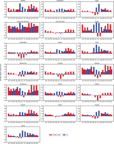
Figure 2. Temporal variations of annual water yield and streamflow (Q) in the 19 basins of Canada, 1979–2016 (Q data availability varies among basins, as presented in Table 1)

The difference in the values of annual water yield and Q varies among basins. Water yield is generally close to Q in the Ottawa, Albany, and Churchill-Muskrat basins in Eastern Canada, although a relatively larger discrepancy is observed in some years. Water yield is mostly greater than Q in the N-Sask and Sask-2 basins in Canadian Prairies, possibly due to agriculture/industry (e.g. resources development) water use. Water yield is less than Q in the Mackenzie, Yukon, Liard, and Thelon basins in Northwest Canada, possibly because of the influence of glacier/permanent snowmelt from the Rocky Mountains on the headwater Q and/or the increased groundwater discharge as a result of permafrost degradation (Walvoord and Striegl 2007, Wang 2019).

The seasonal variation of monthly water yield is opposite to that of Q (Fig. 3). Water yield shows a distinct seasonal variation, with higher values in the cold season but lower numbers in the warm season. Water yield in the cold season is mainly controlled by P, because ET is low in the vast area of Canada. From the cold to the warm season, water yield decreases as ET increases. Negative water yield in the warm season appears in 14 of 19 basins because ET is higher than P. In contrast, Q typically is lower in the cold season than in the warm season, except for the Great Bear Lake basin, where the seasonal variation of Q is small. The lower Q in the cold season is accounted for by the limited surface runoff from rain and low baseflow from groundwater discharge due to frozen soils (Wang 2019), while the higher Q in the warm season results from snowmelt runoff in spring and high precipitation in summer.

Figure 3. The seasonal variations of monthly water yield and streamflow (Q) in the 19 basins of Canada, 1979–2016 (the periods for comparison between water yield and Q vary among basins, depending on the number of years of Q observations, as listed in Table 1)

Besides the comparisons with Q, the P and ET data used in this study were also compared with the other independent P and ET data. The P data was compared with a different dataset generated by interpolating observations at climate stations. The comparison shows that the difference between the two P datasets varies from −15% to +22% in 16 of the 19 basins investigated. ET was compared with the other datasets simulated using the Community Land Model (CLM) and Variable Infiltration Capacity (VIC) models over Canada, showing small differences (Wang et al. 2015b).

3.1.2 P and ET datasets in the Budyko space

The long-term means of P and ET were validated in the Budyko space. The closer to the Budyko curve, the smaller the distance $(O{D}_{min})$ and the less uncertainty in the P and ET datasets. The validation against the Budyko parameter estimated using Equation (5)(5) $w=3.50412-0.09311slp-0.03288lat+1.12312NDVI-0.00205lon-0.00026elev$(5) is shown in Fig. 4. The other validation, using the parameter calculated using Equations (S2) and (S3), is presented in the Supplementary material.

Figure 4. The long-term mean evaporative index (EI), aridity index (AI) and Budyko curve in the 19 large basins in Canada. (The Budyko parameter, $w$, was estimated using Xu et al. (2013)’s equation developed for combined basins having an area smaller than 10 000 km² and larger than 230 000 km². It is shown as the number in parentheses following the name of the drainage basin)

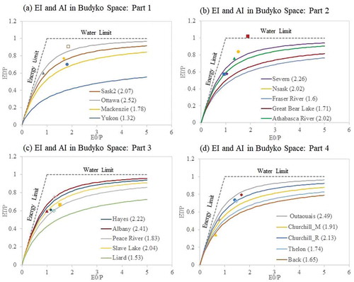
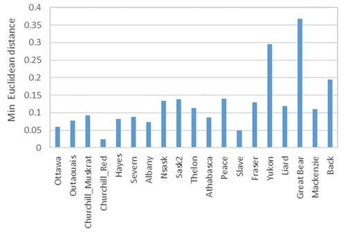
The parameter $w$ estimated for the same basin varies using the three equations, resulting in different distances between the (AI, EI) point and the Budyko curve (see Fig. 4 and Supplementary material, Figs S2 and S4). For example, in the North Saskatchewan River (N_Sask) and South Saskatchewan River (Sask-2), the distance $(O{D}_{min})$ is > 0.10 when $w$ was calculated using Equations (5)(5) $w=3.50412-0.09311slp-0.03288lat+1.12312NDVI-0.00205lon-0.00026elev$(5) and (S3) (see Fig. 4 and Supplementary material, Fig. S4), but the distance is <0.05 when $w$ was estimated using Equation (S2) (see Supplementary material, Fig. S2). However, generally, the distance is < 0.15 in most basins (see Fig. 5 and Supplementary material, Figs S3 and S5).

Figure 5. The uncertainties in water yield measured by the minimum Euclidean distance ($O{D}_{min})$ between the long-term mean evaporative index (EI) and aridity index (AI) and the Budyko curve in the 19 large basins in Canada. (The Budyko parameter, $w$, was estimated using Xu et al. (2013)’s equation developed for combined basins having an area smaller than 10 000 km² and larger than 230 000 km²)

Ideally, the long-term EI and AI scattered points should fall exactly onto the curve; however, all data have uncertainties. The P-ET is likely the most uncertain component in the water budget (Barontini et al. 2009). The off-curve points indicate the imbalance between water yield and Q, implying the unclosed water budget in Canada, as reported by Wang et al. (2014a, 2014b, 2015a). Besides, the estimated $w$ for the Budyko curve may also contain uncertainties propagated from the Digital Elevation Model (DEM) and NDVI data and the empirical equations, accounting for the imbalance.

3.2 Water yield variability

3.2.1 Annual water yield

Figure 6 shows the long-term means of annual water yield in 1979–2016. Annual water yield demonstrates large spatial variability. High water yield (> 800 mm) occurs on the West Coast, in theSouthern Montane Cordillera, and in Eastern Canada. The maximum water yield on the West Coast can reach over 2500 mm. Annual water yield in other areas is generally lower than 300 mm, with values close to zero in some regions of the Canadian Prairies and Northern Canada. Negative water yield occurs in large water bodies where water surface evaporation exceeds precipitation.

Figure 6. The spatial variations of annual water yield (mm) averaged over Canada’s landmass, 1979–2016

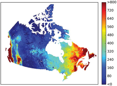
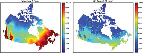
The spatial distribution of annual water yield is generally consistent with annual P, with high values on the West Coast, in the Southern Montane Cordillera, and in Eastern Canada (Figs 6 and 7(a)). However, ET’s role is also evident in some regions, such as Southeast Canada, where high ET offsets the relatively high P, resulting in less water yield than in Northeast Canada (Figs 6, 7(a) and (b)).

Figure 7. The spatial variations of (a) annual precipitation (P, mm) and (b) annual evapotranspiration (ET, mm) demonstrated by their long-term means over Canada’s landmass, 1979–2016

3.2.2 Seasonal variations of water yield

Monthly water yield has higher values in the cold season than in the warm season (Fig. 8), as shown at the basin scale (Fig. 3). In the cold season, monthly water yield varies across space, with the high values (200–480 mm) on the West and East coasts. The total water yield in the cold season varies from several tens of mm in the Northwest to approximately 1800 mm on the West Coast (see Supplementary material, Fig. S6a). The spatial distribution of monthly water yield and the total water yield in the cold season are mainly controlled by P (see Fig. 9 and Supplementary material, Fig. S7). Monthly ET is generally less than 30 mm (Fig. 10) and has little influence on the spatial distribution of water yield.

Figure 8. Mean monthly water yield (mm) across Canada, 1979–2016

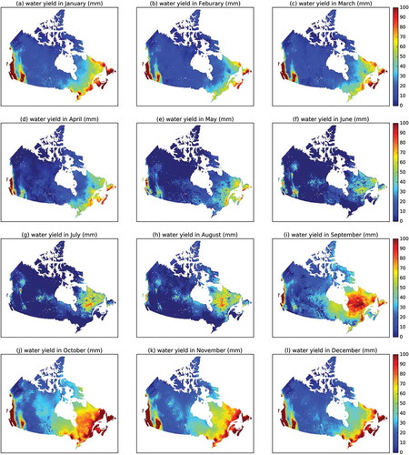
Figure 9. Mean monthly precipitation (P, mm) across Canada, 1979–2016

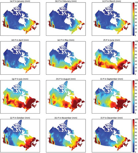
Figure 10. Mean monthly evapotranspiration (ET, mm) across Canada, 1979–2016

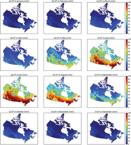
In the warm season, monthly water yield is mainly maximized in Northeast Canada (approximately 100 to > 200 mm). The West Coast and Southern Montane Cordillera also have high water yield in May, June, and September. Monthly water yield in the other regions is generally less than 30 mm (Fig. 8). The total water yield in the warm season is high as 200 to over 500 mm on the West Coast and in Northeast Canada, and is less than 200 mm or even close to zero in the other regions (see Supplementary material, Fig. S6b). The spatial distribution of monthly water yield in the warm season is influenced by P and ET (see Supplementary material, Figs S6 and S7). For example, the high P in southern Canada is offset by the high ET, resulting in the relatively low monthly water yield in May to August (Figs 8–10).

When aggregated at the ecozone scale (Table 2), monthly water yield has positive values in September to April in all of the ecozones, ranging from <10 mm in Janurary–April in the Northern Arctic to 257 mm in November in the Pacific Maritime Ecozone. Monthly water yield in May to August is generally < 50 mm, with some negative values observed because ET is greater than P. Annually, water yield varies from 15 mm in the Prairies to 1494 mm in the Pacific Maritime Ecozone, followed by 719 mm in the Atlantic Maritime Ecozone. Water yield is between 300 mm and 500 mm in the Hudson Bay, Taiga Shield, Montane Cordillera, MixedWood Plain, and Boreal Shield ecozones. Water yield in the Arctic Cordillera and Boreal Cordillera is slightly lower than 200 mm, while in other regions it is under 100 mm.

Table 2. Monthly and annual water yield (WY, mm) aggregated in the ecozones

Ecozone	Monthly WY
	January	February	March	April	May	June	July	August	September	October	November	December	Annual WY
Arctic Cordillera	17	14	17	13	2	−4	−1	19	34	33	30	21	195
Northern Arctic	7	5	6	5	−4	−25	−15	9	22	24	16	10	62
Southern Arctic	11	9	10	5	−7	−22	−16	5	23	30	23	17	88
Taiga Plain	13	11	10	2	−10	−20	−18	0	10	23	18	16	56
Taiga Shield	29	20	25	16	9	9	17	30	51	53	45	34	337
Boreal Shield	58	40	44	35	29	16	7	17	52	76	69	65	506
Atlantic Maritime	97	69	87	71	54	3	−22	−8	46	103	106	114	719
MixedWood Plain	77	54	57	51	27	−32	−48	−3	57	78	82	90	489
Boreal Plain	18	12	14	3	−9	−18	−27	−16	11	20	21	19	49
Prairie	18	11	11	6	1	−27	−54	−20	17	17	17	19	15
Taiga Cordillera	10	10	10	0	−5	1	6	11	10	11	13	8	83
Boreal Cordillera	25	16	14	1	4	3	10	10	21	25	25	23	179
Pacific Maritime	229	143	154	97	48	23	−11	10	85	221	257	237	1494
Montane Cordillera	62	43	46	21	15	12	−18	−18	17	50	70	64	363
Hudson Plain	23	17	18	16	13	11	14	17	55	52	39	29	304

3.3 Water yield trends

3.3.1 Annual water yield

The long-term trends of annual water yield in Canada in 1979–2016 are shown in Fig. 11. Annual water yield shows significantly increasing trends at rates of 1.5–13 mm/year in South Central Canada and in small areas in the Northeast and West to Hudson Bay (Fig. 11). Significantly decreasing water yield trends are observed in Northeast Canada, Southern Montane Cordillera, and Northern Canada, and on the West Coast, at rates of −20 to −1 mm/year.

Figure 11. The trends of annual water yield (mm/year) by Sen’s slope over Canada’s landmass, 1979–2016 (hatching suggests that the trends are significant at the 95% confidence interval)

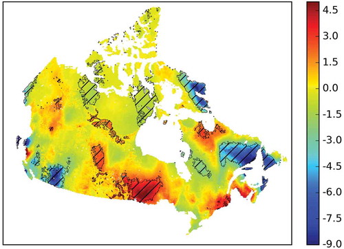
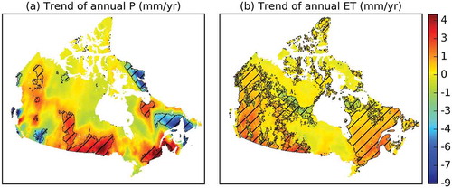
The spatial distribution of annual water yield trends is similar to that of annual P (Figs 11 and 12(a)), implying a dominant role for P in water yield change in Canada. ET has significantly increasing trends in Eastern and Western Canada (Fig. 12(b)), including on the West Coast and East Coast (Fernandes et al. 2007). The increasing ET intensified the decreasing water yield in Northeast Canada, Southern Montane Cordillera, and Northern Canada.

Figure 12. The trends of (a) annual precipitation (P, mm/year) and (b) annual evapotranspiration (ET, mm/year) by Sen’s slope over Canada’s landmass, 1979–2016 (hatching suggests that the trends are significant at the 95% confidence interval)

3.3.2 Monthly water yield

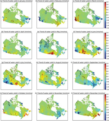
The long-term trend of monthly water yield in 1979–2016 is demonstrated in Fig. 13. Monthly water yield shows a significant change in some regions. Specifically, monthly water yield decreased at −4 to −1 mm/month in January, March, June, and September in Northeast Canada, accounting for the significantly decreasing annual water yield in the region. The decreasing water yield in February, July, and December in the Southern Montane Cordillera is the primary contributor to the decreasing annual trend in the region. The decreasing water yield in September in Southeast Canada is compensated by the increasing water yield in December, resulting in a nonsignificant trend at the annual scale. The increase of monthly water yield in May, June, and July at approximately 1 to > 4 mm/month in South Central Canada, accounts for the increasing annual trend in the region. A positive slope of monthly water yield is observed from October to April in South Central Canada; however, the slope is generally not statistically significant, except in December (Fig. 13(a)–(d) and (j)–(l)).

Figure 13. The trends of monthly water yield (mm/month) by Sen’s slope over Canada’s landmass, 1979–2016 (hatching suggests that the trends are significant at the 95% confidence interval)

To further evaluate the contribution of monthly water yield changes to the annual water yield trends, we analysed the total water yield trends in the cold season and in the warm season (see Supplementary material, Fig. S8). The total water yield in each season shows a significantly increasing trend in South Central Canada (see Supplementary material, Fig. S8a), implying their contribution to annual water yield increases in the region. The decreasing total water yield in the cold and warm seasons contributed to the annual water yield decrease in Northeast Canada and the Southern Montane Cordillera. However, annual water yield changes in some regions are caused only by the changes in the warm season or the cold season (not both). For example, the increasing annual water yield in the area northeast to Hudson Bay is caused by increased water yield in the warm season, and the decrease on the West Coast mainly results from the decreasd water yield in the cold season.

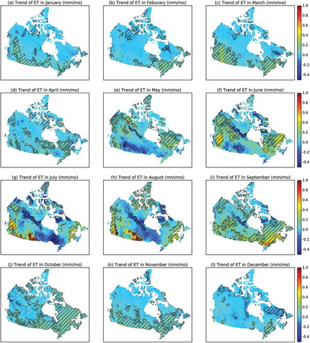
The significant water yield changes in the cold season are mainly accounted for by the changes of P (see Fig. 14 and Supplementary material, Fig. S9). In the warm season, the increasing water yield is attributed to the increasing P. However, ET plays a vital role in decreasing water yield, particularly in Western Canada in July and Eastern Canada in September (see Fig. 15 and Supplementary material, Fig. S9). Such roles of P and ET are also identified at the ecozone scale (see Supplementary material, Table S1).

Figure 14. The trends of monthly precipitation (P, mm/month) by Sen’s slope over Canada’s landmass, 1979–2016 (hatching suggests that the trends are significant at the 95% confidence interval)

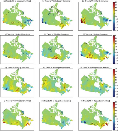
Figure 15. The trends of monthly evapotranspiration (ET, mm/month) by Sen’s slope over Canada’s landmass, 1979–2016 (hatching suggests that the trends are significant at the 95% confidence interval)

4 Discussion

4.1 Uncertainties in the water yield dataset

The water yield generated in this study quantifies the net water flux between the atmosphere and the land surface. In a drainage basin, water yield is typically assumed to be balanced with Q in the long term but different from Q in the short term due to the role of $\mathrm{\Delta }TWS$. It is challenging to directly validate the long-term means of water yield through a comparison with the measured Q in cold regions because of the relatively high uncertainties in P, Q, and ET (Yang et al. 2005, Shiklomanov et al. 2006, Wang et al. 2013). In this study, the long-term water yield was indirectly validated in the Budyko space based on P, ET, and E0, without introducing the uncertainties in Q. There is a short distance between the (ET/P, E0/P) and the Budyko curve in most basins, implying a small imbalance between long-term water yield and Q. The imbalance is consistent with the findings in various basins worldwide (Serreze et al. 2002, Marengo 2005, Wang et al. 2014a, 2014b). Furthermore, we should be aware that the Budyko parameter also has uncertainties propagated from the DEM and NDVI data errors.

4.2 The long-term trends of water yield and driving factors

Trends of water yield vary across space in Canada. The annual water yield trends are generally consistent with the streamflow trends published in the literature. For example, the decreasing water yield trends in Western Canada agree with the declining annual streamflow trends reported by Zhang et al. (2001). The decreasing water yield in Northeast Canada is consistent with the decreasing streamflow in rivers flowing to the Arctic oceans reported by Déry and Wood (2005). The nonsignificant water yield trend in the area northwest to Hudson Bay is consistent with the streamflow observations in the Kazan and Back rivers reported by Spence (2002). The increasing water yield trend in South Central Canada and on the East Coast is consistent with the annual streamflow trends reported by George (2007) and Nalley et al. (2012). It is worth noting that the increasing water yield in South Central Canada does not agree with the decreasing streamflow reported by Zhang et al. (2001), likely due to the difference in study periods.

Previous studies have found that monthly streamflow in the southern part of Canada decreased in most months, with the maximum decrease in August and September, but increased in March and April (Zhang et al. 2001). Burn and Elnur (2002) found increasing streamflow in March and April, and decreasing streamflow in June. This study found a significant water yield increase in March in Western Canada and April in the Southern Canadian Prairies (Fig. 10(c) and (d)). This study also found increasing total water yield in the cold season in South Central Canada and Southeast Canada (see Supplementary material, Fig. S6), consistent with the increasing streamflow in March and April attributed to the earlier snowmelt (Zhang et al. 2001, Burn and Elnur 2002). The negative slope of water yield in June to September agrees with decreasing streamflow; however, the significant water yield increase in South Central Canada in May to July was not consistent with decreasing streamflow (Zhang et al. 2001, Burn and Elnur 2002). This inconsistency is possibly caused by a difference in study periods. The changing water yield could substantially influence local water resources and add pressure to ecosystems (Mccabe and Wolock 1997), particularly in water-limited regions, such as the Canadian Prairies (Schindler and Donahue 2006).

This study identified increasing P as the primary driver for the regions with significantly ascending water yield, while decreasing P concurred with increasing ET to account for the regions with descending water yield trends. Previously, some studies reported that P has a primary influence on streamflow trends (Zhang et al. 2001, Déry and Wood 2005, George 2007), while other studies indicated that a change in ET dominates the water yield trends (Gedney et al. 2006, Betts et al. 2007). Recently, Padrón et al. (2020) stated that increasing ET intensified the dry-season water availability (the minimum monthly water yield), rather than decreasing precipitation, in Europe, western North America, southern South America, northern Asia, Australia, and Eastern Africa, from 1902 to 2014.

4.3 Contribution and future research

This study first generated a long-term spatially and temporally consistent water yield dataset, and analysed water yield variability and trends, for Canada’s entire landmass. The dataset was validated in the Budyko space based on the basin-specific Budyko parameter. The results contribute to understanding how water yield responds to climate change in diverse climate regions across Canada and have implications for sustainable freshwater and ecosystem management. Future studies should include the interactive effects of basin characteristics, local environment, and large-scale climate phenomena on water yield change at multiple temporal scales. Furthermore, the impact of anthropogenic activities, such as agriculture irrigation, water withdrawal for resources development, and land use and land cover change, on water yield should also be investigated in future studies.

5 Conclusions

This study generated a water yield dataset for all of Canada in 1979–2016 by subtracting the land surface evapotranspiration (ET) and water surface evaporation (E0) simulated by the Ecological Assimilation of Land and Climate Observations (EALCO) model from the global precipitation (P) data produced by Princeton University. The dataset was validated in the Budyko space and compared with streamflow (Q) in 19 basins before the spatial variability and trends at multiple temporal scales were analysed. The results show:

1. uncertainties in the long-term means of water yield are generally small, indicated by the minimum Euclidean distance between the (ET/P, E0/P) point and the basin-specific Budyko curve;

2. annual water yield varies in a similar temporal pattern to Q, altough the two variables change asynchronously in some years;

3. water yield varies dramatically across Canada, with high annual values of over 2500 mm on the West Coast and over 700 mm in Northeast Canada, and low values of close to zero on the Canadian Prairies;

4. water yield exhibits no significant changes in the vast majority (82.4%) of Canada’s landmass. For the rest of the landmass, annual water yield shows the most significantly increasing trends in South Central Canada, and decreasing trends in Northeast Canada and the Southern Montane Cordillera;

5. monthly water yield shows the most significantly increasing trends in South Central Canada in May to July, and decreasing trends in July in Western Canada and September in Eastern Canada;

6. the increasing water yield trends are mainly attributed to the increasing P, while the decreasing trends are attributed to the increasing ET.

Acknowledgements

The authors thank Junhua Li for initially processing the EALCO model outputs.

Disclosure statement

No potential conflict of interest was reported by the authors.

Supplementary material

Supplemental data for this article can be accessed here.

Additional information

Funding

This work was supported by the terrestrial water storage work package of the Cumulative Effects project of Natural Resources Canada (Fund No. 1154350313NBN1).

References

- Amthor, J.S., et al., 2001. Boreal forest CO2 exchange and evapotranspiration predicted by nine ecosystem process models: intermodel comparisons and relationships to field measurements. Journal of Geophysical Research: Atmospheres, 106 (D24), 33623–33648. doi:10.1029/2000JD900850
- Barontini, S., et al., 2009. Impacts of climate change scenarios on runoff regimes in the southern Alps. Hydrology & Earth System Sciences Discussions, 6 (2), 3089–3141.
- Betts, R.A., et al., 2007. Projected increase in continental runoff due to plant responses to increasing carbon dioxide. Nature, 448 (7157), 1037–1041. doi:10.1038/nature06045
- Brown, M.E., et al., 2006. Evaluation of the consistency of long-term NDVI time series derived from AVHRR, SPOT-vegetation, SeaWiFS, MODIS, and Landsat ETM+ sensors. IEEE Transactions on Geoscience and Remote Sensing, 44 (7), 1787–1793. doi:10.1109/TGRS.2005.860205
- Budyko, M., 1963. Evaporation under natural conditions [1948]. Jerusalem, Israel Program for Scientific Translations, 172, 67–97.
- Burkhard, B., et al., 2012. Mapping ecosystem service supply, demand and budgets. Ecological Indicators, 21, 17–29. doi:10.1016/j.ecolind.2011.06.019
- Burn, D.H. and Elnur, M.A.H., 2002. Detection of hydrologic trends and variability. Journal of Hydrology, 255 (1–4), 107–122. doi:10.1016/S0022-1694(01)00514-5
- Davi, H., et al., 2006. Sensitivity of water and carbon fluxes to climate changes from 1960 to 2100 in European forest ecosystems. Agricultural and Forest Meteorology, 141 (1), 35–56. doi:10.1016/j.agrformet.2006.09.003
- Déry, S.J. and Wood, E.F., 2005. Decreasing river discharge in northern Canada. Geophysical Research Letters, 32 (10). doi:10.1029/2005GL022845
- Fang, K., et al., 2016. Improving Budyko curve‐based estimates of long‐term water partitioning using hydrologic signatures from GRACE. Water Resources Research, 52 (7), 5537–5554. doi:10.1002/2016WR018748
- Fernandes, R., Korolevych, V., and Wang, S., 2007. Trends in land evapotranspiration over Canada for the period 1960–2000 based on in situ climate observations and a land surface model. Journal of Hydrometeorology, 8 (5), 1016–1030. doi:10.1175/JHM619.1
- Fisher, J.B., et al., 2017. The future of evapotranspiration: global requirements for ecosystem functioning, carbon and climate feedbacks, agricultural management, and water resources. Water Resources Research, 53 (4), 2618–2626. doi:10.1002/2016WR020175
- Fu, B., 1981. On the calculation of the evaporation from land surface. Scientia Atmospherica Sinica, 5 (1), 23–31.
- Gautam, M. and Acharya, K., 2012. Streamflow trends in Nepal. Hydrological Sciences Journal, 57 (2), 344–357. doi:10.1080/02626667.2011.637042
- Gedney, N., et al., 2006. Detection of a direct carbon dioxide effect in continental river runoff records. Nature, 439 (7078), 835–838. doi:10.1038/nature04504
- George, S.S., 2007. Streamflow in the Winnipeg River basin, Canada: trends, extremes and climate linkages. Journal of Hydrology, 332 (3–4), 396–411. doi:10.1016/j.jhydrol.2006.07.014
- Gordon, W. and Famiglietti, J., 2004. Response of the water balance to climate change in the United States over the 20th and 21st centuries: results from the VEMAP Phase 2 model intercomparisons. Global Biogeochemical Cycles, 18 (1). doi:10.1029/2003GB002098
- Grant, R., et al., 2005. Intercomparison of techniques to model high temperature effects on CO2 and energy exchange in temperate and boreal coniferous forests. Ecological Modelling, 188 (2–4), 217–252. doi:10.1016/j.ecolmodel.2005.01.060
- Grant, R., et al., 2006. Net ecosystem productivity of boreal aspen forests under drought and climate change: mathematical modelling with Ecosys. Agricultural and Forest Meteorology, 140 (1–4), 152–170. doi:10.1016/j.agrformet.2006.01.012
- Grant, R., et al., 2009. Interannual variation in net ecosystem productivity of Canadian forests as affected by regional weather patterns–a fluxnet-Canada synthesis. Agricultural and Forest Meteorology, 149 (11), 2022–2039. doi:10.1016/j.agrformet.2009.07.010
- Greve, P., et al., 2014. Global assessment of trends in wetting and drying over land. Nature Geoscience, 7 (10), 716–721. doi:10.1038/ngeo2247
- Gudmundsson, L., et al., 2019. Observed trends in global indicators of mean and extreme streamflow. Geophysical Research Letters, 46 (2), 756–766. doi:10.1029/2018GL079725
- Hanson, P.J., et al., 2004. Oak forest carbon and water simulations: model intercomparisons and evaluations against independent data. Ecological Monographs, 74 (3), 443–489. doi:10.1890/03-4049
- Jackson, R.B., et al., 2001. Water in a changing world. Ecological Applications, 11 (4), 1027–1045. doi:10.1890/1051-0761(2001)011[1027:WIACW]2.0.CO;2
- Kendall, M.G., 1975. Rank correlation methods. London: Charles Griffin & Co. Ltd.
- Koppa, A. and Gebremichael, M., 2017. A framework for validation of remotely sensed precipitation and evapotranspiration based on the Budyko hypothesis. Water Resources Research, 53 (10), 8487–8499. doi:10.1002/2017WR020593
- Li, D., et al., 2013. Vegetation control on water and energy balance within the Budyko framework. Water Resources Research, 49 (2), 969–976. doi:10.1002/wrcr.20107
- Li, Z., Wang, S., and Li, J., 2020. Spatial variations and long‑term trends of potential evaporation in Canada. Scientific Reports, 10, 22089. doi:10.1038/s41598-020-78994-9
- Lins, H.F. and Slack, J.R., 1999. Streamflow trends in the United States. Geophysical Research Letters, 26 (2), 227–230. doi:10.1029/1998GL900291
- López-Moreno, J.I., et al., 2011. Impact of climate evolution and land use changes on water yield in the Ebro basin. Hydrology and Earth System Sciences, 15 (1), 311–322.
- Lu, N., et al., 2013. Water yield responses to climate change and variability across the North–South Transect of Eastern China (NSTEC). Journal of Hydrology, 481, 96–105. doi:10.1016/j.jhydrol.2012.12.020
- Mann, H.B., 1945. Nonparametric tests against trend. Econometrica: Journal of the Econometric Society, 13 (3), 245–259. doi:10.2307/1907187
- Marengo, J.A., 2005. Characteristics and spatio-temporal variability of the Amazon River Basin water budget. Climate Dynamics, 24 (1), 11–22. doi:10.1007/s00382-004-0461-6
- Mccabe, G.J., Jr and Wolock, D.M., 1997. Climate change and the detection of trends in annual runoff. Climate Research, 8 (2), 129–134. doi:10.3354/cr008129
- Medlyn, B.E., et al., 2015. Using ecosystem experiments to improve vegetation models. Nature Climate Change, 5 (6), 528–534. doi:10.1038/nclimate2621
- Nalley, D., Adamowski, J., and Khalil, B., 2012. Using discrete wavelet transforms to analyze trends in streamflow and precipitation in Quebec and Ontario (1954–2008). Journal of Hydrology, 475, 204–228. doi:10.1016/j.jhydrol.2012.09.049
- Oleson, K., et al., 2008. Improvements to the community land model and their impact on the hydrological cycle. Journal of Geophysical Research: Biogeosciences, 113 (G1), G01021. doi:10.1029/2007JG000563
- Padrón, R.S., et al., 2020. Observed changes in dry-season water availability attributed to human-induced climate change. Nature Geoscience, 13 (7), 477–481. doi:10.1038/s41561-020-0594-1
- Peng, D. and Xu, Z., 2010. Simulating the impact of climate change on streamflow in the Tarim River basin by using a modified semi‐distributed monthly water balance model. Hydrological Processes: An International Journal, 24 (2), 209–216.
- Piao, S., et al., 2010. The impacts of climate change on water resources and agriculture in China. Nature, 467 (7311), 43–51. doi:10.1038/nature09364
- Potter, C.S., et al., 2001. Comparison of boreal ecosystem model sensitivity to variability in climate and forest site parameters. Journal of Geophysical Research: Atmospheres, 106 (D24), 33671–33687. doi:10.1029/2000JD000224
- Schindler, D.W. and Donahue, W.F., 2006. An impending water crisis in Canada’s western prairie provinces. Proceedings of the National Academy of Sciences, 103 (19), 7210–7216. doi:10.1073/pnas.0601568103
- Serreze, M.C., et al., 2002. Large‐scale hydro‐climatology of the terrestrial Arctic drainage system. Journal of Geophysical Research: Atmospheres, 107 (D2), ALT 1–1-ALT 1–28.
- Sheffield, J., Goteti, G., and Wood, E.F., 2006. Development of a 50-year high-resolution global dataset of meteorological forcings for land surface modeling. Journal of Climate, 19 (13), 3088–3111. doi:10.1175/JCLI3790.1
- Shiklomanov, A.I., et al., 2006. Cold region river discharge uncertainty—estimates from large Russian rivers. Journal of Hydrology, 326 (1–4), 231–256. doi:10.1016/j.jhydrol.2005.10.037
- Spence, C., 2002. Streamflow variability (1965 to 1998) in five Northwest Territories and Nunavut rivers. Canadian Water Resources Journal, 27 (2), 135–154. doi:10.4296/cwrj2702135
- Stahl, K., et al., 2010. Streamflow trends in Europe: evidence from a dataset of near-natural catchments. Hydrology and Earth System Sciences, 14 (12), 2367–2382.
- Sun, G., et al., 2006. Potential water yield reduction due to forestation across China. Journal of Hydrology, 328 (3–4), 548–558. doi:10.1016/j.jhydrol.2005.12.013
- Tucker, C., Pinzon, J., and Brown, M., 2004. Global inventory modeling and mapping studies. global land cover facility. College Park: University of Maryland.
- Tucker, C.J., et al., 2005. An extended AVHRR 8‐km NDVI dataset compatible with MODIS and SPOT vegetation NDVI data. International Journal of Remote Sensing, 26 (20), 4485–4498. doi:10.1080/01431160500168686
- Vicuna, S. and Dracup, J., 2007. The evolution of climate change impact studies on hydrology and water resources in California. Climatic Change, 82 (3–4), 327–350. doi:10.1007/s10584-006-9207-2
- Walker, A.P., et al., 2014. Comprehensive ecosystem model‐data synthesis using multiple data sets at two temperate forest free‐air CO2 enrichment experiments: model performance at ambient CO2 concentration. Journal of Geophysical Research: Biogeosciences, 119 (5), 937–964.
- Walvoord, M.A. and Striegl, R.G., 2007. Increased groundwater to stream discharge from permafrost thawing in the Yukon River basin: potential impacts on lateral export of carbon and nitrogen. Geophysical Research Letters, 34 (12), 12. doi:10.1029/2007GL030216
- Wang, S., et al., 2001. Modelling plant carbon and nitrogen dynamics of a boreal aspen forest in CLASS—the Canadian land surface scheme. Ecological Modelling, 142 (1–2), 135–154. doi:10.1016/S0304-3800(01)00284-8
- Wang, S., et al., 2002a. Modelling carbon‐coupled energy and water dynamics of a boreal aspen forest in a general circulation model land surface scheme. International Journal of Climatology: A Journal of the Royal Meteorological Society, 22 (10), 1249–1265. doi:10.1002/joc.776
- Wang, S., et al., 2002b. Modelling carbon dynamics of boreal forest ecosystems using the Canadian land surface scheme. Climatic Change, 55 (4), 451–477. doi:10.1023/A:1020780211008
- Wang, S., 2005. Dynamics of surface albedo of a boreal forest and its simulation. Ecological Modelling, 183 (4), 477–494. doi:10.1016/j.ecolmodel.2004.10.001
- Wang, S., et al., 2008. Long‐term streamflow response to climatic variability in the Loess Plateau, China 1. JAWRA Journal of the American Water Resources Association, 44 (5), 1098–1107. doi:10.1111/j.1752-1688.2008.00242.x
- Wang, S., 2008. Simulation of evapotranspiration and its response to plant water and CO2 transfer dynamics. Journal of Hydrometeorology, 9 (3), 426–443. doi:10.1175/2007JHM918.1
- Wang, S., et al., 2009. Modeling the response of canopy stomatal conductance to humidity. Journal of Hydrometeorology, 10 (2), 521–532. doi:10.1175/2008JHM1050.1
- Wang, S., 2012. Evaluation of water stress impact on the parameter values in stomatal conductance models using tower flux measurement of a boreal aspen forest. Journal of Hydrometeorology, 13 (1), 239–254. doi:10.1175/JHM-D-11-043.1
- Wang, S., et al., 2013. Spatial and seasonal variations in evapotranspiration over Canada’s landmass. Hydrology and Earth System Sciences, 17 (9), 3561–3575. doi:10.5194/hess-17-3561-2013
- Wang, S., et al., 2014a. Assessment of water budget for sixteen large drainage basins in Canada. Journal of Hydrology, 512, 1–15. doi:10.1016/j.jhydrol.2014.02.058
- Wang, S., et al., 2014b. A national‐scale assessment of long‐term water budget closures for Canada’s watersheds. Journal of Geophysical Research: Atmospheres, 119 (14), 8712–8725.
- Wang, S., et al., 2015a. Long‐term water budget imbalances and error sources for cold region drainage basins. Hydrological Processes, 29 (9), 2125–2136. doi:10.1002/hyp.10343
- Wang, S., et al., 2015b. Comparing evapotranspiration from eddy covariance measurements, water budgets, remote sensing, and land surface models over Canada. Journal of Hydrometeorology, 16 (4), 1540–1560. doi:10.1175/JHM-D-14-0189.1
- Wang, S., 2019. Freezing temperature controls winter water discharge for cold region watershed. Water Resources Research, 55 (12), 10479–10493. doi:10.1029/2019WR026030
- Wang, S., et al., 2020. Globally partitioning the simultaneous impacts of climate-induced and human-induced changes on catchment streamflow: a review and meta-analysis. Journal of Hydrology, 590, 125387. doi:10.1016/j.jhydrol.2020.125387
- Wang, S., Trishchenko, A.P., and Sun, X., 2007. Simulation of canopy radiation transfer and surface albedo in the EALCO model. Climate Dynamics, 29 (6), 615–632. doi:10.1007/s00382-007-0252-y
- Xu, X., et al., 2013. Local and global factors controlling water-energy balances within the Budyko framework. Geophysical Research Letters, 40 (23), 6123–6129. doi:10.1002/2013GL058324
- Yang, D., et al., 2005. Bias corrections of long‐term (1973–2004) daily precipitation data over the northern regions. Geophysical Research Letters, 32 (19). doi:10.1029/2005GL024057
- Yu, X., et al., 2015. Modelling long-term water yield effects of forest management in a Norway spruce forest. Hydrological Sciences Journal, 60 (2), 174–191. doi:10.1080/02626667.2014.897406
- Zhang, X., et al., 2001. Trends in Canadian streamflow. Water Resources Research, 37 (4), 987–998. doi:10.1029/2000WR900357
- Zhang, Y., et al., 2008. Impact of snow cover on soil temperature and its simulation in a boreal aspen forest. Cold Regions Science and Technology, 52 (3), 355–370. doi:10.1016/j.coldregions.2007.07.001