Sourcing CHIRPS precipitation data for streamflow forecasting using intrinsic time-scale decomposition based machine learning models

ABSTRACT

This study evaluated the effectiveness of Climate Hazards Group InfraRed Precipitation with Station (CHIRPS) satellite rainfall data for the development of multi-step ahead streamflow forecasting models. Daily time scale precipitation data of nearly three decades (1986–2012) over the Varahi river basin in Western Ghats of Karnataka, India were used for the analysis. Machine learning (ML) models, namely, the Group Method of Data Handling (GMDH), Chi-square Automatic Interaction Detector (CHAID), and Random Forest (RF) were simulated for one, three and seven days ahead streamflow forecasting. Additionally, the developed forecasting models were improved through the integration with Intrinsic Time-scale decomposition (ITD) (by decomposing the input data into a series of proper rotation components (PRC) and a monotonic trend). The uniqueness of this study lies in coupling ITD with machine learning models to forecast daily streamflow time-series. Concurrently, the precipitation data derived from India Meteorological Department (IMD) gridded rainfall dataset were also employed for developing analogous multistep ahead streamflow forecasting models. The proposed methodology was aimed to have an accurate and a reliable forecasting model that can assist water resources management and operation. Comparative performance evaluation using various statistical indices portrayed the superiority of CHIRPS satellite rainfall data product in forecasting daily streamflows up to a week lead time. The results indicate that, the hybrid ITD-based ML models developed using CHIRPS precipitation data as inputs held a better performance at all lead times.

KEYWORDS:

• streamflow forecasting
• intrinsic time-scale decomposition
• CHIRPS precipitation
• Chi-square automatic interaction detector
• random forest
• GMDH

Editor A. Castellarin Associate editor F-J. Chang

1 Introduction

1.1 Research background

An extremely dynamic precipitation regime combined with unique geographic factors characterizing the shallow subsurface flows can cause variable and uncertain streamflow in any watershed (Kirchner and Allen 2020). The rainfall-runoff dynamics is often characterized by catchment physiognomies and the chaotic and non-stationary behavior of the climate system. The process of transformation of rainfall to runoff over a catchment is therefore complex, nonlinear and exhibits high degree of spatial and temporal variability (Sharma et al. 1997). Space-time distribution and intensity of precipitation, temperature, evaporation and soil moisture can also affect streamflow, along with watershed characteristics such as the geology, surface topography, drainage density, land use and land cover (Yaseen et al. 2019b, Wang et al. 2020). The streamflow forecasting has great significance in the management of surface water resources. It provides early warnings of hydrologic extreme events and aids in reservoir planning and management. Based on the forecasted inflow to the reservoir, the available water resources could be efficiently managed by allocating it for various consumptions, such as domestic water supply, irrigation, industry, power generation and ecological requirements. The daily streamflow forecasts based on the amount and distribution of rainfall are of great significance to render early flood warnings and plan reservoir operations for sustainability in irrigated agriculture (Riggs 1985, Hosseini et al. 2020, Band et al. 2020).

1.2 Streamflow simulation: literature review

The rainfall-runoff process is indeed affected by sub-processes such as infiltration, evaporation, transpiration and hence, is a very complex process from the viewpoint of modeling (Thomas and Benson 1970). In the early 1990’s based on classical time-series forecasting, linear models such as Auto-Regressive Integrated Moving Average (ARIMA), Seasonal ARIMA (SARIMA), ARIMA with exogenous output (ARIMAX), and Multiple Linear Regression (MLR) were employed to develop streamflow forecasting models (Noakes et al. 1985, Mujumdar and Kumar 1990, Krstanovic and Singh 1991, Govindasamy 1991, Mohan and Vedula 1995). The performance of these models was not satisfactory and their capacity to capture the non-stationary trends and non-linear components of hydrological time series was inadequate. Hence, the hydrologists are motivated to establish more efficient and reliable predictive models to overcome the existing limitations.

A new generation in computing extrinsically prompted the developments in the field of hydroinformatics and the use of Machine Learning (ML) based models for time series forecasting (Zounemat-Kermani et al. 2020a). ML models better account for stochasticity and non-linear dynamics of hydrological processes. Among the ML models, Artificial Neural Network (ANN), Support Vector Machine (SVM), and Adaptive Neuro-Fuzzy Inference System (ANFIS) models have bestowed remarkable performances in modeling streamflow processes. Many researches portray the potential of neural networks in modelling catchment runoff considering rainfall as input attribute. The study by Hsu et al. (1995) showed that, ANN to be a feasible and better alternative to the stochastic ARMAX time series approach to model daily scale runoff of the Leaf river near Collins, Mississippi. This study opened up several possibilities for rainfall-runoff simulations using ANNs. Likewise, Chiang et al. (2004) proposed a real-time recurrent learning (RTRL) algorithm for the dynamic feedback neural network to model rainfall–runoff processes of the Lan-Yang river in Taiwan. The proposed RTRL approach enhanced the learning capabilities of the network and delivered superior and more stable inflow forecasts compared to static feedforward neural network. Despite the widespread use of ANNs, Gautam and Holz (2001) proposed a stochastic autoregressive exogenous input (ARX) structure linked with adaptive neuro-fuzzy system for the modeling of hourly runoff of Sieve basin, Italy. Here, the ANFIS model portrayed its competence to encapsulate the dynamic behavior of rainfall-runoff processes. Later, the research by Nayak et al. (2004) re-confirmed the superior performance of ANFIS model compared to ANN in modeling daily streamflow of Baitarani river in India. Taking the advantage of back propagation algorithm of neural network, the fuzzy rules and firing strength of a fuzzy inference system are tailored so as to achieve improved performance. Recently, Adnan et al. (2019) employed optimally pruned extreme learning machine (OP-ELM) models, for the daily streamflow prediction of two gauging stations in Fujiang River. Likewise, an improved version of linear regression, i.e. the multivariate adaptive regression splines (MARS) performed superior to that of seasonal autoregressive integrated moving average (SARIMA), a time series based model in monthly streamflow prediction (Adnan et al. 2020).

The hybrid ML approaches have certain advantages than the standalone ML models. Yet the study by He et al. (2014) revealed the effectiveness of support vector machine (SVM) model over the ANN and ANFIS models in the daily river flow forecasting of Pailugou catchment, China. Similarly, the least-squares support vector machine (LSSVM), a variant of the SVM model with enhanced learning strength provided much accurate monthly streamflow forecasts for two stations of the Kinta River in Malaysia (Shabri and Suhartono 2012). Recently, the nature inspired evolutionary algorithms play a major role in optimizing the hyper-parameters of standalone ML models. For instance, the genetic algorithm (GA), particle swarm optimization (PSO), firefly algorithm (FFA), grey wolf optimization (GWO) and others, has been successfully applied in the context of hyper-parameter optimization of ML models for simulating streamflow processes (Moeeni et al. 2017, Khatibi et al. 2017, Yaseen et al. 2017, 2019a, 2020, Mehr 2018, Yin et al. 2018, Li et al. 2019, Tikhamarine et al. 2020, Malik et al. 2020). A couple of comprehensive surveys and critical review articles related to streamflow simulation and forecasting are available considering the amount of research in this field (Cloke and Pappenberger 2009, Moradkhani and Sorooshian 2009, Yaseen et al. 2015). Recent developments include application of deep learning methods for streamflow/flood simulation (Kao et al. 2020, Fu et al. 2020, Liu et al. 2020).

1.3 Research motivation and significance

Raw data poses unique challenges to ML methods which are generally based on intelligent data analysis framework. There has been enough evidence to prove that data preprocessing or transformation methods assist in reducing the computational complexity of ML models and also contribute to their enhanced performance (Famili et al. 1997, Han et al. 2012). Based on the reported literature on modeling hydrological processes, the complementary artificial intelligence models where data pre-processing methods are integrated with AI models, have demonstrated an excellent progression in the field (Nourani et al. 2014). Some of the commonly used data preprocessing methods applied for streamflow simulation include singular spectrum analysis (SSA) (Sivapragasam et al. 2001), wavelet transforms (WT) (Adamowski and Sun 2010, Yaseen et al. 2018), empirical mode decomposition (EMD) (Huang et al. 2014), variational mode decomposition (VMD) (Rezaie-Balf et al. 2019a), complete ensemble empirical mode decomposition with adaptive noise (CEEMDAN) (Rezaie-Balf et al. 2019b). The main merit of data preprocessing is to address or approximate the non-stationarity problem. Most of these pre-processing methods aim at transforming raw data into discrete attributes at multiple levels to improve the data quality for reliable statistical analysis. Literature encompasses many successful applications of ML models integrated with data pre-processing methods for streamflow simulation (Kisi 2008, Tiwari and Chatterjee 2011, Di et al. 2014, Wang et al. 2015, He et al. 2019, Xie et al. 2019). Although, the forgoing signal decomposition methods introduced are successful in modeling hydrological processes (Yaseen et al. 2015), they still suffer with some limitations such as the boundary distortions and unidentified low frequency components. Hence, the exploration of better alternative methods is the motivation for solving such limitations. Recently, a signal decomposition method is introduced and remarkably implemented for data time series decomposition, namely, the intrinsic time-scale decomposition (ITD) (Frei and Osorio 2007). Rezaie-Balf et al. (2020) put forth a recent investigation on the capacity of the integrated ITD-AI models for water quality index prediction.

A number of hydro-climatologists have recently started using satellite derived precipitation data products for hydrologic modeling applications (Beck et al. 2017b, Sulugodu and Deka 2019). This field is progressing consistently, with the accessibility to a number of satellite derived precipitation products, namely, the Climate Prediction Center Morphing method (CMORPH) (Joyce et al. 2004), Tropical Rainfall Measuring Mission (TRMM) Multisatellite Precipitation Analysis (TMPA) (Huffman et al. 2007), Global Satellite Mapping of Precipitation (GSMaP) (Ushio et al. 2009), Global Precipitation Measurement (GPM) (Hou et al. 2014), Precipitation Estimation from Remotely Sensed Information using ANN – Climate Data Record (PERSIANN-CDR) (Ashouri et al. 2015), Multi-Source Weighted-Ensemble Precipitation (MSWEP) (Beck et al. 2017a). Nanda et al. (2016) and Santos et al. (2019) applied wavelet-based dynamic neural network models to evaluate the applicability of TRMM precipitation dataset as input attributes for modeling streamflow time series. Both these works provided reasonably good forecasts. Climate Hazards InfraRed Precipitation with Stations (CHIRPS) is a recent precipitation data product, which has grabbed attention in the field (Funk et al. 2015). The Soil Water Assessment Tool (SWAT) has been employed by Tuo et al. (2016) and Le and Pricope (2017) to evaluate the adequacy of CHIRPS precipitation data for streamflow modeling.

1.4 Research objectives

With the motivation of developing robust and reliable forecast models for daily streamflow simulation, the current research involves the development and implementation of the Group Method of Data Handling (GMDH), Chi-square Automatic Interaction Detector (CHAID), and Random Forest (RF) models. GMDH, CHAID, and RF models have demonstrated a reasonably good ability in mimicking and solving regression problems within the research scope of water resources engineering (Jeihouni et al. 2020, Nguyen et al. 2020, Zounemat-Kermani et al. 2020b). More often, researchers develop models considering ground/station-based rainfall data for streamflow forecasting. In recent years, few researchers are studious to explore satellite-based precipitation products and their effectiveness in streamflow forecasting. Hence, this study aims to evaluate the efficiency of CHIRPS (satellite derived) precipitation data product in streamflow forecasting using ML techniques. Additionally, to further improve the forecasting efficiency of the ML models, Intrinsic Time-scale Decomposition (ITD) is applied for data preprocessing (by decomposing the input data into a series of proper rotation components (PRC) and a monotonic trend) in this study. The novel aspect lies in coupling ITD with machine learning models to forecast daily streamflow time-series. To be specific, this research evaluates the potential of hybrid ITD-ML models in forecasting daily streamflows gauged at Haladi station of the Varahi river basin, Karnataka, India. It is of interest to know whether the aforementioned modeling framework works well when provided with a ground/station based gridded rainfall data obtained from the Indian Meteorological Department (IMD) as input attributes for producing 1, 3 and 7 days lead time streamflow forecasts. Further, the performance of hybrid ITD-ML models are compared with that of standalone ML models using inferential statistical indices.

2 Study area and data description

The rainfall and streamflow data of Varahi river basin in Karnataka state of India (Fig. 1) were considered for the present analysis. The Varahi river originates in the foothills of Western Ghats (730 m above mean sea level) and flows westward for about 25 km before joining the Arabian Sea, draining an area of ≈457 square kilometers. The basin extends between latitudes 13°28′20″ N to 14°3′10″ N and longitudes 74°40′5″ E to 75°15′20″ E. A hydrological observation station operated by Central Water Commission (CWC) of the Government of India located at Haladi monitors the daily streamflow record of Varahi basin. The basin receives major rainfall from southwest monsoon i.e. between the months of June to September and mere scanty rainfall during the months of October to December. The watershed predominantly has widespread lateritic soil and the annual rainfall is around 3400 mm over the region to support lavish vegetation. The western ghats which form the upper and largest part of the basin are mountainous region with thick forest. The day temperature varies from 16°C minimum to 42°C maximum on an annual scale and climate is fairly humid throughout the year. The high variation in weather and streamflow data makes this case study associated with high complexity of hydrological processes. Hence, establishing such a kind of soft computing technology for simulating streamflow pattern is highly motivated and essential in this case study region.

Figure 1. Study area – Varahi River Basin

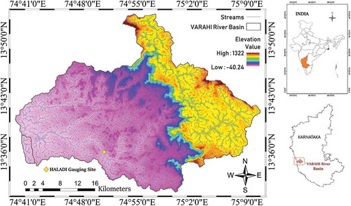
The precipitation data of 04 grid points falling within the Varahi basin derived from the new high spatial resolution (0.25° × 0.25°) daily gridded rainfall dataset (Pai et al. 2014) for the years 1986 to 2012 were used in the study. The Thiessen Polygon method was used under GIS platform to extract or compute the areal average precipitation over the Varahi basin. Similarly, the CHIRPS satellite based precipitation product (Funk et al. 2015) of spatial resolution 0.05° over the Varahi river basin was extracted using Google Earth Engine tool (Gorelick et al. 2017) for the years 1986 to 2012. The data statistics, namely, maximum, minimum, mean, standard deviation, coefficient of variation, skewness and kurtosis of streamflow, precipitation derived from IMD and CHIRPS precipitation data are tabulated in Table 1. For modeling, the overall data was divided into training and testing dataset. The data of the period 01/01/1986 and 31/12/2005 was considered for the training of ML models and the data of the period from 01/01/2006 to 31/12/2012 was considered for model testing. Very high variability could be observed in CHIRPS precipitation data of both train and test phase compared to that of IMD precipitation data. In the case of streamflow, the maximum discharge could be seen in the testing data. The train and test phase standard deviation of streamflow data were nearly analogous to each other.

Table 1. Descriptive statistics of daily scale precipitation and streamflow data of Haladi gauging station in Varahi river

Statistics	Min	Max	Mean	STD	CV	Skewness	Kurtosis
Train Dataset
IMD Precipitation Data (mm)	0.00	240.30	10.97	21.72	1.98	3.12	12.91
CHIRPS Precipitation Data (mm)	0.00	409.04	8.84	30.89	3.49	5.88	44.33
Streamflow Data (cumec)	0.00	915.80	58.55	85.06	1.45	3.33	14.85
Test Dataset
IMD Precipitation Data (mm)	0.00	297.78	14.01	28.09	2.01	3.02	11.99
CHIRPS Precipitation Data (mm)	0.00	326.34	10.68	26.48	2.48	4.01	22.70
Streamflow Data (cumec)	0.15	1003.65	69.39	85.27	1.23	3.53	17.92

Min – Minimum; Max – Maximum; STD – Standard Deviation; CV – Coefficient of Variation.

3 Theoretical overview of machine learning paradigms

3.1 Group method of data handling

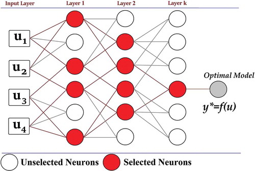
By automatically detecting the cross-correlations that exist between various data subsets, Group Method of Data Handling (GMDH) algorithms find an optimal model structure or network to incrementally increase the accuracy of learning and predictions (Ivakhnenko and Ivakhnenko 1995). A set of several efficient algorithms constitutes Group Method of Data Handling framework for adaptive and supervised learning of non-linear and probabilistic functions. Well-defined principles of self-organization, assists GMDH to robotically determine the optimal number of hidden layers and their neurons along with other associated hyper-parameters of the network to minimize the prediction error criteria (Onwubolu 2016). In a time-series regression task of multiple inputs and a single output, the GMDH constructs a subset of high order polynomial function:

(1) $Y\left(x_1,\dots .\dots .,x_n\right)=p+{\sum }_{i=1}^n{q}_i\cdot x_i+{\sum }_{i=1}^n{\sum }_{j=1}^n{r}_{ij}{x}_i{x}_j+{\sum }_{i=1}^n{\sum }_{j=1}^n{\sum }_{k=1}^n{s}_{ijk}{x}_i{x}_j{x}_k+\dots \dots .$(1)

where, (p, q, r, s, … .) denotes the vector of variable coefficients/weights in the polynomial; “n” denotes number of polynomial function components. Here, x are inputs, Y is the output or response variable. Each node/neuron of the multilayer GMDH network (Fig. 2) is fed with bivariate activation polynomials whose output are again fed forward to post layers of the network to arrive at partial polynomial models. This cycle/process continues until a single neuron is sort-out in the last layer. The coefficients (p, q, r, s, … …) of the polynomials are calculated by fitting least square algorithm. The Ivakhnenko polynomial ($i_p$) of the form $i_p\left(x_1,x_2\right)={\alpha }_0+{\alpha }_1{x}_1+{\alpha }_2{x}_2+{\alpha }_3{x}_1{x}_2+{\alpha }_4{x}_1^2+{\alpha }_5{x}_2^2$ is used to derive the output of each neuron. The number of partial polynomial models so constructed determine the complexity of the model. The selected neurons in each layer are the optimal ones sorted out based on any external criteria of accuracy. The neuron with minimal/least regularity criterion in the end layer will be the final output of the GMDH network. For further detailed information on GMDH network architecture and its implementation refer to Farlow (1984), Anastasakis and Mort (2001) and Dag and Yozgatligil (2016).

Figure 2. GMDH network architecture

3.2 Chi-square automatic interaction detector

Kass (1980) formulated Chi-square Automatic Interaction Detector (CHAID) trees that use Person’s Chi-square tests of independence to check for interrelation or association between input and output variables without making any assumptions from the underlying data. The standard methodological approach of the CHAID algorithm involves recursive partitioning to construct an optimal tree structure by identifying a split condition at each (non-terminal) node that reduces uncertainty in the predicted response variable based on its correspondence with a set of independent/splitting variables. Initially, the relevant independent variables identified are sorted hierarchically in such a way that the variable with lowest p-value becomes the first independent variable for the partition due to its strong association with the response variable (Milanovic and Stamenkovic 2016). The simple workflow of CHAID tree includes merging, multiway splitting, and stopping steps. In regression tasks, the dependent variable is often continuous and hence, at each step an F test is run to determine the next best split at a node based on the significance criterion. By optimally merging all splitting variables, CHAID curtails the over-fitting problem. CHAID tree stops growing when met with any one of the following stopping criterion. Firstly, when the user-defined maximum number of tree levels are reached; secondly, when the parent node size falls less than the user-defined minimum node size, CHAID fails to split a node; thirdly, when a node is split as a child node whose size falls less than the user-defined minimum child node size, again the CHAID ends in a terminal; and lastly, the CHAID fails to split a node when the split threshold (p-value) is above the significance level (0.05) (Ritschard 2013). For details of computational issues, tree building procedures of CHAID one can refer to Statsoft (2020) and van Diepen and Franses (2006).

3.3 Random forests

Random Forests (RF) belong to the class of supervised machine learning algorithms that associate multiple randomized decision trees and ensemble their predictions by averaging to provide better predictive results of good generalization along with no over-fitting problem (Breiman 2001). Their mechanism is versatile enough even for complex regression tasks. Consider a nonparametric regression task, which aims to predict the square integrable random response $Y\in \mathrm{{\rm Y}}$ by employing a regression function $m\left(x\right)=E\left[Y|X=x\right]$ using an observed input random vector $X\in {\left[0,1\right]}^P$. The regression function estimate $m_n:{\left[0,1\right]}^p\to \mathrm{{\rm Y}}$ is constructed by using training sample of independent random variables $D_n=\left(X_1,Y_1\right),\dots \dots \dots ,\left(X_n,Y_n\right)$ which have an identical distribution to that of an independent prototype pair (X, Y). The function m estimate is regarded to be consistent if it satisfies the condition, $E{\left[m_n\left(x\right)-m\left(x\right)\right]}^2\to 0$ (mean squared error) as $n\to \mathrm{\infty }$. As already mentioned RF uses the technique of bootstrap aggregating of randomized decision trees. Hypothetically, prior to growing of individual trees, a variable Θ resamples the train set to select the new directions for splitting, thus making the trees de-correlated and pruned by a stopping criteria. After training, by averaging the predictions of all individual trees a (finite) forest estimate for unseen samples is made:

(2) $m_{M,n}\left(x,{\mathrm{\Theta }}_1,\dots .\dots ..,{\mathrm{\Theta }}_M,D_n\right)=\frac{1}{M}\sum _{j=1}^M{m}_n\left(x;{\mathrm{\Theta }}_j,D_n\right)$(2)

where, M is the number of trees in the forest that are chosen arbitrarily (Scornet 2015). The RF reduces the average error of the trees with the use of a factor $\bar{\rho }$

(3) $\bar{\rho }=\frac{E_{\mathrm{\Theta }}{E}_{\mathrm{\Theta }{ }^{\mathrm{\prime }}}\left[\rho \left(\mathrm{\Theta },\mathrm{\Theta }{ }^{\mathrm{\prime }}\right)\cdot sd\left(\mathrm{\Theta }\right)\cdot sd\left(\mathrm{\Theta }{ }^{\mathrm{\prime }}\right)\right]}{{\left[E_{\mathrm{\Theta }}sd\left(\mathrm{\Theta }\right)\right]}^2}$(3)

where, $\bar{\rho }$ is mean correlation value, $\rho \left(\mathrm{\Theta },\mathrm{\Theta }{ }^{\mathrm{\prime }}\right)$ is the correlation between raw margin functions holding $\mathrm{\Theta }$, $\mathrm{\Theta }{ }^{\mathrm{\prime }}$ and $sd\left(\mathrm{\Theta }\right)$ is the standard deviation of raw margin function. The advantages of Random Forests include high accuracy results, no over-fitting problem, works even with missing values in the dataset, invariant to monotonic transformations of the input variables. For additional information on Random forests one can refer to Pavlov (2000), Louppe (2014) and Biau and Scornet (2016).

4 Intrinsic time-scale decomposition

Intrinsic Time-scale Decomposition (ITD) has grabbed considerable attention nowadays owing to its robustness in time–frequency–energy (TFE) analysis of nonlinear or nonstationary data. The ITD algorithm starts by analyzing a signal’s intrinsic timescale components, namely, the signal’s extreme points (maximum and minimum) and any other critical points before decomposing a time-series data or signal into a set of sequentially lower frequency components. This self-extraction process iterates to sort out even the smallest remaining (high frequency) timescale modes in successive steps from baseline (lower frequency) signals. The last iterated mode corresponds to the largest timescale embedded in the signal which is generally referred to as “monotonic trend” (Frei and Osorio 2006). A nonlinear time-series signal (P_t) is decomposed as,

(4) $P_t=\lambda P_t+\left(1-\lambda \right)P_t=L_t+H_t$(4)

where, $\lambda$ is a factor that extracts a baseline signal $L_t=\lambda P_t$ from P_t along with proper rotation component $H_t=\left(1-\lambda \right)P_t$

Initially, ITD analysis identifies P_k, the local extrema of P_t occurring at time instant ${\tau }_k$, (k = 1, 2, …) while assuming ${\tau }_0=0$. Considering, L_t and H_t over the interval [0; ${\tau }_k$], and P_t being available for $t\in \left[0,{\tau }_{k+2}\right]$, a baseline signal over the interval $\left({\tau }_k,{\tau }_{k+1}\right)$ is derived using piece-wise linear extraction factor between the successive extrema P_k and P_k+1 as:

(5) $\lambda P_t=L_t=L_k+\frac{\left(L_{k+1}-L_k\right)}{\left(P_{k+1}-P_k\right)}\left(P_t-P_k\right);t\in \left[{\tau }_k,{\tau }_{k+1}\right]$(5)

where,

(6) $L_{k+1}=\alpha \left[P_k+\left(\frac{{\tau }_{k+1}-{\tau }_k}{{\tau }_{k+2}-{\tau }_k}\right)\left(P_{k+2}-P_k\right)\right]+\left(1-\alpha \right)P_{k+1};0<\alpha <1$(6)

Using a proper-rotation-extracting operator, $\mathcal{H}$, the first proper rotation is extracted from P_t as:

(7) $\mathcal{H}{P}_t\equiv \left(1-\lambda \right)P_t=H_t=P_t-L_t$(7)

Using the baseline signals as input, the above steps iterates until a monotonic baseline signal is established. Finally, a raw time-series signal decomposed using ITD yields a sequence of proper rotation components (PRC) and a monotonic trend:

(8) $P_t=\mathcal{H}{P}_t+\lambda P_t=\mathcal{H}{P}_t+\left(\mathcal{H}+\lambda \right)\lambda P_t=\left(\mathcal{H}\left(1+\lambda \right)+{\lambda }^2\right)P$(8)

(9) $=\left(\mathcal{H}\sum _{k=0}^{n-1}{\lambda }^k+{\lambda }^n\right)P_t$(9)

where, $\mathcal{H}{\lambda }^k{P}_t$ is the (k + 1)^st level proper rotation and ${\lambda }^n{P}_t$ is the monotonic trend. It is suggested to refer to Frei and Osorio (2007) for detailed information on the mathematical aspects of ITD.

5 Model development and performance evaluation

For calibrating ML models, the input variables were determined based on the magnitude of cross correlation between the lags of precipitation and streamflow time-series data (Fig. 3). Considering one, three and seven days ahead streamflow time-series as the dependent/response variables, the lagged time-series of IMD/CHIRPS rainfall and streamflow were pondered as the predictor variables for ML models.

Figure 3. ACF, PACF and CCF of rainfall data products and streamflow data

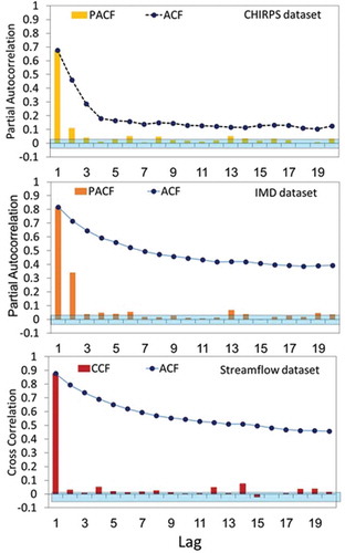
The input-output structure of ML models using IMD rainfall data:

$P_{\left(t-2\right)}+P_{\left(t-1\right)}+P_{\left(t\right)}+Q_{\left(t-1\right)}+Q_{\left(t\right)}\to Q_{\left(t+1\right)}/Q_{\left(t+3\right)}/Q_{\left(t+7\right)}$

The input-output structure of ML models using CHIRPS rainfall data:

$P_{\left(t-1\right)}+P_{\left(t\right)}+Q_{\left(t-1\right)}+Q_{\left(t\right)}\to Q_{\left(t+1\right)}/Q_{\left(t+3\right)}/Q_{\left(t+7\right)}$

where, P represents either IMD/CHIRPS rainfall time-series, Q denotes the streamflow time series.

The model parameter settings used to calibrate GMDH models include maximum number of layers in the range 2–8, maximum number of neurons in a layer in the range 5–20, selection pressure (α) = 0.05, and number of loops = 100. The CHAID models were run with parent nodes in the range 5–100, V-fold cross validation set at 10 folds and significance set at (α_split, α_merge, and p value) ≤ 0.05. The Random Forest regressor was built using the bag and batch size in the range 80–120, maximum depth = 3, criterion to measure the quality of split set as mean squared error (MSE), bootstrap = True and minimum number of samples required to split an internal node was set = 2. In order to improve the forecast accuracy, Intrinsic Time-Scale Decomposition was introduced as the data preprocessing technique. The streamflow and IMD/CHIRPS rainfall data time-series were decomposed into five proper rotation components (PRC) and a monotonic trend. An example of the ITD decomposed streamflow data is presented in Fig. 4. The methodology flowchart is presented in Fig. 5.

Figure 4. ITD decomposition of streamflow data into PRC’s and the residual

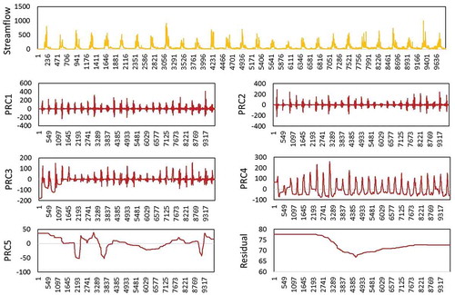
Figure 5. Methodology workflow of standalone and ITD hybridized ML model development for multi-step lead-time streamflow forecasting. [GMDH: Group Method of Data Handling; CHAID: Chi-square Automatic Interaction Detector; RF: Random Forests; ITD: Intrinsic Time-scale Decomposition; PRC: Proper Rotation Components; Res: Residuals]

The multi-step ahead streamflow forecasts were evaluated using both error and efficiency statistics. The statistical model evaluation metrics (Yaseen et al. 2020) employed to assess the model performances are listed below.

1. Normalized Nash-Sutcliffe Efficiency (NNSE)

(10) $NNSE=\frac{1}{\left(2-NSE\right)}$(10)

(11) $NSE=1-\frac{{\sum }_{x=1}^N{\left(O_x-P_x\right)}^2}{{\sum }_{x=1}^N{\left(O_x-\bar{O}\right)}^2}$(11)

• (2) Root Mean Square Error (RMSE)

(12) $RMSE=\sqrt{\frac{{\sum }_{x=1}^N{\left(O_x-P_x\right)}^2}{N}}$(12)

• (3) Percent Bias (PBias)¹

(13) $PBias=\left(\frac{{\sum }_{x=1}^N\left(P_x-O_x\right)}{{\sum }_{x=1}^N{O}_x}\right)\times 100$(13)

• (4) Kling-Gupta Efficiency (KGE)

(14) $KGE=1-\sqrt{{\left(R-1\right)}^2+{\left(\beta -1\right)}^2+{(\gamma -1)}^2}$(14)

(15) $R=\left[\frac{{\sum }_{x=1}^N\left(O_x-\bar{O}\right)\cdot \left(P_x-\bar{P}\right)}{\sqrt{{\sum }_{x=1}^N{\left(O_x-\bar{O}\right)}^2\cdot {\sum }_{x=1}^N{\left(P_x-\bar{P}\right)}^2}}\right]$(15)

(16) $\beta =\frac{\bar{P}}{\bar{O}}$(16)

(17) $\gamma =\frac{C{V}_P}{C{V}_O}=\frac{{\sigma }_P/\bar{P}}{{\sigma }_O/\bar{O}}$(17)

where, O is the observed values; P is the model computed values; $\bar{O}$ is the mean of observed values; $\bar{P}$ is the mean of model computed values; ${\sigma }_O$ and ${\sigma }_P$ are the standard deviation of observed and model computed values, respectively; CV_O and CV_P are the coefficient of variation of observed and model computed values, respectively; and N is the number of data points.

6 Results and discussion

The actual streamflow time series of Haladi gauging site were modeled by using GMDH, CHAID and RF models fed with distinct input-output (i/o) data combinations. The antecedent daily precipitation and streamflow data (in the form of lags) were employed as the inputs in order to model one, three and seven days ahead streamflow. The statistical measures computed by using the actual versus forecasted streamflow values of standalone ML and ITD hybridized ML models were comparatively evaluated. The computational costs required for training of standalone ML models are presented in Table 2.

Table 2. Computational costs of the proposed standalone models at all lead-time periods

Forecast Horizon	GMDH (Seconds)	CHAID (Seconds)	RF (Seconds)
Q(t+1)	3.68	1.92	1.54
Q(t+3)	3.92	2.16	1.93
Q(t+7)	3.95	2.48	1.91

6.1 One-day lead time streamflow forecasting

The performance of standalone and ITD hybridized GMDH, CHAID and RF models calibrated by using antecedent IMD rainfall and streamflow data as inputs are tabulated in Table 3. Here, the results demonstrate that, in one day ahead streamflow (Q_(t+1)) forecasting, the ITD-RF model performed relatively superior to that of other ITD hybridized and standalone ML models with test phase KGE = 0.885 and RMSE = 38.707 cumec.² Among standalone ML models, the GMDH model provided fairly less biased one-day lead-time streamflow forecasts with test phase KGE = 0.845 and RMSE = 44.083 cumec. Interestingly, the GMDH model forecasts were least biased (Test PBias = 0.394) in contrast to other forecasts. The Table 4 presents the performance statistics of standalone and ITD hybridized GMDH, CHAID and RF models calibrated by using antecedent CHIRPS rainfall and streamflow data as inputs. It is quite apparent from this table that again the ITD-RF model performed well in forecasting one day ahead streamflows with test phase KGE = 0.914 and RMSE = 32.818 cumec. However, the PBias = −2.702 indicates an over-estimation of actual values. On comparison of data from this Table 4 with that of in Table 3, it is evident that the ML models developed using CHIRPS rainfall and streamflow data as inputs showed relatively superior performance to that of models developed using IMD rainfall and streamflow data.

Table 3. Performance of standalone and ITD hybridized GMDH, CHAID and RF models using antecedent IMD precipitation and streamflow data as input attributes (1, 3 & 7 days lead time)

Models		GMDH	CHAID	RF	ITD-GMDH	ITD-CHAID	ITD-RF
Q(t+1) Models
KGE	TRAIN	0.841	0.873	0.859	0.855	0.893	0.945
	TEST	0.845	0.769	0.844	0.827	0.869	0.885
NNSE	TRAIN	0.824	0.852	0.84	0.838	0.894	0.974
	TEST	0.791	0.692	0.78	0.805	0.816	0.829
RMSE (cumec)	TRAIN	39.206	35.521	37.038	37.462	29.398	13.948
	TEST	44.083	56.884	45.27	42.017	40.531	38.707
PBias	TRAIN	0	−9.441	−0.005	−1.637	0.06	−0.573
	TEST	0.394	−7.961	−0.774	1.421	−2.79	−4.822
Q(t+3) Models
KGE	TRAIN	0.666	0.661	0.724	0.81	0.84	0.907
	TEST	0.61	0.578	0.623	0.714	0.723	0.769
NNSE	TRAIN	0.708	0.72	0.668	0.806	0.82	0.95
	TEST	0.668	0.543	0.68	0.696	0.712	0.722
RMSE (cumec)	TRAIN	54.582	53.057	59.926	41.762	39.796	19.662
	TEST	60.11	78.248	58.486	56.349	54.166	52.954
PBias	TRAIN	−0.21	12.715	−6.708	−3.685	−3.594	−1.664
	TEST	3.882	−7.521	13.523	1.236	−2.758	−5.718
Q(t+7) Models
KGE	TRAIN	0.459	0.59	0.645	0.576	0.594	0.704
	TEST	0.443	0.587	0.457	0.553	0.57	0.726
NNSE	TRAIN	0.618	0.632	0.671	0.646	0.657	0.758
	TEST	0.602	0.582	0.6	0.609	0.637	0.701
RMSE (cumec)	TRAIN	66.911	64.850	59.534	62.992	61.416	48.028
	TEST	69.333	72.275	69.627	68.336	64.36	55.626
PBias	TRAIN	0	18.947	−2.562	0	0.053	−0.406
	TEST	4.858	−4.578	19.158	2.018	1.37	−7.733

Table 4. Performance of standalone and ITD hybridized GMDH, CHAID and RF models using antecedent CHIRPS precipitation and streamflow data as input attributes (1, 3 & 7 days lead time)

Models		GMDH	CHAID	RF	ITD-GMDH	ITD-CHAID	ITD-RF
Q(t+1) Models
KGE	TRAIN	0.871	0.878	0.905	0.849	0.897	0.941
	TEST	0.824	0.84	0.833	0.822	0.854	0.914
NNSE	TRAIN	0.852	0.855	0.901	0.887	0.889	0.972
	TEST	0.794	0.804	0.803	0.821	0.829	0.871
RMSE (cumec)	TRAIN	35.468	34.928	28.197	30.398	30.063	14.412
	TEST	43.444	42.087	42.251	39.838	38.689	32.818
PBias	TRAIN	−7.068	−0.231	−1.476	−11.386	−1.529	−0.476
	TEST	−4.406	−0.573	−0.436	−9.537	−1.302	−2.702
Q(t+3) Models
KGE	TRAIN	0.729	0.73	0.907	0.807	0.877	0.893
	TEST	0.666	0.661	0.682	0.786	0.839	0.85
NNSE	TRAIN	0.669	0.745	0.901	0.846	0.858	0.95
	TEST	0.597	0.681	0.697	0.794	0.816	0.821
RMSE (cumec)	TRAIN	59.834	49.827	28.167	36.286	34.584	19.535
	TEST	69.975	58.335	56.148	43.44	40.514	39.843
PBias	TRAIN	7.527	−0.102	−1.819	−13.34	−1.921	−0.689
	TEST	9.644	−1.117	−0.991	−11.193	−1.466	−2.382
Q(t+7) Models
KGE	TRAIN	0.678	0.676	0.876	0.808	0.83	0.862
	TEST	0.582	0.558	0.581	0.76	0.775	0.788
NNSE	TRAIN	0.686	0.712	0.861	0.806	0.808	0.936
	TEST	0.62	0.627	0.642	0.777	0.785	0.799
RMSE (cumec)	TRAIN	57.508	54.125	34.159	41.754	41.406	22.099
	TEST	66.737	65.745	63.609	45.648	44.629	42.763
PBias	TRAIN	−1.809	−0.419	−1.543	−3.624	−1.523	−0.626
	TEST	0.047	−1.111	−1.128	−3.381	−0.264	−0.661

6.2 Three days ahead streamflow forecasting

With regard to three days ahead streamflow(Q_(t+3)) forecasting, essentially the same Tables 3 and 4 convey the performance statistics of standalone and ITD hybridized GMDH, CHAID and RF models. Overall, the ITD-RF model was the one that obtained the most satisfactory results. The RMSE of ITD-RF model developed using CHIRPS rainfall and streamflow data as input attributes reduced by 24.75% in contrast to ITD-RF model developed using IMD rainfall and streamflow data as input attributes. Generally, if PBias ≤ ±20, the modeled forecasts are considered to be good. The generalization and forecast efficiencies of standalone ML models were relatively low with higher RMSE. Specifically, the CHAID model fed with IMD rainfall and streamflow data as input attributes provided poor forecasts with NNSE = 0.543 and RMSE = 78.248 cumec during the test phase. The ITD hybridized ML models presented much better performance owing to decomposition of data that accounts for several components of a time series (usually a trend, periodic and random components). For example, the ITD-CHAID model fed with ITD decomposed IMD rainfall and streamflow data as input attributes yielded improved streamflow forecasts with test phase NNSE = 0.712 and RMSE = 54.166 cumec; the usage of ITD decomposed data led to the reduction of RMSE by almost 30.77% and increase in NNSE by 31.12%. However, even better results were achieved by ML models using ITD decomposed CHIRPS rainfall and streamflow data as input attributes.

6.3 Seven days ahead streamflow forecasting

For producing reliable long-range forecasts/projections, the ML models often encounter difficulty in learning complex data within non-stationary environments. In line with previous sections, the Tables 3 and 4 portray the performance indices of standalone and ITD hybridized GMDH, CHAID and RF models calibrated for yielding a week lead-time streamflow forecasts. The standalone ML models fed with either IMD/CHIRPS rainfall and streamflow data as input attributes provided poor seven days ahead streamflow forecasts with test phase NNSE ≤ 0.642 and RMSE ≥ 63.609 cumec. This research verified that using ITD decomposed data in ML models significantly improves the long-range streamflow forecasts. For instance, the ITD-RF model (fed with CHRIPS rainfall and streamflow data as input attributes) provided relatively satisfactory streamflow forecasts with test phase NNSE = 0.799, RMSE = 42.763 cumec and PBias = −0.661. Likewise, the other forecast performances of ITD-GMDH and ITD-CHAID models were broadly in line with that of ITD-RF model results with test phase NNSE = 0.777 and 0.785, respectively. The results confirm that ITD enhances the learning capability of ML models by attribute set decomposition that generalizes the task of significant feature selection from the dataset. The inherent instantaneous amplitude and phase information embedded in complex and non-stationary time-series data is extracted and utilized in ITD to enhance the time-frequency resolution of data besides preserving its precise temporal information (Frei and Osorio 2007).

6.4 Comparative evaluation of standalone and ITD hybridized ML models

It is interesting to note that at all three forecast horizons of this study, the ITD-RF models were comparatively superior to others. In the case of ITD-RF models that use IMD rainfall and streamflow data as input attributes, the forecast efficiencies at three and seven days lead-time decreases by 13.10% and 17.96% as per KGE metric with reference to one day ahead streamflow forecasts. Superior results were seen in ITD-RF models that use CHIRPS rainfall and streamflow data as input attributes wherein the forecast efficiencies at three and seven days lead-time decreases by 07% and 15.97% as per KGE metric with reference to one day ahead streamflow forecasts. Additionally, the RMSE of ITD-RF models fed with CHIRPS rainfall and streamflow data as input attributes reduced by 15.21%, 24.75% and 23.12% at one, three and seven days forecast horizons, respectively, with reference to that of ITD-RF models fed with IMD rainfall and streamflow data as input attributes.

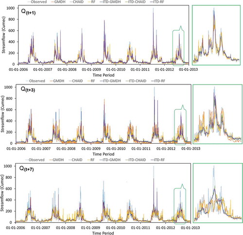
The Figs. 6 and 7 portray the line plots of observed versus forecasted daily streamflow time-series of the ITD hybridized ML models and their corresponding standalone ones of the test time-period. Multiple time-series plots of different forecast horizon together in the same figure depict the capabilities of each standalone and ITD hybridized ML models in generating unbiased estimates of daily streamflow time series taking into account of random and seasonal patterns. The one-day lead-time ITD-RF model estimates are seen to almost certainly catch/capture the cyclic, irregular, random and extreme variations of the observed daily streamflow time-series.

Figure 6. Plots of daily streamflow time series modeled via standalone and ITD hybridized ML models (calibrated using IMD precipitation data) against the observed streamflow time-series of test phase

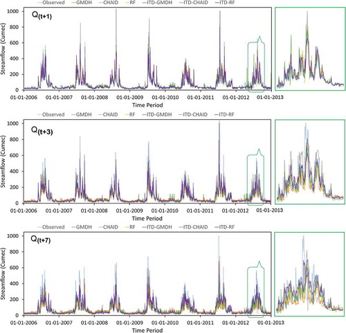
Figure 7. Plots of daily streamflow time series modeled via standalone and ITD hybridized ML models (calibrated using CHIRPS precipitation data) against the observed streamflow time-series of test phase

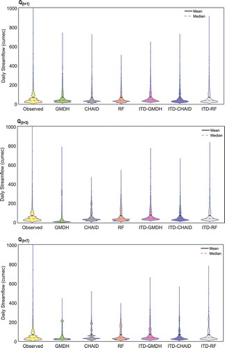
Violin plot offers the dual advantage of a box plot and a kernel density plot. The Figs. 8 and 9 portray the Violin plots of observed and forecasted daily streamflow time-series of the standalone and ITD hybridized ML models of the test time-period. Violin plots illustrate summary statistics as box plots with central red dotted lines representing the median value of time-series, the thick black lines inside the violin envelope representing the interquartile range and understanding the violin shape is exactly similar to a density plot: that shows the frequency distribution of the data. Referring to Figs. 8 and 9, it’s very clear that there is changing variability in modeled streamflow time-series data; the variability is much higher at the peaks. The extreme peak values are underestimated by almost all the models.

Figure 8. Violin plots for comparison of observed streamflow time-series of test phase with that of modeled ones using standalone and ITD hybridized ML models calibrated using IMD precipitation data

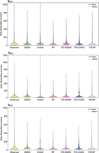
Figure 9. Violin plots for comparison of observed streamflow time-series of test phase with that of modeled ones using standalone and ITD hybridized ML models calibrated using CHIRPS precipitation data

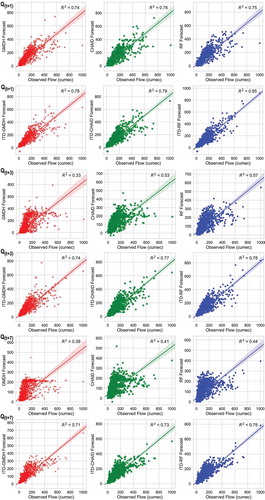
The Figs. 10 and 11 depict the scatter plots of observed versus forecasted daily streamflow time series of the standalone and ITD hybridized ML models of the test time-period. Closer inspection of Fig. 10 reveals that the forecasted streamflow data from ML models of seven days lead-time (Q_(t+7)) were widely spread and have a more number of outliers indicating a relatively weak relationship with the actual streamflow data. Barring few outliers, majority of the forecasted streamflow values (Fig. 11) of ITD-RF model was closely spread within the confidence band showing a significant relationship with the observed streamflow data of test time-period.

Figure 10. Scatter plots of observed versus forecasted streamflow time-series of test phase with respect to standalone and ITD hybridized ML models calibrated using IMD precipitation data

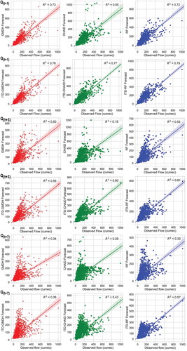
Figure 11. Scatter plots of observed versus forecasted streamflow time-series of test phase with respect to standalone and ITD hybridized ML models calibrated using CHIRPS precipitation data

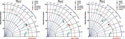
The forecast performance or the relative skill of different standalone and ITD hybridized ML models are graphically summarized via Taylor diagrams (Taylor 2001) as presented in Figs. 12 and 13. In Taylor diagram, each colored point/dot represents the testing performance of individual models. Three statistical indices, namely the correlation coefficient (R), the standard deviation ($\sigma$) and the (centered) root-mean-square difference (RMSD) characterize the statistical relationship between the modeled and reference fields. From the Taylor diagrams in Figs. 12 and 13, it is evident that the ITD-RF model forecasts best fits all the one, three and seven days ahead streamflow time series and has a standard deviation close to that of actual streamflow time-series. These diagrams clearly depict the high forecast skill of ITD hybridized ML models in forecasting one-day lead time (Q_(t+1)) streamflow time-series, however, the seven-day lead-time forecasts (Q_(t+7)) from the same models showed distorted standard deviations compared to that of the actual streamflow time series.

Figure 12. Taylor diagram depicting test phase performance of standalone and ITD hybridized ML models calibrated using IMD precipitation data

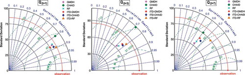
Figure 13. Taylor diagram depicting test phase performance of standalone and ITD hybridized ML models calibrated using CHIRPS precipitation data

The reported statistical results validate the adopted research hypothesis on the utilization of CHIRPS (satellite derived) precipitation data as a product for streamflow process generation. In addition, there exists significant improvement in the forecast performance of the newly introduced hybrid ML models (i.e. ITD-GMDH, ITD-CHAID and ITD-RF) through the integration with ITD approach. The research findings evidenced the correlation of CHIRPS precipitation data for the streamflow forecasting; along with, the prospective of data preprocessing using the ITD approach. Additionally, the results confirmed the applicability of the proposed methodology for the three advanced time horizons (one, three and seven). This is highly essential for sustainable water resources engineering, which includes both planning and management. The current research can be further extended to validate the current results with some well-established ML models over the literature such as extreme learning machine, support vector machine, adaptive neuro fuzzy inference system, etc. In addition, investigate the potential of the proposed data-intelligence scheme for other case study (different region) to confirm the generalization capacity of the methodology.

7 Conclusions

The prime objective of this research was to evaluate the applicability of CHIRPS precipitation data for multi-step ahead daily streamflow forecasting of Varahi river gauged at Haladi station near Kundapura, India using standalone and ITD hybridized ML models. On the basis of the results obtained the following conclusions are drawn out of this study. The satellite derived CHIRPS precipitation data product was useful in simulating robust streamflow forecasting models which were much superior to models incorporating IMD rainfall data source over of the Varahi river basin. The ML models were susceptible to the rainfall data product source and input-output combinations used. The findings of this study boosts the confidence to use the CHIRPS rainfall data for hydrologic modeling applications. ITD enhances the time-frequency resolution of time-series data besides preserving its precise temporal information. The hybrid ML modeling strategies that include intrinsic time-scale decomposition (ITD) as a pre-processing tool are fully scalable and therefore can be applied to model any hydrological parameter of interest. The performance indices reflect that ITD-RF model produced promising one, three and seven days ahead streamflow forecasts. The model performance evaluation schemes such as Taylor diagrams substantially assist in distinguishing the model skills. A further study could comparatively evaluate the application of CHIRPS and other satellite precipitation products in streamflow forecasting over the basins of contrasting climatic conditions.

CRediT author statement

(1) Maofa Wang: Methodology; Software; Data analysis; Model Development; Validation.

(2) Mohammad Rezaie-Balf: Conceptualization; Methodology; Software; Data analysis; Model Development.

(3) Sujay Raghavendra Naganna: Conceptualization; Writing - Original draft, Editing & Reviewing; Visualization; Formal analysis; Supervision.

(4) Zaher Mundher Yaseen: Writing - Editing & Reviewing; Supervision.

Acknowledgements

The authors wish to acknowledge the India-WRIS WebGIS module, Ministry of Jal Shakti and Indian Meteorological Department of Government of India for providing the necessary data required for research.

Disclosure statement

No potential conflict of interest was reported by the author(s).

Additional information

Funding

This research received no external funding.

Notes

¹ Note: The optimal value of PBIAS is zero (0). “+” values indicate overestimation bias, and “–” values indicate underestimation bias.

² Note: cumec = cubic meter per second (m³/s), SI unit of rate of flow of water.

References

- Adamowski, J. and Sun, K., 2010. Development of a coupled wavelet transform and neural network method for flow forecasting of non-perennial rivers in semi-arid watersheds. Journal of Hydrology, 390 (1–2), 85–91. doi:10.1016/j.jhydrol.2010.06.033
- Adnan, R.M., et al., 2020. Least square support vector machine and multivariate adaptive regression splines for streamflow prediction in mountainous basin using hydro-meteorological data as inputs. Journal of Hydrology, 586, 124371. doi:10.1016/j.jhydrol.2019.124371
- Adnan, R.M., et al., 2019. Daily streamflow prediction using optimally pruned extreme learning machine. Journal of Hydrology, 577, 123981. doi:10.1016/j.jhydrol.2019.123981
- Anastasakis, L. and Mort, N., 2001. The development of self-organization techniques in modelling: a review of the Group Method of Data Handling (GMDH). UK: Department of Automatic Control & Systems Engineering, The University of Sheffield, Tech. Rep. 813.
- Ashouri, H., et al., 2015. PERSIANN-CDR: daily precipitation climate data record from multisatellite observations for hydrological and climate studies. Bulletin of the American Meteorological Society, 96 (1), 69–83. doi:10.1175/BAMS-D-13-00068.1
- Band, S.S., et al., 2020. Flash flood susceptibility modeling using new approaches of hybrid and ensemble tree-based machine learning algorithms. Remote Sensing, 12 (21), 3568. doi:10.3390/rs12213568
- Beck, H.E., et al., 2017a. MSWEP: 3-hourly 0.25 global gridded precipitation (1979–2015) by merging gauge, satellite, and reanalysis data. Hydrology and Earth System Sciences, 21 (1), 589–615. doi:10.5194/hess-21-589-2017
- Beck, H.E., et al., 2017b. Global-scale evaluation of 22 precipitation datasets using gauge observations and hydrological modeling. Hydrology and Earth System Sciences, 21 (12), 6201. doi:10.5194/hess-21-6201-2017
- Biau, G. and Scornet, E., 2016. A random forest guided tour. Test, 25 (2), 197–227. doi:10.1007/s11749-016-0481-7
- Breiman, L., 2001. Random forests. Machine Learning, 45 (1), 5–32. doi:10.1023/A:1010933404324
- Chiang, Y.M., Chang, L.C., and Chang, F.J., 2004. Comparison of static-feedforward and dynamic feedback neural networks for rainfall–runoff modeling. Journal of Hydrology, 290 (3–4), 297–311. doi:10.1016/j.jhydrol.2003.12.033
- Cloke, H. and Pappenberger, F., 2009. Ensemble flood forecasting: a review. Journal of Hydrology, 375 (3–4), 613–626. doi:10.1016/j.jhydrol.2009.06.005
- Dag, O. and Yozgatligil, C., 2016. GMDH: an R package for short term forecasting via GMDH-type neural network algorithms. The R Journal, 8 (1), 379–386. doi:10.32614/RJ-2016-028
- Di, C., Yang, X., and Wang, X., 2014. A four-stage hybrid model for hydrological time series forecasting. PloS One, 9 (8), e104663. doi:10.1371/journal.pone.0104663
- Famili, A., et al., 1997. Data preprocessing and intelligent data analysis. Intelligent Data Analysis, 1 (1), 3–23. doi:10.3233/IDA-1997-1102
- Farlow, S.J., 1984. Self-organizing methods in modeling: GMDH type algorithms, Statistics: Textbooks and Monographs, Vol. 54. New York: Marcel Dekker.
- Frei, M.G. and Osorio, I., 2006. Method, computer program, and system for intrinsic timescale decomposition, filtering, and automated analysis of signals of arbitrary origin or timescale, Available from: https://patents.google.com/patent/US7054792/en, US Patent 7054792B2.
- Frei, M.G. and Osorio, I., 2007. Intrinsic time-scale decomposition: time–frequency–energy analysis and real-time filtering of non-stationary signals. Proceedings of the Royal Society A: Mathematical, Physical and Engineering Sciences, 463 (2078), 321–342. doi:10.1098/rspa.2006.1761
- Fu, M., et al., 2020. Deep learning data intelligence model based on adjusted forecasting window scale: application in daily streamflow simulation. IEEE Access, 8, 32632–32651. doi:10.1109/ACCESS.2020.2974406
- Funk, C., et al., 2015. The climate hazards InfraRed precipitation with stations—a new environmental record for monitoring extremes. Scientific Data, 2 (1), 1–21. doi:10.1038/sdata.2015.66
- Gautam, D. and Holz, K.P., 2001. Rainfall-runoff modelling using adaptive neuro-fuzzy systems. Journal of Hydroinformatics, 3 (1), 3–10. doi:10.2166/hydro.2001.0002
- Gorelick, N., et al., 2017. Google earth engine: planetary-scale geospatial analysis for everyone. Remote Sensing of Environment, 202, 18–27. doi:10.1016/j.rse.2017.06.031
- Govindasamy, R., 1991. Univariate box-Jenkins forecasts of water discharge in Missouri river. International Journal of Water Resources Development, 7 (3), 168–177. doi:10.1080/07900629108722509
- Han, J., Kamber, M., and Pei, J., 2012. Data preprocessing. In: J. Han, M. Kamber, and J. Pei, eds. Data mining. 3rd ed. Boston: Morgan Kaufmann, The Morgan Kaufmann Series in Data Management Systems, 83–124.
- He, X., et al., 2019. Daily runoff forecasting using a hybrid model based on variational mode decomposition and deep neural networks. Water Resources Management, 33 (4), 1571–1590. doi:10.1007/s11269-019-2183-x
- He, Z., et al., 2014. A comparative study of artificial neural network, adaptive neuro fuzzy inference system and support vector machine for forecasting river flow in the semiarid mountain region. Journal of Hydrology, 509, 379–386. doi:10.1016/j.jhydrol.2013.11.054
- Hosseini, F.S., et al., 2020. Flash-flood hazard assessment using ensembles and Bayesian-based machine learning models: application of the simulated annealing feature selection method. Science of the Total Environment, 711, 135161. doi:10.1016/j.scitotenv.2019.135161
- Hou, A.Y., et al., 2014. The global precipitation measurement mission. Bulletin of the American Meteorological Society, 95 (5), 701–722. doi:10.1175/BAMS-D-13-00164.1
- Hsu, K.L., Gupta, H.V., and Sorooshian, S., 1995. Artificial neural network modeling of the rainfall runoff process. Water Resources Research, 31 (10), 2517–2530. doi:10.1029/95WR01955
- Huang, S., et al., 2014. Monthly streamflow prediction using modified EMD-based support vector machine. Journal of Hydrology, 511, 764–775. doi:10.1016/j.jhydrol.2014.01.062
- Huffman, G.J., et al., 2007. The TRMM multisatellite precipitation analysis (TMPA): quasi-global, multiyear, combined-sensor precipitation estimates at fine scales. Journal of Hydrometeorology, 8 (1), 38–55. doi:10.1175/JHM560.1
- Ivakhnenko, A.G. and Ivakhnenko, G.A., 1995. The review of problems solvable by algorithms of the Group Method of Data Handling (GMDH). Pattern Recognition and Image Analysis, 5, 527–535.
- Jeihouni, M., Toomanian, A., and Mansourian, A., 2020. Decision tree-based data mining and rule induction for identifying high quality groundwater zones to water supply management: a novel hybrid use of data mining and GIS. Water Resources Management, 34 (1), 139–154. doi:10.1007/s11269-019-02447-w
- Joyce, R.J., et al., 2004. CMORPH: a method that produces global precipitation estimates from passive microwave and infrared data at high spatial and temporal resolution. Journal of Hydrometeorology, 5 (3), 487–503. doi:10.1175/1525-7541(2004)005<0487:CAMTPG>2.0.CO;2
- Kao, I.F., et al., 2020. Exploring a long short-term memory based encoder-decoder framework for multi-step-ahead flood forecasting. Journal of Hydrology, 583, 124631. doi:10.1016/j.jhydrol.2020.124631
- Kass, G.V., 1980. An exploratory technique for investigating large quantities of categorical data. Applied Statistics, 29 (2), 119–127. doi:10.2307/2986296
- Khatibi, R., Ghorbani, M.A., and Pourhosseini, F.A., 2017. Stream flow predictions using nature inspired firefly algorithms and a multiple model strategy–directions of innovation towards next generation practices. Advanced Engineering Informatics, 34, 80–89. doi:10.1016/j.aei.2017.10.002
- Kirchner, J.W. and Allen, S.T., 2020. Seasonal partitioning of precipitation between streamflow and evapotranspiration, inferred from end-member splitting analysis. Hydrology and Earth System Sciences, 24, 17–39. doi:10.5194/hess-24-17-2020
- Kisi, Ö., 2008. Stream flow forecasting using neuro-wavelet technique. Hydrological Processes: An International Journal, 22 (20), 4142–4152. doi:10.1002/hyp.7014
- Krstanovic, P.F. and Singh, V.P., 1991. A univariate model for long-term streamflow forecasting. Stochastic Hydrology and Hydraulics, 5 (3), 189–205. doi:10.1007/BF01544057
- Le, A.M. and Pricope, N.G., 2017. Increasing the accuracy of runoff and streamflow simulation in the Nzoia basin, Western Kenya, through the incorporation of satellite-derived CHIRPS data. Water, 9 (2), 114. doi:10.3390/w9020114
- Li, X., Sha, J., and Wang, Z.L., 2019. Comparison of daily streamflow forecasts using extreme learning machines and the random forest method. Hydrological Sciences Journal, 64 (15), 1857–1866.
- Liu, D., et al., 2020. Streamflow prediction using deep learning neural network: case study of Yangtze river. IEEE Access, 8, 90069–90086. doi:10.1109/ACCESS.2020.2993874
- Louppe, G., 2014. Understanding random forests: from theory to practice. arXiv preprint, arXiv:1407.7502. Available from: https://arxiv.org/abs/1407.7502 [Accessed 14 November 2020].
- Malik, A., et al., 2020. Support vector regression optimized by meta-heuristic algorithms for daily streamflow prediction. Stochastic Environmental Research and Risk Assessment, 34 (11), 1755–1773. doi:10.1007/s00477-020-01874-1
- Mehr, A.D., 2018. An improved gene expression programming model for streamflow forecasting in intermittent streams. Journal of Hydrology, 563, 669–678. doi:10.1016/j.jhydrol.2018.06.049
- Milanovic, M. and Stamenkovic, M., 2016. CHAID decision tree: methodological frame and application. Economic Themes, 54 (4), 563–586. doi:10.1515/ethemes-2016-0029
- Moeeni, H., et al., 2017. Assessment of stochastic models and a hybrid artificial neural network-genetic algorithm method in forecasting monthly reservoir inflow. INAE Letters, 2 (1), 13–23. doi:10.1007/s41403-017-0017-9
- Mohan, S. and Vedula, S., 1995. Multiplicative seasonal ARIMA model for long term forecasting of inflows. Water Resources Management, 9 (2), 115–126. doi:10.1007/BF00872463
- Moradkhani, H. and Sorooshian, S., 2009. General review of rainfall-runoff modeling: model calibration, data assimilation, and uncertainty analysis. In: S. Sorooshian, et al., eds.. Hydrological modelling and the water cycle, Vol. 63. Berlin, Heidelberg: Springer, Water Science and Technology Library, 1–24.
- Mujumdar, P.P. and Kumar, D.N., 1990. Stochastic models of streamflow: some case studies. Hydrological Sciences Journal, 35 (4), 395–410. doi:10.1080/02626669009492442
- Nanda, T., et al., 2016. A wavelet-based non-linear autoregressive with exogenous inputs (WNARX) dynamic neural network model for real-time flood forecasting using satellite-based rainfall products. Journal of Hydrology, 539, 57–73. doi:10.1016/j.jhydrol.2016.05.014
- Nayak, P.C., et al., 2004. A neuro-fuzzy computing technique for modeling hydrological time series. Journal of Hydrology, 291 (1–2), 52–66. doi:10.1016/j.jhydrol.2003.12.010
- Nguyen, V.N., et al., 2020. A new modeling approach for spatial prediction of flash flood with biogeography optimized CHAID tree ensemble and remote sensing data. Remote Sensing, 12 (9), 1373. doi:10.3390/rs12091373
- Noakes, D.J., McLeod, A.I., and Hipel, K.W., 1985. Forecasting monthly river flow time series. International Journal of Forecasting, 1 (2), 179–190. doi:10.1016/0169-2070(85)90022-6
- Nourani, V., et al., 2014. Applications of hybrid wavelet–artificial intelligence models in hydrology: a review. Journal of Hydrology, 514, 358–377. doi:10.1016/j.jhydrol.2014.03.057
- Onwubolu, G.C., 2016. GMDH multilayered algorithm. In: G.C. Onwubolu, ed.. GMDH-methodology and implementation in MATLAB. Massachusetts: Imperial College Press, 27–74.
- Pai, D.S., et al., 2014. Development of a new high spatial resolution (0.25°×0.25°) long period (1901–2010) daily gridded rainfall data set over India and its comparison with existing data sets over the region. Mausam, 65 (1), 1–18.
- Pavlov, Y.L., 2000. Random forests. Netherlands: VSP.
- Rezaie-Balf, M., et al., 2020. Physicochemical parameters data assimilation for efficient improvement of water quality index prediction: comparative assessment of a noise suppression hybridization approach. Journal of Cleaner Production, 271, 122576. doi:10.1016/j.jclepro.2020.122576
- Rezaie-Balf, M., et al., 2019a. An ensemble decomposition-based artificial intelligence approach for daily streamflow prediction. Water, 11 (4), 709. doi:10.3390/w11040709
- Rezaie-Balf, M., et al., 2019b. Enhancing streamflow forecasting using the augmenting ensemble procedure coupled machine learning models: case study of Aswan High Dam. Hydrological Sciences Journal, 64 (13), 1629–1646. doi:10.1080/02626667.2019.1661417
- Riggs, H.C., 1985. Applications of hydrologic data. In: H.C. Riggs, ed.. Streamflow characteristics, Vol. 22. Amsterdam, The Netherlands: Elsevier, Developments in Water Science, 207–237.
- Ritschard, G., 2013. CHAID and earlier supervised tree methods. In: J.J. McArdle and G. Ritschard, eds. Contemporary issues in exploratory data mining in the behavioral sciences. New york: Routledge, 70–96.
- Santos, C.A.G., et al., 2019. Hybrid wavelet neural network approach for daily inflow forecasting using tropical rainfall measuring mission data. Journal of Hydrologic Engineering, 24 (2), 04018062. doi:10.1061/(ASCE)HE.1943-5584.0001725
- Scornet, E., 2015. Learning with random forests. Ph.D. thesis. Université Pierre et Marie Curie, Paris.
- Shabri, A., and Suhartono, 2012. Streamflow forecasting using least-squares support vector machines. Hydrological Sciences Journal, 57 (7), 1275–1293. doi:10.1080/02626667.2012.714468
- Sharma, A., Tarboton, D.G., and Lall, U., 1997. Streamflow simulation: a nonparametric approach. Water Resources Research, 33 (2), 291–308. doi:10.1029/96WR02839
- Sivapragasam, C., Liong, S.Y., and Pasha, M., 2001. Rainfall and runoff forecasting with SSA–SVM approach. Journal of Hydroinformatics, 3 (3), 141–152. doi:10.2166/hydro.2001.0014
- Statsoft, 2020. CHAID analysis. Available from: https://store.fmi.uni-sofia.bg/fmi/statist/education/textbook/eng/stchaid.html [Accessed 21 April 2020].
- Sulugodu, B. and Deka, P.C., 2019. Evaluating the performance of CHIRPS satellite rainfall data for streamflow forecasting. Water Resources Management, 33 (11), 3913–3927. doi:10.1007/s11269-019-02340-6
- Taylor, K.E., 2001. Summarizing multiple aspects of model performance in a single diagram. Journal of Geophysical Research: Atmospheres, 106 (D7), 7183–7192. doi:10.1029/2000JD900719
- Thomas, D. and Benson, M., 1970. Generalization of streamflow characteristics from drainage-basin characteristics. Washington, DC: US Department of the Interior, Tech. rep..
- Tikhamarine, Y., et al., 2020. Improving artificial intelligence models accuracy for monthly streamflow forecasting using grey wolf optimization (GWO) algorithm. Journal of Hydrology, 582, 124435. doi:10.1016/j.jhydrol.2019.124435
- Tiwari, M.K. and Chatterjee, C., 2011. A new wavelet–bootstrap–ANN hybrid model for daily discharge forecasting. Journal of Hydroinformatics, 13 (3), 500–519. doi:10.2166/hydro.2010.142
- Tuo, Y., et al., 2016. Evaluation of precipitation input for SWAT modeling in Alpine catchment: a case study in the Adige river basin (Italy). Science of the Total Environment, 573, 66–82. doi:10.1016/j.scitotenv.2016.08.034
- Ushio, T., et al., 2009. A Kalman filter approach to the Global Satellite Mapping of Precipitation (GSMaP) from combined passive microwave and infrared radiometric data. Journal of the Meteorological Society of Japan. Ser. II, 87A, 137–151. doi:10.2151/jmsj.87A.137
- van Diepen, M. and Franses, P.H., 2006. Evaluating Chi-squared automatic interaction detection. Information Systems, 31 (8), 814–831. doi:10.1016/j.is.2005.03.002
- Wang, W.C., et al., 2015. Improving forecasting accuracy of annual runoff time series using ARIMA based on EEMD decomposition. Water Resources Management, 29 (8), 2655–2675. doi:10.1007/s11269-015-0962-6
- Wang, Z., et al., 2020. Monthly streamflow prediction using a hybrid stochastic-deterministic approach for parsimonious non-linear time series modeling. Engineering Applications of Computational Fluid Mechanics, 14 (1), 1351–1372. doi:10.1080/19942060.2020.1830858
- Xie, T., et al., 2019. Hybrid forecasting model for non-stationary daily runoff series: a case study in the Han River Basin, China. Journal of Hydrology, 577, 123915. doi:10.1016/j.jhydrol.2019.123915
- Yaseen, Z.M., et al., 2018. Complementary data-intelligence model for river flow simulation. Journal of Hydrology, 567, 180–190. doi:10.1016/j.jhydrol.2018.10.020
- Yaseen, Z.M., et al., 2017. Novel approach for streamflow forecasting using a hybrid ANFIS-FFA model. Journal of Hydrology, 554, 263–276. doi:10.1016/j.jhydrol.2017.09.007
- Yaseen, Z.M., et al., 2015. Artificial intelligence based models for streamflow forecasting: 2000–2015. Journal of Hydrology, 530, 829–844. doi:10.1016/j.jhydrol.2015.10.038
- Yaseen, Z.M., et al., 2019a. Implementation of univariate paradigm for streamflow simulation using hybrid data-driven model: case study in tropical region. IEEE Access, 7, 74471–74481. doi:10.1109/ACCESS.2019.2920916
- Yaseen, Z.M., et al., 2020. Hourly river flow forecasting: application of emotional neural network versus multiple machine learning paradigms. Water Resources Management, 34 (3), 1075–1091. doi:10.1007/s11269-020-02484-w
- Yaseen, Z.M., et al., 2019b. An enhanced extreme learning machine model for river flow forecasting: state-of-the-art, practical applications in water resource engineering area and future research direction. Journal of Hydrology, 569, 387–408. doi:10.1016/j.jhydrol.2018.11.069
- Yin, Z., et al., 2018. Design and evaluation of SVR, MARS and M5Tree models for 1, 2 and 3-day lead time forecasting of river flow data in a semiarid mountainous catchment. Stochastic Environmental Research and Risk Assessment, 32 (9), 2457–2476. doi:10.1007/s00477-018-1585-2
- Zounemat-Kermani, M., et al., 2020a. Neurocomputing in surface water hydrology and hydraulics: a review of two decades retrospective, current status and future prospects. Journal of Hydrology, 588, 125085. doi:10.1016/j.jhydrol.2020.125085
- Zounemat-Kermani, M., et al., 2020b. Ensemble data mining modeling in corrosion of concrete sewer: a comparative study of network-based (MLPNN & RBFNN) and tree-based (RF, CHAID, & CART) models. Advanced Engineering Informatics, 43, 101030. doi:10.1016/j.aei.2019.101030