Improving daily stochastic streamflow prediction: comparison of novel hybrid data-mining algorithms

ABSTRACT

In the current paper, the efficiency of three new standalone data-mining algorithms [M5 Prime (M5P), Random Forest (RF), M5Rule (M5R)] and six novel hybrid algorithms of bagging (BA-M5P, BA-RF and BA-M5R) and Attribute Selected Classifier (ASC-M5P, ASC-RF and ASC-M5R) for streamflow prediction were assessed and compared with an autoregressive integrated moving average (ARIMA) model as a benchmark. The models used precipitation (P) and streamflow (Q) data from the period 1979–2012 for training and validation (70% and 30% of data, respectively). Different input combinations were prepared using both P and Q with different lag times. The best input combination proved to be that in which all of the the data were used (i.e. R and Q – with lag times). Overall, employing Q with different lag times proved to be more effective than using only P as input for streamflow prediction. Although all models showed very good predictive power, BA-M5P outperformed the other models.

KEYWORDS:

• streamflow modelling
• M5P
• random forest
• M5Rule
• bagging
• Attribute Selected Classifier
• data mining
• Taleghan catchment

Editor A. Fiori Associate Editor D. Rivera

1 Introduction

Accurate streamflow predictions provide water resource managers and hydrologists with the support to undertake sustainable flood control and mitigation efforts, to carry out agriculture and irrigation operations, and to design water infrastructure projects. Rainfall-runoff modelling dates back almost 50 years, to when attempts were first made to predict streamflow based on rainfall events using different regression approaches (Rogers 1972, Todini 1988, Beven 2001). More recently, streamflow predictive models have been developed that are designed to provide quantitative information for water resource management (e.g. flood protection, water usage optimization, agricultural considerations) (Demirel et al. 2015, Yaseen et al. 2016). Moreover, attempts have been made to incorporate knowledge of physical processes into hydrological models (Beven 2005, Bahat et al. 2009). According to an extensive review carried out by Kirchner (2006), these models are particularly suited for addressing spatial differences in catchments’ hydrological processes, physical properties and boundary conditions. Recent advances in computational models and the availability of data at high spatiotemporal resolutions have driven the development of advanced computer simulation of hydrological processes (Weng 2001, Verbeiren et al. 2012, Habib et al. 2014, Hengl et al. 2017).

As coupling physically based hydrological processes with spatially explicit representations of catchment-scale hydrological processes poses some challenges, particularly with respect to their increasing demand for costly but essential data (Wood and Al 2012), the application of physically based models remains limited to short-term streamflow prediction. Moreover, the complex datasets needed for the parameterization of such models (e.g. subsurface soil physical data) are often only available for small catchments, precluding the application of such models to larger river basins. Their application is further limited by high computational costs, particularly when uncertainty estimations are required to run multiple models through an ensemble prediction model strategy (Clark et al. 2017). Consequently, conceptual models primarily have seen continued use for operational prediction (Kundzewicz et al. 2014, Herrnegger et al. 2018).

In an effort to address these stumbling blocks, fully data-driven mechanistic models (Young and Beven 1994) using regression models, artificial neural networks (ANNs), neuro-fuzzy (NF) models (Dehghani, Riahi-Madvar et al. 2019), and adaptive neuro-fuzzy inference systems (ANFIS) have been explored and developed for hydrological and streamflow modelling (Jeong and Kim 2005, Srinivasulu and Jain 2006, Mallikarjuna et al. 2009, Nourani et al. 2009, 2011, Solaimani 2009, Lohani et al. 2010, Kisi et al. 2012, Chang et al. 2017, Nourani 2017, Tongal and Booij 2017, 2018). The advantages of data-driven artificial intelligence (AI) models are their ability to handle large datasets and accept data at different scales, and the fact that they are not sensitive to missing data (Yaseen et al. 2016). These models find the optimum relationship between inputs and output and use it to predict. The unique capability of ANNs to mimic extremely complicated and non-linear dynamic systems has been recognized for its application in predicting streamflow since their development in the mid-1990s (Hsu et al. 1995, Minns and Hall 1996, Dawson and Wilby 1998, Furundzic 1998). This application continues in the present (Gautam et al. 2000, Srinivasulu and Jain 2006).

The challenge of transferring catchment model parameters, where runoff and meteorological data are available, to areas with limited data (He et al. 2011, Contreras et al. 2018) along with the complex and abstruse nature of the parameters involved, has led to data-based models being proposed as alternatives to fully distributed physically based models. The interactive effects of the spatio-temporal factors involved in the prediction of streamflow promote the labelling of these systems as complex (Nayak et al. 2004). Due to the non-linearity of the streamflow process, statistical time series modelling [e.g. autoregressive integrated moving average models (ARIMAs)] cannot provide adequate simulation (Mishra et al. 2018). The black box architecture in AI models, along with their capacity to serve as strong, self-adaptive, and self-learning function approximators, their capacity to handle non-linear features using non-linear functions, and their ability to analyse multiple inputs with varying attributes, has led to their widespread use in non-linear hydrological time series modelling.

These features have encouraged a wider application of AI models in the simulation of hydrological variables, such as streamflow; however, despite their flexible nature, several challenges come with handling complex hydrological signals. The most widely used AI model, the ANN algorithm (Mellit et al. 2010, Ömer Faruk 2010, Melesse et al. 2011, Long et al. 2014, Çelik et al. 2016, Xue 2017) nonetheless suffers from poor predictive power when the data series used in the learning phase is not a sufficiently long, or when values in the validation dataset are not within the range of those of the learning dataset, and has a low convergence speed (Melesse et al. 2011). While these limitations can be addressed by coupling ANNs with fuzzy logic to create ANFIS, these, in turn, suffer from a weakness in determining the weights of membership functions, thereby limiting the models’ predictive power (Bui et al. 2018a, 2018b, Chen et al. 2019). A lack of transparency in the results constitutes the main disadvantage of other AI models, such as the support vector machine (SVM), which employs non-parametric techniques (Auria and Moro 2009). To be solved correctly, the SVM algorithm requires many kernels and several parameters to be set, making it complex to perform (Burgess 1998). Accordingly, researchers are still exploring novel, robust, and reliable improvements in soft computing models.

In light of these issues, data-mining models are presently considered to offer a more reliable approach to solving regression problems in various scientific realms. Accordingly, models such as Random Forest (RF), random tree, Reduced Error Pruning Tree (REPTree), random committee, M5 Prime (M5P), and instance-based k-nearest neighbours (IBK) have increasingly been used in the fields of hydrology, climatology, and hydraulics, including quantifying suspended sediment transport (Khosravi et al. 2018, Salih et al. 2019), simulating solar radiation (Voyant et al. 2017), simulating reference evaporation (Khosravi et al. 2019a), estimating fluoride contamination (Khosravi et al. 2019b), predicting climate change (Olaiya and Adeyemo 2012), drought modelling (Mehdizadeh et al. 2020), rainfall forecasting (Bhuiyan et al. 2019, Danandeh Mehr et al. 2019, Baez-Villanueva et al. 2020), and predicting reservoir streamflow (Zamani Sabzi et al. 2017). The primary goal of the current study is to assess and compare the ability of three newly developed standalone AI data-mining algorithms [i.e. M5P, RF, M5Rule (M5R)] and six new hybrid models of bagging (BA-M5P, BA-RF and BA-M5R and Attribute Selected Classifier (ASC-M5P, ASC-RF and ASC-M5R) to predict streamflow in the mountainous Taleghan-Rud River basin of Iran. Water resource management plans (e.g. for flood prediction, control, and mitigation, and for reservoir operation) are implemented based on streamflow (Honorato et al. 2018). In developing countries like Iran, which suffer from inadequate availability of suitable data, especially for mountainous areas (e.g. long-term data on evaporation, humidity and soil texture), streamflow prediction is one of the most critical and vital tasks. Moreover, developing a predictive model with the lowest information requirement possible is of interest where including defective input variables (i.e. missing and/or uncertain data) may result in an inaccurate model.

The M5P, M5R and RF models have rarely been used for streamflow simulation. Shortridge et al. (2016) employed multiple regression and machine learning approaches (including generalized additive models, multivariate adaptive regression splines, ANNs, RF, and M5 cubist models) to simulate monthly streamflow for five highly seasonal rivers in the highlands of Ethiopia and compared their performance in terms of predictive accuracy, error structure and bias, model interpretability, and uncertainty when faced with extreme climate conditions. However, application of the hybridized algorithms of BA and ASC models with standalone models of M5P, M5R, and RF is a completely novel approach in geosciences and particularly in the field of streamflow prediction. Following a literature review, we propose that hybridization enhances model performance due to increasing model flexibility. Also, in the current study, the effect of different input variables on the accuracy of predictions is investigated. Moreover, the results of the present study are compared with the results of Dodangeh et al. (2018, 2019), who predicted streamflow using IHACRES (a lumped hydrological model) and Hydrologic Simulation Program-Fortran (HSPF) (a semi-distributed hydrological model), and with those of Noor et al. (2014), who used the Soil and Water Assessment Tool (SWAT; a semi-distributed hydrological model) with the same dataset. The outcomes of this study will bring new insights and possible improvements in the modelling of streamflow.

2 Study area

The Taleghan catchment in northern Iran is a mountainous catchment, with an area of 800 km², a mean altitude of 2750 m, and an overall slope of 40.5% (Fig. 1). The average annual precipitation and streamflow during the period 1979–2012 were 500 mm and 11.75 m³ s⁻¹, respectively. Minimum and maximum discharges during the dry season (summer) and wet season (spring) are 0 and 115 m³ s⁻¹, respectively. This region is known for a Mediterranean climate, with 79% of the precipitation falling from November to April. The annual maximum daily precipitation takes place with a frequency of 33% in fall, 42% in winter, and 25% in spring. The mean annual temperature is 9.5°C, and the average maximum and minimum temperatures are 27.5°C and −11.3°C, respectively. The land use/land cover consists of poor rangeland (about 85%), dry farmland, orchards (close to the river), and bare land (Dodangeh et al. 2019).

Figure 1. Taleghan catchment, with locations of hydrometric and raingauge stations. DEM: Digital elevation model

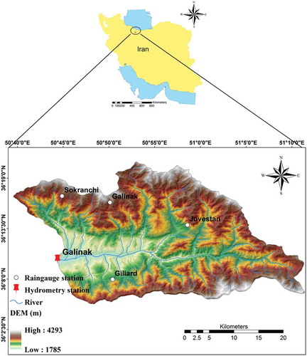
The Taleghan-Rud River, the largest river of the catchment, originates from the Kandovan mountains in the north of Tehran. Recently, flood events have affected the study area, causing significant damage to infrastructure including bridges, rural buildings, main roads, water and gas pipelines and the agricultural sector. For example, in April 2015, a flood event destroyed rural homes and gas pipelines, resulting in an estimated US$86 million in financial losses (Dodangeh et al. 2017). Therefore, developing an accurate streamflow predictive model is necessary for flood control and water resource management and planning in the area.

3 Methodology

3.1 Data collection and preparation

Daily precipitation (P) time series data were assembled from four weather stations equipped with rainfall gauges located within the Taleghan catchment (Fig. 1). The Thiessen polygon approach was used to derive spatially averaged values of P to serve as model input (Melesse et al. 2011). Streamflow (Q) was recorded at the Galinak hydrometric station from 1979 to 2012. In this study, we used $P$ and $Q$ information from past days to predict Q at current time ($Q_t$). Although hydrometeorological (e.g. air temperature and evaporation) and land use change (e.g. the expansion of agricultural areas) variables may also affect the streamflow values, we considered only $P$ and $Q$ variables for two reasons. First, developing an accurate predictive model using limited information is of interest, particularly in regions where data (i.e. meteorological data) are unavailable or defective (i.e. missing value), or the quality of the data is inappropriate. Second, the study area is located in a mountainous region with a mean annual temperature of 9.5°C. So, temperature and its dependent variable (evaporation) might not play a significant role in streamflow prediction. For both P and Q, 70% of each dataset was employed for training (from 1979 to 2002) and 30% (2003–2012) was employed for validation. Although no universal guidelines for dataset division exist, 70:30 is a commonly used ratio for training and validation datasets (Ayele et al. 2017). Since the data were not normally distributed, all input datasets were normalized to enhance the prediction capability of applied models using the following formula:

(1) ${x_i}^{\prime }=\frac{x_i-x_{min}}{x_{max}-x_{min}}$(1)

where

$x_i$ is the i^th untransformed datum of the non-normally distributed data;

${x_i}^{\prime }$ is the i^th transformed datum of the normalized data;

$x_{max}$ is the maximum value of the non-normally distributed data; and

$x_{min}$ is the minimum value of the non-normally distributed data.

3.2 Input/output formulation

In addition to model structure, input combinations have a meaningful effect on the model’s efficiency. Accordingly, the Pearson correlation coefficient (PCC) between individual input variables and the output [present-day Q ($x_{min}$)] served as the criterion in selecting 15 different single or combined input combinations to predict $Q_t$ at the Galinak hydrometric station. Selected combinations of input variables at different lags (n in days – e.g. $P_{t-n}$and $Q_{t-n}$), along with present-day precipitation ($Q_{t-n}$), included:

• seven precipitation-only combinations: $[P_t]-[P_t,P_{t-1}]-[P_t,P_{t-1},P_{t-2}]-[P_t,P_{t-1},P_{t-2},P_{t-3}-[P_t,P_{t-1},P_{t-2},\text{break}{P}_{t-3},P_{t-4}]-[P_t,P_{t-1},P_{t-2},P_{t-3},P_{t-4},P_{t-5}]-[P_t,P_{t-1},\text{break}{P}_{t-2},P_{t-3},P_{t-4},P_{t-5},P_{t-10}]$

• six streamflow-only combinations: $[Q_{t-1}\left]-[Q_{t-1},Q_{t-2}\right]\text{break}-[Q_{t-1},Q_{t-2},Q_{t-3}\left]-[Q_{t-1},Q_{t-2},Q_{t-3},Q_{t-4}]-[Q_{t-1},\text{break}{Q}_{t-2},Q_{t-3},Q_{t-4},Q_{t-5}\right]-[Q_{t-1},Q_{t-2},Q_{t-3},Q_{t-4},Q_{t-5},\text{break}{Q}_{t-10}]$

• two combinations including both precipitation and streamflow. $[Q_{t-1}\left]-[Q_{t-1},Q_{t-2}\right]-[Q_{t-1},Q_{t-2},Q_{t-3}\left]-\text{break}[Q_{t-1},Q_{t-2},Q_{t-3},Q_{t-4}]-[Q_{t-1},Q_{t-2},Q_{t-3},Q_{t-4},\text{break}{Q}_{t-5}\right]-[Q_{t-1},Q_{t-2},Q_{t-3},Q_{t-4},Q_{t-5},Q_{t-10}]$

3.3 Determination of optimal input and operator values

For each of the developed data-mining algorithms, first the best input combinations and then optimal values for different operators (or model parameters) were determined, by trial and error (Kisi et al. 2012, Kisi and Parmar 2016, Khosravi et al. 2018) using the Waikato Environment for Knowledge Analysis (WEKA 3.9) software. For identifying the best input combination, all applied models performed with fixed operator values but different input combinations, and the best combination was determined based on the smallest root mean square error (RMSE) values for the validation/testing dataset. Afterwards, the optimum parameter values of each model were also determined using RMSE values.

3.4 Model development

In the current research, three different kinds of data-mining algorithms, including decision tree algorithms (M5P and RF), a rule algorithm (M5R) and ensemble algorithms (Bagging and Attribute Selected Classifier) were applied for streamflow prediction at the outlet of the Taleghan catchment. Their individual and relative accuracies were determined and compared. Moreover, the statistical time series modelling, the ARIMA model, was also applied to compare the performance of the employed data-mining models.

3.4.1 M5P

The M5P algorithm is an upgraded version of the M5 algorithm introduced by Quinlan (1992), The M5P method can deal with large datasets and is reported to be efficient in handling datasets with missing data. The input space is composed of different subspaces (Fig. 2).

Figure 2. A schematic diagram of the M5P input space and subspaces

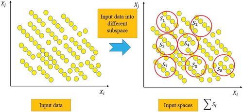
Data from the $\left(X_i,X_j\right)$ space can be categorized into $S_i$ subspaces. Linear regression approaches are then employed to reduce variation, generate several nodes, and create a tree-like structure. The validation of errors to increase the performance of each node is carried out using the standard deviation reduction (SDR; Quinlan 1992):

(2) $SDR={\sigma }_S-\sum _{i=1}^{i=n}\frac{S_i}{\left|S\right|}\cdot {\sigma }_{S_i}$(2)

where

S is the input data received by each node,

$S_i$ is the i^th of n subspaces, and

$\sigma$ is the standard deviation.

After this step, a smoothing process, which integrates all models from the root to the leaf (i.e. all models related to each subspace), is applied to prevent issues of overtraining. At this stage, the final model of the leaf is created. Finally, the results of the leaf data are combined with the linear regression output for that node, and the estimated value,$E^{\prime }$, is passed on to the next higher node (Quinlan 1992, Wang and Witten 1997):

(3) $E^{\prime }=\frac{ne+k_a}{n+k}$(3)

where

a is the predicted/estimated value,

e is the predicted/estimated value passed on to the current node,

$k$ is a constant value, and

n is the number of training/learning steps in the model building.

3.4.2 Random forest (RF)

RF was proposed by Ho (1995) and improved by Breiman (2001). RF is categorized as an ensemble machine learning method. It is composed of multiple trees, where each tree is constructed from bootstrap samples (Breiman et al. 1984). This algorithm is one of the most popular among machine learning algorithms that employ an off-the-shelf procedure to conduct “tree-based learning.” The RF model ranks variables based on their importance in classification or regression problems. In general, this method greatly improves the performance of the model, albeit with some loss of interpretability and a slight increase in bias. Four basic factors must be optimized to obtain the best overall model: the number of trees, the number of features that contain randomly chosen attributes, the maximum depth of the tree, and the number of execution slots. More comprehensive explanations of RF theory are provided by Ho (1995) and Breiman (2001). Figure 3 presents a simple flowchart for the RF model. The model’s architecture is designed to ensure efficient, flexible, and robust classification and regression compared to conventional decision trees.

Figure 3. A simple flowchart describing the RF method (Liaw and Wiener 2002)

3.4.3 M5Rules

M5R is a simple method that generates a set of rule-based algorithms from the M5 model (Ayaz et al. 2015). The M5Rules algorithm (Fig. 4) begins by generating a list of decisions using the separate-and-conquer method. M5Rules works based on replacing the purity heuristic of the decision tree algorithm with a detector that quantifies the reduction in variance. It employs a tree learner on training samples and builds a pruned tree. This process is repeated and next a model tree (i.e. a decision tree with linear models in the leaf) is constructed using the M5 model tree for each repetition, and the best leaf is made a rule. Accordingly, this step transforms the desired leaf into a rule. Further, the tree structure is neglected. In the next step, all samples that have been covered by the rule are removed from the records. When all of the instances are confirmed by one rule, this procedure stops.

Figure 4. The algorithm of M5Rules

This technique is known as a straightforward method for extracting rules from model trees, which benefits from tree learners as an essential part of its structure.

3.4.4 Attribute Selected Classifier (ASC)

Before utilizing a learning algorithm, a vital pre-processing stage must be undertaken to decrease the attribute space and simplify the visualization method. Reducing the amount of data by generating a reduced attribute space eliminates unnecessary features, and minimizes the number of traits. It also ensures that the probability distribution of the datasets differs as much as possible from the first distribution. This classifier considers the weight of the essential subset attributes by evaluating the individual prediction progress of every attribute (Altman 1992). ASC compares each attribute to reach similarity to output. Accordingly, attributes look forward to find the contribution value with the class attribute. This step eliminates attributes to find effective attributes. The elite attributes from the ASC algorithm have been employed in the maximal frequent pattern (MFP) method to reach a considerable reduction with the desired minimum support value. In the attribute selection method, there is a need to select M attributes out of N, complying with the constraint M ≤ N. Attribute selection increases the data quality for the training and testing.

The attribute selection phase contains two main activities: finding an attribute subset and evaluating the subset that is found. Finding an attribute subset is performed using three main algorithms: exponential, random, and sequential algorithms (Boz 2002, Liu and Motoda 2012). Two main approaches can be employed for the validation of the attribute subset: filter and wrapper approaches. Both techniques are independent of finding the attribute subset phase, and they are characterized by their degree of dependence regarding the classification algorithm (Bala et al. 1996). Figure 5 presents a simple flowchart for the ASC algorithm. In the current study, the ASC classifier algorithm is integrated with M5P, RF, and M5R to develop three new hybrid algorithms.

Figure 5. A simple flowchart describing the ASC algorithm modified after (Roject 2009)

3.4.5 Bagging

Bootstrap aggregating or so-called bagging is considered an ensemble meta-algorithm. Through bagging, the model seeks to enhance the prediction power of machine learning algorithms in various regression and classification tasks (see Fig. 6). This algorithm helps to avoid overfitting by reducing the variance of predicted values. Bagging was initially applied to complement decision trees, and it can be combined with any other intelligent computational method. This method is considered to be a particular case of the model averaging approach. In general, for N observations with M features, bootstrapping randomly chooses sample observations. Then the selected sample of observations creates the model in the presence of the subset of features. The best split of the training data helps in choosing the feature from the subset. This cycle continues to make robust models that are trained in parallel. Integrating bagging with a decision tree reduces the overfitting of the training data. This makes the characteristics of sub-models essential factors when combining predictions by bagging.

Figure 6. The Bagging algorithm [b) train a base classifier C_i → b) train a base classifier C_i]

Using the bagging algorithm leads to an improvement of machine learning model stability, e.g. ANNs, regression trees, and classifications (Breiman 1996). In the current study, the integrated bagging classifier algorithm is used with M5P, RF, and M5R to develop three new hybrid algorithms.

3.4.6 Autoregressive integrated moving average (ARIMA)

The ARIMA time series model was introduced by Box and Jenkins (1970). In this model, the univariate time series (i.e. streamflow time series) is considered linear and follows a normal distribution (Box and Jenkins 1970). The main idea is that time series can be decomposed into present values, past values, and random errors. Hence, ARIMA is a combination of auto-regression [AR(p): an additive linear function of p past observations], moving average [MA(q): q random errors], and d, which is an integer that causes a series to be stationary. A general non-seasonal ARIMA model can be written as follows (Box and Jenkins 1970):

(4) ${\mathrm{\Delta }}^{d}y\left(t\right)=c+{\sum }_{j=1}^p{\alpha }_j\times y\left(t-j\right)+\epsilon \left(t\right)+{\sum }_{j=1}^q{\beta }_j\times \epsilon \left(t-j\right)$(4)

where $\mathrm{\Delta }=\left(1-B\right)$, B is the “Backward” operator and $By\left(t\right)=y\left(t-1\right)$, $y\left(t\right)$represents the observation data at time $t$, $t$ is the constant, ${\alpha }_1,\dots ,{\alpha }_p$ are the auto-regressive parameters, $\epsilon \left(t\right)$ is the white noise at time $t$, and ${\beta }_1,\dots ,{\beta }_q$ are the moving average coefficients.

The raw streamflow time series was transformed to be stationary by differencing it d times (i.e. d = 1). The parameters p and q of the ARIMA (p, d, q) structure were estimated by trial and error, and the best parameters were selected when the lowest Akaike information criterion (AIC) value was obtained in the training period (Shibata 1976). Therefore, the ARIMA (2, 1, 1) was applied to train the streamflow prediction model.

3.5 Model validation and comparison

As previously stated, each model was built and trained using the best input combination. Model training employed 70% of the data (training dataset) and led to the determination of optimal values for each operator. Model validation used the remaining 30% of the data (validation dataset). To evaluate each model’s predictive power, some commonly used statistical criteria (Table 1) were applied: RMSE, the coefficient of determination (R²), the bias (BIAS), the mean absolute error (MAE), the Nash-Sutcliffe efficiency (NSE), and the Kling-Gupta efficiency (KGE). Different model validation metrics are required as each has its advantages and disadvantages. R² normalizes for differences between mean and variance of measured and estimated values, but it is sensitive to outliers and should not be used alone for model validation (Legates and McCabe 1999). RMSE shows how differences between measured and predicted data spread out. The main advantage of RMSE and MAE is that they quantify the error in the same unit as for the variables. MAE considers the linear scouring rule and calculates the mean magnitude of the error regardless of direction. NSE is the most widely used metric for measuring and weighing the performance of predictive models. NSE has some advantages, such as: (1) it is not very sensitive to systematic model overestimation or underestimation, (2) it is most widely used and useful in model validation since its dimensional form allows the comparison of performances in different periods and to some extent in different catchments, and (3) it is recommended by the American Society of Civil Engineering, ASCE (1993). However, the main disadvantage of NSE is that squared differences between observed and predicted values are calculated and, hence, large values are more important than low values in this criterion (Legates and McCabe 1999). The main advantage of BIAS is that it shows overestimation/underestimation alongside model performance. KGE uses a decomposition into a correlation term, a bias term, and a variability term and is strongly recommended, particularly in hydrological modelling (Gupta et al. 2009, Kling et al. 2012).

Table 1. Characteristics of performance indicators for the prediction of present-day streamflow ($Q_t$), where $Q_{t_i}^{obs}$ and $Q_{t_i}^{pred}$ are the i^th observed/measured (target) and predicted/estimated (output) values of $Q_{t_i}^{pred}$, respectively; $\overline{Q_t^{pred}}$ is the mean predicted/estimated value of $Q_t,$; N is the number of data points; $\beta$ is the bias ratio ($\beta$); $\gamma$ is the variability ratio ($C{V}_{pred}/C{V}_{obs}$); and CV is the coefficient of variation

Factor	Equation	Ref.
R^2	${\mathrm{R}}^2=1-\hspace{0.17em}\left(\frac{{\sum }_{\mathrm{i}=1}^{\mathrm{i}=\mathrm{N}}{\left(Q_{t_i}^{obs}-Q_{t_i}^{pred}\right)}^2}{{\sum }_{\mathrm{i}=1}^{\mathrm{i}=\mathrm{N}}{\left(Q_{t_i}^{obs}\right)}^2}\right)$	Najafi and Ardabili 2018
RMSE	$\mathrm{R}\mathrm{M}\mathrm{S}\mathrm{E}=\sqrt{\frac{1}{\mathrm{N}}\sum _{\mathrm{i}=1}^{\mathrm{i}=\mathrm{N}}{\left(Q_{t_i}^{pred}-Q_{t_i}^{obs}\right)}^2}$	Najafi and Ardabili 2018
MAE	$\mathrm{M}\mathrm{S}\mathrm{E}=\frac{1}{\mathrm{N}}\sum _{\mathrm{i}=1}^{\mathrm{i}=\mathrm{N}}{\left(Q_{t_i}^{pred}-Q_{t_i}^{obs}\right)}^2$	Najafi and Ardabili 2018
NSE	$\mathrm{N}\mathrm{S}\mathrm{E}=1-\hspace{0.17em}\frac{{\sum }_{\mathrm{i}=1}^{\mathrm{i}=\mathrm{N}}{\left(Q_{t_i}^{pred}-Q_{t_i}^{obs}\right)}^2}{{\sum }_{\mathrm{i}=1}^{\mathrm{N}}{\left(Q_{t_i}^{obs}-\overline{Q_t^{obs}}\right)}^2}$	Moriasi et al. 2007
KGE	$KGE=1-\sqrt{({\left(r-1\right)}^2+{\left(\beta -1\right)}^2+{\left(\gamma -1\right)}^2}$	Gupta et al. 2009, Kling et al. 2012
BIAS	$\mathrm{B}\mathrm{I}\mathrm{A}\mathrm{S}=1-\frac{{\sum }_{\mathrm{i}=1}^{\mathrm{i}=\mathrm{N}}\left(Q_{t_i}^{pred}-Q_{t_i}^{obs}\right)}{{\sum }_{\mathrm{i}=1}^{\mathrm{i}=\mathrm{N}}{Q}_{t_i}^{pred}}$	Legates et al. 1999

Besides statistical criteria, two graphical approaches, namely scatter and box plots, were used to visually compare model performances. A scatter plot can be used to visually estimate the model’s predictive power, where data clustered closest to the 1:1 line (less scattered data points) have the greatest predictive power. The box plot shows the median, quantiles (i.e. first and third), and maximum and minimum predicted values. This approach allows for better judgement regarding which models have the highest accuracy when predicting extreme values.

4 Results and discussion

4.1 Most effective input variables

Analysis of correlations between precipitation and streamflow at different lag times and present-day streamflow ($Q_t$) data (Table 2) showed that streamflow values are clearly more effective in modelling $Q_t$ than precipitation data are. The input $Q_{t-1}$, with a correlation coefficient of 0.96, and inputs $P_{t-3},P_{t-4},\mathrm{a}\mathrm{n}\mathrm{d}{P}_{t-5}$, with correlation coefficients of 0.1, represent, respectively, the inputs with the most and least accurate streamflow predictions. As expected, the larger the lag time, the smaller the correlation coefficient.

Table 2. PCC values between different inputs and output variables

Parameters	PCC
$P_t$	0.19
$P_{t-1}$	0.15
$P_{t-2}$	0.11
$P_{t-3}$	0.10
$P_{t-3}$	0.10
$P_{t-5}$	0.10
$P_{t-10}$	0.11
$Q_{t-1}$	0.96
$Q_{t-2}$	0.93
$Q_{t-3}$	0.91
$Q_{t-3}$	0.90
$Q_{t-5}$	0.89
$Q_{t-10}$	0.82

4.2 Determination of the best input combination

The tested input combinations served to determine the best set of input variables for streamflow modelling (Table 3). The training and validation stage performances of the models (i.e. M5P, RF, M5R, and their hybrid versions using ASC and BA) for different input combinations were assessed based on the RMSE metric. As model inputs, time-lagged streamflows had the highest impact on modelled streamflow ($Q_t$), while precipitation alone had the least effect. Although streamflow cannot be produced without precipitation, and precipitation is the dominant source of streamflow generation in the study area, streamflow cannot be modelled using precipitation alone, especially for large-scale catchments. Therefore, combined inputs of the same-day and lagged precipitation, along with lagged streamflow, should be considered. Several studies showed that applying many input variables does not guarantee a higher predictive power. However, in the current study, for all developed models except ASC, the best input combination (lowest RMSE) was composed of $P_t,P_{t-1},P_{t-2},P_{t-3},P_{t-4},P_{t-5},P_{t-10},Q_{t-1},Q_{t-2},\text{break}{Q}_{t-3},Q_{t-4},Q_{t-5},Q_{t-10}$. For the ASC model, the best combination was $P_t$ and $Q_{t-1}$. While using a combination of all lagged and non-lagged P and Q values, to achieve the best $Q_t$ prediction, does not follow the principle of parsimony, this approach serves to maximize the accuracy of predictions, which was of greater importance in the current study. In most cases, results showed that antecedent Q has the largest impact on streamflow prediction (Yaseen et al. 2015, 2016). As Q is a product of precipitation, considering both antecedent precipitation and discharge may enhance the results. Testing the various input combinations can be considered a sensitivity analysis, where an input variable is removed from the modelling process each time and the RMSE is calculated. Differences in RMSE can indicate the impact of the removed variable. Based on this procedure, $Q_{t-1}$ had the highest impact on the M5P- and M5R-predicted streamflow.

Table 3. Best model input combinations during the training and validation phases based on the RMSE (m³ s⁻¹). ALLPQ = $P_t,P_{t-1},P_{t-2},P_{t-3},P_{t-4},P_{t-5},P_{t-10},Q_{t-1},\text{break}{Q}_{t-2},Q_{t-3},Q_{t-4},Q_{t-5},Q_{t-10}$

Model Inputs	Model validation phase RMSE (m^3 s^−1)
	M5P		RF		M5R		ASC		Bagging
	TRAIN.	VALID.	TRAIN.	VALID.	TRAIN.	VALID.	TRAIN.	VALID.	TRAIN.	VALID.
$P_t,P_{t-1},P_{t-2},P_{t-3},P_{t-4},P_{t-5},P_{t-10},Q_{t-1},Q_{t-2},Q_{t-3},Q_{t-4},Q_{t-5},Q_{t-10}$	14.0	14.7	13.8	14.9	14.0	14.7	14.0	14.7	13.9	14.7
$P_t,P_{t-1}$	13.9	14.7	12.9	15	13.9	14.7	13.9	14.7	13.5	14.7
$P_t,P_{t-1},P_{t-2}$	13.9	14.6	12.1	14.9	13.9	14.6	13.9	14.6	13.3	14.7
$P_t,P_{t-1},P_{t-2},P_{t-3}$	13.8	14.6	11.4	15.1	13.8	14.6	13.9	14.6	13.1	14.7
$P_t,P_{t-1},P_{t-2},P_{t-3}$	13.8	14.6	10.7	15.1	13.8	14.6	13.8	14.6	13.0	14.7
$P_t,P_{t-1},P_{t-2},P_{t-3},P_{t-4},P_{t-5}$	13.8	14.5	10.0	15.0	13.8	14.5	13.8	14.5	12.8	14.7
$P_t,P_{t-1},P_{t-2},P_{t-3},P_{t-4},P_{t-5},P_{t-10}$	13.7	14.5	9.3	15.0	13.7	14.5	13.7	14.5	12.6	14.6
$Q_{t-1}$	3.7	4.3	2.4	4.7	3.7	4.3	3.7	4.3	3.4	4.4
$Q_{t-1},Q_{t-2}$	3.5	4.4	1.6	4.5	3.6	4.4	3.7	4.3	3.3	4.3
$Q_{t-1},Q_{t-2},Q_{t-3}$	3.6	4.4	1.5	4.5	3.7	4.4	3.7	4.3	3.1	4.3
$Q_{t-1},Q_{t-2},Q_{t-3}$	3.6	4.4	1.4	4.5	3.5	4.5	3.7	4.3	4.3	4.2
$$Q_{t-1},Q_{t-2},Q_{t-3},Q_{t-4},Q_{t-5}$$	3.6	4.4	1.4	4.4	3.6	4.5	3.7	4.3	4.2	4.2
$Q_{t-1},Q_{t-2},Q_{t-3},Q_{t-4},Q_{t-5},Q_{t-10}$	3.7	4.4	1.4	4.4	3.6	4.4	3.6	4.2	3.1	4.4
$P_t,Q_{t-1}$	3.3	4.2	1.7	4.4	3.2	4.3	3.3	4.2	3.0	4.1
$\mathrm{A}\mathrm{l}\mathrm{l}\mathrm{P}\mathrm{a}\mathrm{n}\mathrm{d}\mathrm{Q}$	3.3	3.9	1.2	4.0	3.3	3.9	3.2	4.3	2.7	4.0

Generally, the type of precipitation and its distribution in terms of skewness can have a strong effect on the accuracy of streamflow prediction (Kisi and Parmar 2016). Since the precipitation dataset shows skewness in the present study (whole dataset = 1.25, training dataset = 1.15, and testing dataset = 1.31), precipitation alone does not have the ability to predict streamflow accurately. Another factor that affects the hydrological behaviour of the catchment is that a small part of the precipitation at high altitudes occurs in the form of snow, which results in a different rainfall-runoff response.

The results showed that the streamflow generation needs some time for concentration; hence, considering precipitation with lag time ($Q_{t-1}$, $P_{t-2}$ and so on) is much more effective than considering precipitation without any lag time (P). Our result is in accordance with Adnan et al. (2019), who stated that with only precipitation data, streamflow cannot be predicted with good accuracy. The results also revealed that generally, streamflow with a lag time ($Q_{t-1},Q_{t-2}$ and so on) is much more effective than precipitation with a lag time ($P_{t-1}$, $P_{t-2}$and so on) for streamflow prediction. When using only the streamflow with 1 d lag time, we can achieve good results for streamflow prediction (Table 3, combination no. 8).

4.3 Model validation

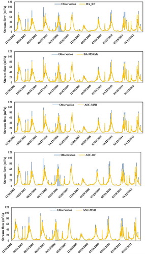
For the validation period, the time series plot of observed and model-predicted streamflow values (Fig. 7) suggests that although all applied algorithms have a high prediction power in overall streamflow prediction, BA-RF and ASC-RF was not able to predict peak values accurately. As hydrographs were unable to capture all aspects of model performance, additional model validation criteria were implemented. Given identical input combinations, differences in model prediction power and accuracy can be linked to differences in model structure and complexity.

Figure 7. Validation period streamflow: blue = observed/measured; orange = model-predicted/estimated

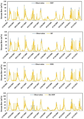
Figure 7. (Continued)

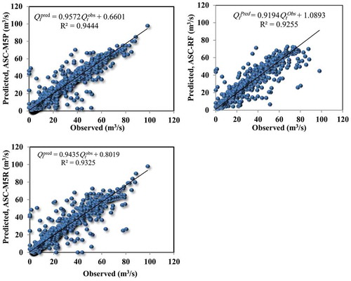
Scatter plots of observed vs. model-predicted streamflow for the validation phase (Fig. 8) show that the BA-M5P model with an R² of 0.95 and a fitted linear regression equation $Q_t^{pred}=0.96Q_t^{pred}+0.61$ and the ASC-M5P model with an R² of 0.94 and a fitted linear regression equation $Q_t^{pred}=0.96Q_t^{pred}+0.61$ have less scattered estimates than other models, indicating predicted values closer to the observed values. The standalone model with almost identical R² values shows the most scattered estimated streamflow values, i.e. further from observed values compared to the BA- and ASC-based models.

Figure 8. Scatter plots of model-predicted/estimated vs. observed/measured streamflow values ($Q_t^{\mathrm{p}\mathrm{r}\mathrm{e}\mathrm{d}}$ and $Q_t^{\mathrm{p}\mathrm{r}\mathrm{e}\mathrm{d}}$, respectively) in the validation period

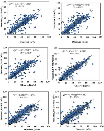
Figure 8. (Continued)

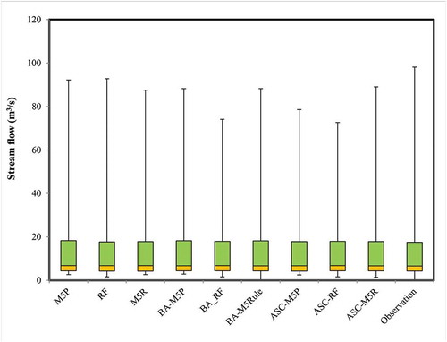
Values of $Q_t^{\mathrm{o}\mathrm{b}\mathrm{s}}$ and $Q_t^{\mathrm{p}\mathrm{r}\mathrm{e}\mathrm{d}}$(for each model) plotted as a box plot (Fig. 9) show the median (Q₅₀), first quartile (Q₂₅), and third quartile (Q₇₅) of $Q_t^{\mathrm{p}\mathrm{r}\mathrm{e}\mathrm{d}}$values to be similar to those of the $Q_t^{\mathrm{o}\mathrm{b}\mathrm{s}}$ values. The main difference between the model predictions and observed data was in the data range (minimum and maximum values), as all applied models were incapable of correctly predicting extreme observed $$Qt$$ values.

Figure 9. Box plot of observed/measured and predicted/estimated streamflow values for the validation period

Statistical performance indices for model predictive power evaluation in the validation period are presented in Table 4. AI and physically based models have a very good performance when NSE > 0.75, according to the model performance classification recommended by Moriasi et al. (2007). In this study, the BA-M5P model, with an RMSE of 3.23 m³ s⁻¹, MAE of 1.34 m³ s⁻¹, NSE of 0.933 and KGE of 0.954, gave the best performance. Also, all developed algorithms have a higher prediction capability than physically based models (i.e. section 4.4).

Table 4. Comparison of the model performance using statistical criteria

Model	R^2	RMSE (m^3 s^−1)	MAE (m^3 s^−1)	NSE	KGE	BIAS
M5P	0.917	4.32	1.45	0.904	0.927	−0.26
RF	0.915	4.40	1.56	0.901	0.924	−0.18
M5R	0.917	4.36	1.48	0.900	0.921	−0.07
BA-M5P	0.954	3.23	1.34	0.933	0.954	−0.70
BA-RF	0.927	4.00	1.42	0.925	0.943	0.15
BA-M5R	0.937	3.77	1.42	0.917	0.953	−0.11
ASC-M5P	0.944	3.80	1.39	0.931	0.950	0.33
ASC-RF	0.925	4.11	1.42	0.914	0.952	0.22
ASC-M5R	0.932	3.91	1.38	0.916	0.948	0.43
ARIMA	0.883	5.16	1.93	0.868	0.913	−0.34
Dodangeh et al. 2018 (IHACRES)	Not reported	Not reported	Not reported	0.75	Not reported	Not reported
Dodangeh et al. 2019 (HSPF)	0.83	Not reported	Not reported	Not reported	Not reported	Not reported
Noor et al. 2014 (SWAT)	0.82	Not reported	Not reported	0.80	Not reported	Not reported

Overall, M5P (RMSE = 4.32 m³ s⁻¹, MAE = 1.45 m³ s⁻¹, NSE = 0.904, KGE = 0.927 and BIAS = −0.263) outperformed the other standalone models in terms of predictive power. Although M5P had difficulty predicting extremely high flows, this model was found to predict extremely low and average streamflows much better than the other models applied. Results show that the performance of the hybrid algorithms depends on the base algorithm. Generally, the BA-based models outperform the ASC-based models. This may be due to the fact that the bagging model combines multiple weak learners, which leads to a stronger learner than the ASC model. Therefore, it often outperforms the single weak learners, such as M5P, or other models applied.

The BA-M5R model, followed by the ASC-RF, ASC-M5P, ASC-M5R, BA-M5R, M5P, RF and M5R (in that order), had the highest predictive power after BA-M5P according to KGE and was most accurate in its predictions. The main benefit of the M5P model is that it has the ability to efficiently handle many datasets with many attributes and dimensions. As the minimization of the standard deviation in the intra-subset class values is used as the splitting criterion for the M5P model in contrast to other decision tree algorithms, in which maximization of information gain is the splitting criterion (Hashmi et al. 2015), this model can predict the streamflow with high accuracy.

The calculated BIAS values for the developed models, except for BA-RF, ASC-M5P, ASC-RF and ASC-M5R, were negative, indicating an overestimation of streamflow values using these algorithms.

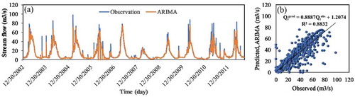
The ability of the developed data-mining models over the statistical time series modelling, the ARIMA model, was also compared to predict streamflow. The results of the ARIMA model for the validation period are given in Table 4. The ARIMA model achieved the lowest accuracy (R² = 0.883, NSE = 0.868, KGE = 0.913) and highest error (RMSE = 5.16 m³ s⁻¹ and MAE = 1.93 m³ s⁻¹), not only compared to the standalone M5P, RF and M5R but also compared to their hybrid counterparts. The time series plot of the observed and ARIMA-predicted streamflow (Fig. 10(a)) shows that the ARIMA model cannot predict the peak values of the streamflow. The scatter plot of observed vs. ARIMA-predicted streamflow for the validation phase (Fig. 10(b)) shows that the predicted streamflow through the stochastic ARIMA model is most scattered than the observed values. Therefore, it can be concluded that the developed nonlinear data-mining models are more capable of predicting the streamflow values compared to the stochastic time series models. Moreover, the results of the ARIMA model confirm that rainfall is an important variable in predicting streamflow and that accurate $Q_t$ prediction using only the lag times of the streamflow is impossible.

Figure 10. (a) Time series and (b) scatter plots of the observed and ARIMA-predicted streamflow (m³ s⁻¹)

4.4 Comparison with the literature

Dodangeh et al. (2018, 2019) predicted the streamflow of the Taleghan catchment using the lumped model IHACRES and the HSPF model with the same data as in the present study. Comparing their results with ours shows that the data-mining algorithms examined here have higher predictive power than the conceptual-based models IHACRES (NSE = 0.75; present study NSE = 0.95) and HSPF (R² = 0.83; present study R² = 0.954). The lower performance of the latter is due to the fact that snowfall and snowmelt runoff were not considered in their studies, while data-mining algorithms could find the best model based on the inputs and output and implicitly taking snowfall and melt processes into account.

Noor et al. (2014) implemented the SWAT model in the same study area and reported that the SWAT model (with R² = 0.82 and NSE = 0.80) gave a reasonable performance and, overall, underestimated streamflow values. They reported that based on the literature, the SWAT model underestimates streamflow in mountainous catchments where snowmelt plays a key role in streamflow generation. This happens due to the simple temperature-index method in snowpack and snowmelt modelling that is used in the SWAT model (Akhavan et al. 2010, Pradhanang et al. 2011). The simultaneous occurrence of snowmelt and spring rainfall in a mountainous catchment like Taleghan can cause a high maximum discharge, and hence, to achieve the best performance through physically based models, these hydrological processes must be considered (directly or indirectly) in the modelling process.

Also, the Taleghan catchment is located in a semi-arid region of Iran and therefore, has a relatively fast hydrologic response to precipitation occurrences. Models with a linear structure like IHACRES cannot provide accurate predictions for this type of catchment, particularly predictions of high discharges, while AI algorithms due to their non-linear structure have a higher prediction capability, thus, application of physically based models for streamflow prediction, particularly during winter for mountainous catchments similar to Taleghan, is not recommended when snow characteristics and runoff from snow melting are not included in the model.

Previous researchers have modelled streamflow using AI, and their results can be compared to those of the current study. Kisi et al. (2013) modelled streamflow in Turkey using gene expression programming (GEP), ANFIS, ANN, and multiple linear regression models and the results were very good to reasonable, with R² values of 0.97, 0.93, 0.80 and 0.70, respectively. Modelling daily flows in two large catchments and five smaller catchments in India, Rajurak et al. (2004) compared operational ANN hydrological models previously used in India by the World Meteorological Organization and found the best model achieved an R² of 0.92 and an NSE of 0.70. Also, their results showed that Q with lag time enhanced the models’ predictive power. Rezaie-Balf et al. (2017) employed ANNs, a model tree algorithm, and multivariate adaptive regression splines to predict streamflow in northern Iran’s Tajan catchment using rainfall, discharge, evaporation, morning relative humidity, noon relative humidity, evening relative humidity, wind velocity, maximum temperature, and minimum temperature, with and without lag time as input. The study focused on the effects of input size, the number of effective input variables for the streamflow prediction as well as the length of data time-series on the quality of streamflow simulations by the applied algorithms. They found that data-mining algorithms outperformed the ANN and Multivariate adaptive regression spline (MARS) models. Similarly, the data-mining approaches developed in the current research (Table 4) were satisfactory to highly successful in predicting streamflow values (0.90 < NSE < 0.93). Also, Rezaie-Balf et al. (2017) found that the best input variables are a combination of rainfall and discharge variables, which is also confirmed in the current study.

Models differ in terms of complexity and structure, and, consequently, each model has distinct advantages and disadvantages for a given context. A wide range of data intelligence, data mining, and physically based models have been implemented in many studies on simulating hydrological variables such as streamflow. In many cases, these models were found to exhibit a high predictive power for streamflow. Ultimately, it is recommended that streamflow be predicted using a variety of strong physically based models (e.g. SWAT, Wetspa, Hydrologic Engineering Center-Hydrologic Modeling System (HEC-HMS)), and that their outputs are compared to those of the proposed data-mining algorithms. Based on the model complexity, data requirements, and accuracy, an optimal model can be recommended for the given context.

There are several limitations inherent in predicting hydrological times series with AI models. For each model, optimal input combinations and optimal values for each operator apply only to the present catchment. To model other catchments, all modelling steps must be performed again, from start to finish. Another limitation is that AI models cannot predict streamflow with high accuracy using precipitation, evaporation, or soil information, unless antecedent streamflow is also used as an input to the model. This phenomenon is primarily due to weak relationships between streamflow as dependent data, and precipitation, evaporation, and soil as independent data (Tongal and Booij 2018). For future research, we recommend investigating the efficiency of the developed models in other catchments with different hydro-meteorological conditions. We also recommend investigating the capability of the models with input variables from neighbouring hydrometric stations in the catchment.

5 Conclusions

Given the complex and nonlinear nature of streamflow, modelling streamflow has remained a challenge for hydrologists. Although there are no universal guidelines for streamflow predictions, to date many algorithms have been developed and used for this purpose. In the present study, several new standalone and hybrid data-mining algorithms were implemented for streamflow prediction in Iran’s Taleghan catchment. The main findings can be summarized as follows:

• Streamflow for preceding days is more effective in predicting current streamflow than precipitation is.

• Due to the different structures of the AI models, the best input combinations are not the same for all applied models.

• The BA-M5P model outperformed the other models in terms of accuracy. It was followed by (in descending order) ASC-RF, ASC-M5P, ASC-M5R, BA-M5R, M5P, RF, M5R, and ARIMA.

• The BIAS values show that the BA-RF, ASC-M5P, ASC-RF and ASC-M5R algorithms overestimated streamflow and the other models underestimated streamflow.

• According to the box plots, none of the applied models have the ability to predict extreme flow values.

• Hybrid algorithms can enhance the predictive power of standalone models.

• AI algorithms gave a higher performance than the physically based models IHACRES, SWAT and HSPF for the Taleghan catchment.

The findings of the current study have practical value for water resource managers, hydrologists, the Iranian Water Resources Management Bureau, and other decision-makers for present-day and future flood management.

Software availability

Waikato Environment for Knowledge Analysis (WEKA) is an open-source software program written in Java and developed at the University of Waikato, New Zealand. It is free software licensed under the GNU General Public License. Software and documentation (user manual and training material) are freely available at https://www.cs.waikato.ac.nz/ml/weka/downloading.html.

Disclosure statement

No potential conflict of interest was reported by the authors.

Data availability statement

The data that support the findings of this study are available from the corresponding author upon reasonable request.

Additional information

Funding

This research project was supported by Ferdowsi University of Mashhad, Mashhad, Iran.

References

- Adnan, M., et al., 2019. Least square support vector machine and multivariate adaptive regression splines for streamflow prediction in mountainous basin using hydro-meteorological data as inputs. Journal of Hydrology. (in press). doi:10.1016/j.jhydrol.2019.124371.
- Akhavan, S., et al., 2010. Application of swat model to investigate nitrate leaching in hamadan–bahar watershed, Iran. Agriculture, Ecosystems & Environment, 139 (4), 675–688. doi:10.1016/j.agee.2010.10.015.
- Altman, N.S., 1992. An introduction to kernel and nearest-neighbor nonparametric regression. The American Statistician, 46, 175–185.
- ASCE. 1993. Criteria for evaluating watershed models. Journal of Irrigation and Drainage Engineering, 119 (3), 429–442.
- Auria, L. and Moro, R.A., 2009. Support Vector Machines (SVM) as a technique for solvency analysis. DIW Berlin Discussion Paper No. 811. Available at SSRN: doi:10.2139/ssrn.1424949.
- Ayaz, Y., Kocamaz, A.F., and Karakoç, M.B., 2015. Modeling of compressive strength and UPV of high-volume mineral-admixtured concrete using rule-based M5 rule and tree model M5P classifiers. Construction and Building Materials, 94, 235–240. doi:10.1016/j.conbuildmat.2015.06.029.
- Ayele, G., et al., 2017. Streamflow and sediment yield prediction for watershed prioritization in the Upper Blue Nile River Basin. Ethiopia Water, 9, 782.
- Baez-Villanueva, O.M., et al., 2020. RF-MEP: a novel Random Forest method for merging gridded precipitation products and ground-based measurements. Remote Sensing of Environment, 239, 111606. doi:10.1016/j.rse.2019.111606.
- Bahat, Y., et al., 2009. Rainfall-runoff modelling in a small hyper-arid catchment. Journal of Hydrology, 373 (1–2), 204–217. doi:10.1016/j.jhydrol.2009.04.026.
- Bala, J., et al. 1996. Using learning to facilitate the evolution of features for recognizing visual concepts. Evolutionary Computation, 4 (3), 297–311. doi:10.1162/evco.1996.4.3.297.
- Beven, K.J., 2001. Rainfall-runoff modelling: the primer. 2nd ed. Chichester, England: John Wiley, Sons, 449 p. ISBN: 978-0-470-71459-1.
- Beven, K.J., 2005. Rainfall-runoff modelling: introduction. Encyclopedia of Hydrological Sciences. doi:10.1002/0470848944.
- Bhuiyan, M.A., Nikolopoulos, E.I., and Anagnostou, E.N., 2019. Machine learning-based blending of satellite and reanalysis precipitation datasets: a multiregional tropical complex terrain evaluation. Journal of Hydrometeorology, 20 (11), 2147–2161. doi:10.1175/JHM-D-19-0073.1.
- Box, G.E.P. and Jenkins, G.M., 1970. Time series analysis, forecasting, and control. Francisco Holden-Day (6), 712. ISBN: 978-1-118-67502-1.
- Boz, O., 2002. Feature subset selection by using sorted feature relevance. in ICMLA. In Proc. Intl. Conf. on Machine Learning and Applications.Published in ICMLA 2002. Citeseer.
- Breiman, L., et al., 1984. Classifcation and regression trees. Belmont, CA: Wadsworth International Group, 432.
- Breiman, L., 1996. Bagging predictors. Machine Learning, 24 (2), 123–140. doi:10.1007/BF00058655.
- Breiman, L., 2001. Random forests. Machine Learning, 45 (1), 5–32. doi:10.1023/A:1010933404324.
- Bui, D., et al. 2018a. New hybrids of anfis with several optimization algorithms for flood susceptibility modeling. Water, 10 (9), 1210. doi:10.3390/w10091210.
- Bui, D., et al. 2018b. Novel hybrid evolutionary algorithms for spatial prediction of floods. Scientific Reports, 8 (1), 15364. doi:10.1038/s41598-018-33755-7.
- Burges, C.J. 1998. A tutorial on support vector machines for pattern recognition. Data Mining and Knowledge Discovery, 2, 121–167. doi:10.1023/A:1009715923555.
- Çelik, Ö., Teke, A., and Yildirim, H.B., 2016. The optimized artificial neural network model with Levenberg–Marquardt algorithm for global solar radiation estimation in Eastern Mediterranean Region of Turkey. Journal of Clean Production, 116, 1–12. doi:10.1016/j.jclepro.2015.12.082.
- Chang, T.K., et al., 2017. Choice of rainfall inputs for event-based rainfall-runoff modelling in a catchment with multiple rainfall stations using data-driven techniques. Journal of Hydrology, 545, 100–108. doi:10.1016/j.jhydrol.2016.12.024.
- Chen, W., et al., 2019. Spatial prediction of groundwater potentiality using ANFIS ensembled with Teaching-learning-based and Biogeography-based optimization. Journal of Hydrology, 527, 435–448. doi:10.1016/j.jhydrol.2019.03.013.
- Clark, M.P., et al., 2017. The evolution of process-based hydrologic models: historical challenges and the collective quest for physical realism. Hydrology and Earth System Sciences, 21 (7), 3427–3440. doi:10.5194/hess-21-3427-2017.
- Contreras, J., et al., 2018. Rainfall monitoring network design using conditioned Latin hypercube sampling and satellite precipitation estimates: an application in the ungauged Ecuadorian Amazon. International Journal of Climatology, 39 (4), 2209–2226. doi:10.1002/joc.5946.
- Danandeh Mehr, A., et al., 2019. A hybrid support vector regression–firefly model for monthly rainfall forecasting. International Journal of Environmental Science and Technology, 16 (1), 335–346. doi:10.1007/s13762-018-1674-2.
- Dawson, C.W. and Wilby, R., 1998. An artificial neural network approach to rainfall-runoff modelling. Hydrological Sciences Journal, 43 (1), 47–66. doi:10.1080/02626669809492102.
- Dehghani, M., Riahi-Madvar, H., Hooshyaripor, F., Mosavi, A., Shamshirband, S., Zavadskas, E.K., and Chau, K. 2019. Prediction of hydropower generation using grey wolf optimization adaptive neuro-fuzzy inference system. Energies, 12 (2), Article no. 289. doi:10.3390/en12020289.
- Demirel, M.C., Booij, M.J., and Hoekstra, A.Y., 2015. The skill of seasonal ensemble low-flow forecasts in the Moselle River for three different hydrological models. Hydrology and Earth System Sciences, 19 (1), 275–291. doi:10.5194/hess-19-275-2015.
- Dodangeh, E., et al., 2019. Joint frequency analysis and uncertainty estimation of coupled rainfall–runoff series relying on historical and simulated data. Hydrological Sciences Journal. (In press). doi:10.1080/02626667.2019.1704762.
- Dodangeh, E., Shahedi, K., Solaimani, K., and Kossieris, P., 2017. Usability of BLRP model for hydrological applications in arid and semi arid regions with limited precipitation data. Modeling Earth Systems and Environment, 3 (2), 539–555.
- Dodangeh, E., Shahedi, K., and Solaimani, 2018. Application of Copula theory for IHACRES hydrologic model evaluation (Case study: Taleghan watershed). Journal of Earth and Space Physics, 44 (1), 71–88. (in Persian).
- Furundzic, D., 1998. Application example of neural networks for time series analysis: rainfall–runoff modelling. Signal Processing, 64 (3), 383–396. doi:10.1016/S0165-1684(97)00203-X.
- Gautam, M.R., Atanabe, K.W., and Aegusa, H.S., 2000. Runoff analysis in humid forest catchment with artificial neural network. Journal of Hydrology, 235 (1–2), 117–136. doi:10.1016/S0022-1694(00)00268-7.
- Gupta, H.V., et al., 2009. Decomposition of the mean squared error and NSE performance criteria: implications for improving hydrological modelling. Journal of Hydrology, 377 (1–2), 80–91. doi:10.1016/j.jhydrol.2009.08.003.
- Habib, E., et al., 2014. Effect of bias correction of satellite-rainfall estimates on runoff simulations at the source of the Upper Blue Nile. Remote Sensing, 6 (7), 6688–6708. doi:10.3390/rs6076688.
- Hashmi, S., Halawani, S.M., Barukab, O.M., and Ahmad, A. 2015. Model trees and sequential minimal optimization based support vector machine models for estimating minimum surface roughness value. Applied Mathematical Modelling, 39 (3–4), 1119–1136.
- He, Y., Bárdossy, A., and Zehe, E., 2011. A review of regionalisation for continuous streamflow simulation. Hydrology and Earth System Sciences, 15 (11), 3539–3553. doi:10.5194/hess-15-3539-2011.
- Hengl, T., et al., 2017. Soil grids 250 m: global gridded soil information based on machine learning. PLoS One, 12 (2), e0169748. doi:10.1371/journal.pone.0169748.
- Herrnegger, M., Senone, T., and Nachtnebel, H.P., 2018. Adjustment of spatio-temporal precipitation patterns in a high Alpine environment. Journal of Hydrology, 556, 913–921. doi:10.1016/j.jhydrol.2016.04.068.
- Ho, T.K., 1995. Random decision forests. In: Document analysis and recognition, 1995, proceedings of the third international conference on document analysis and recognition (Volume 1). IEEE, 278–282.
- Honorato, A.G., Silva, G.B., and Santos, C.A. 2018. Monthly streamflow forecasting using neuro-wavelet techniques and input analysis. Hydrological Science Journal, 63 (15–16), 2060–2075.
- Hsu, K.I., Gupta, H.V., and Sorooshian, S., 1995. Artificial neural network modelling of the rainfall‐runoff process. Water Resources Research, 31 (10), 2517–2530. doi:10.1029/95WR01955.
- Jeong, D. and Kim, Y.O., 2005. Rainfall‐runoff models using artificial neural networks for ensemble stream flow prediction. Hydrological Process, 19 (19), 3819–3835. doi:10.1002/hyp.5983.
- Khosravi, K., et al., 2019b. Stochastic modeling of groundwater fluoride contamination: introducing lazy learners. Groundwater. (in press). doi:10.1111/gwat.12963.
- Khosravi, K., et al., 2019a. Meteorological data mining and hybrid data-intelligence models for reference evaporation simulation: a case study in Iraq. Computers and Electronics in Agriculture, 167, 105041. doi:10.1016/j.compag.2019.105041.
- Khosravi, K., et al., 2018. Quantifying hourly suspended sediment load using data mining models: case study of a glacierized Andean catchment in Chile. Journal of Hydrology, 567, 165–179. doi:10.1016/j.jhydrol.2018.10.015.
- Kirchner, J.W., 2006. Getting the right answers for the right reasons: linking measurements, analyses, and models to advance the science of hydrology. Water Resources Research, 42 (3). doi:10.1029/2005WR004362.
- Kisi, O. and Parmar, K.S., 2016. Application of least square support vector machine and multivariate adaptive regression spline models in long term prediction of river water pollution. Journal of Hydrology, 534, 104–112. doi:10.1016/j.jhydrol.2015.12.014.
- Kisi, O., Shiri, J., and Tombul, M., 2012. Modelling rainfall-runoff process using soft computing techniques. Computers & Geosciences, 51, 108–117. doi:10.1016/j.cageo.2012.07.001.
- Kisi, O., Shiri, J., and Tombul, M., 2013. Modeling rainfall-runoff process using soft computing techniques. Computer and Geoscience, 51, 108–117. doi:10.1016/j.cageo.2012.07.001.
- Kling, H., Fuchs, M., and Paulin, P., 2012. Runoff conditions in the upper Danube basin under an ensemble of climate change scenarios. Journal of Hydrology, 424-425, 264–277. doi:10.1016/j.jhydrol.2012.01.011.
- Kundzewicz, Z.W., et al., 2014. Flood risk and climate change: global and regional perspectives. Hydrological Sciences Journal, 59 (1), 1–28. doi:10.1080/02626667.2013.857411.
- Legates, D.R. and McCabe, G.J., 1999. Evaluating the use of “goodness-of-fit” measures in hydrologic and hydroclimatic model validation. Water Resources Research, 35 (1), 233–241. doi:10.1029/1998WR900018.
- Liaw, A., and Wiwnwe, M. 2002. Classification and Regression by random Forest. R News. http://cogns.northwestern.edu/cbmg/LiawAndWiener2002.pdf.
- Liu, H. and Motoda, H., 2012. Feature selection for knowledge discovery and data mining. Vol. 454. Springer Science & Business Media.
- Lohani, A.K., Goel, N.K., and Bhatia, K.K.S., 2010. Comparative study of neural network, fuzzy logic and linear transfer function techniques in daily rainfall‐runoff modelling under different input domains. Hydrological Process, 25 (2), 175–193. doi:10.1002/hyp.7831.
- Long, H., Zhang, Z., and Su, Y., 2014. Analysis of daily solar power prediction with data-driven approaches. Applied Energy, 126, 29–37. doi:10.1016/j.apenergy.2014.03.084.
- Mallikarjuna, P., Suresh Babu, C.H., and Reddy, A.J.M., 2009. Rainfall—runoff modelling using artificial neural networks. ISH Journal of Hydraulic Engineering, 15 (1), 24–33. doi:10.1080/09715010.2009.10514928.
- Mehdizadeh, S., et al., 2020. Drought modeling using classic time series and hybrid wavelet-gene expression programming models. Journal of Hydrology, 587, 125017. doi:10.1016/j.jhydrol.2020.125017.
- Melesse, A., et al., 2011. Suspended sediment load prediction of river systems: an artificial neural network approach. Agricultural Water Management, 98 (5), 855–866. doi:10.1016/j.agwat.2010.12.012.
- Mellit, A., et al., 2010. An adaptive model for predicting of global, direct and diffuse hourly solar irradiance. Energy Conversion and Management, 51 (4), 771–782. doi:10.1016/j.enconman.2009.10.034.
- Minns, A.W. and Hall, M.J., 1996. Artificial neural networks as rainfall-runoff models. Hydrological Sciences Journal, 41 (3), 399–417. doi:10.1080/02626669609491511.
- Mishra, S., et al., 2018. Rainfall-runoff modeling using clustering and regression analysis for the river brahmaputra basin. Journal of the Geological Society of India, 92 (3), 305–312. doi:10.1007/s12594-018-1012-9.
- Moriasi, D., et al., 2007. Model evaluation guidelines for systematic quantification of accuracy in watershed simulations. Transactions of the ASABE, 50 (3), 885–900. doi:10.13031/2013.23153.
- Najafi, B. and Ardabili, S.F., 2018. Application of ANFIS, ANN, and logistic methods in estimating biogas production from spent mushroom compost (SMC). Resources, Conservation and Recycling, 133, 169–178. doi:10.1016/j.resconrec.2018.02.025.
- Nayak, P.C., et al., 2004. A neuro-fuzzy computing technique for modelling hydrological time series. Journal of Hydrology, 291 (1–2), 52–66. doi:10.1016/j.jhydrol.2003.12.010.
- Noor, H., et al., 2014. Comparison of single-site and multi-site based calibrations of SWAT in Taleghan Watershed, Iran. International Journal of Engineering, 27 (11), 1645–1652.
- Nourani, V., 2017. An Emotional ANN (EANN) approach to modelling rainfall-runoff process. Journal of Hydrology, 544, 267–277. doi:10.1016/j.jhydrol.2016.11.033.
- Nourani, V., Kisi, Ö., and Komasi, M., 2011. Two hybrid Artificial Intelligence approaches for modelling rainfall-runoff process. Journal of Hydrology, 402 (1–2), 41–59. doi:10.1016/j.jhydrol.2011.03.002.
- Nourani, V., Komasi, M., and Mano, A., 2009. A multivariate ANN-wavelet approach for rainfall-runoff modelling. Water Resources Management, 23 (14), 2877–2894. doi:10.1007/s11269-009-9414-5.
- Olaiya, F. and Adeyemo, A.B., 2012. Application of data mining techniques in weather prediction and climate change studies. International Journal of Information Engineering and Electronic Business, 4 (1), 51–59. doi:10.5815/ijieeb.2012.01.07.
- Ömer Faruk, D., 2010. A hybrid neural network and ARIMA model for water quality time series prediction. Engineering Applications of Artificial Intelligence, 23 (4), 586–594. doi:10.1016/j.engappai.2009.09.015.
- Pradhanang, S.M., et al., 2011. Application of swat model to assess snowpack development and streamflow in the cannonsville watershed, new york, USA. Hydrological Processes, 25 (21), 31268–33277. doi:10.1002/hyp.8171.
- Quinlan, J.R., 1992. Learning with continuous classes. In: 5th Australian joint conference on artificial intelligence. Samaniego: World Scientific, 343–348.
- Rajurak, M.P., Kothyari, U.C., and Chaube, U.C., 2004. Modeling of the daily rainfall-runoff relationship with artificial neural network. Journal of Hydrology, 285 (1–4), 96–113. doi:10.1016/j.jhydrol.2003.08.011.
- Rezaie-Balf, M., Zahmatkesh, Z., and Kim, S., 2017. Soft computing techniques for rainfall-runoff simulation: local non–parametric paradigm vs. model classification methods. Water Resource Management, 31 (12), 3843–3865. doi:10.1007/s11269-017-1711-9.
- Rogers, W.F., 1972. new concept in hydrograph analysis. Water Resources Research, 8 (4), 937–981. doi:10.1029/WR008i004p00973.
- Rojek, I., 2009. Classifier models in intelligent CAPP systems. In Man-machine interactions (pp. 311–319). Berlin, Heidelberg: Springer. Engineering, 119 (3), 429–442.
- Salih, S., et al., 2019. River suspended sediment load prediction based on river discharge information: application of newly developed data mining models. Hydrological Sciences Journal. (In press). doi:10.1080/02626667.2019.1703186.
- Shibata, R., 1976. Selection of the order of an autoregressive model by Akaike’s information criterion. Biometrika, 63 (1), 117–126. doi:10.1093/biomet/63.1.117.
- Shortridge, J.E., Guikema, S.D., and Zaitchik, F. 2016. Machine learning methods for empirical streamflow simulation: A comparison of model accuracy, interpretability, and uncertainty in seasonal watersheds. Hydrology and Earth System Sciences, 20, 2611–2628. doi:10.5194/hess-20-2611-2016
- Solaimani, K., 2009. Rainfall-runoff prediction based on artificial neural network (A case study : Jarahi Watershed). American-Eurasian Journal of Agricultural & Environmental Sciences, 5 (6), 856–865.
- Srinivasulu, S. and Jain, A., 2006. A comparative analysis of training methods for artificial neural network rainfall-runoff models. Applied Soft Computing Journal, 6 (3), 295–306. doi:10.1016/j.asoc.2005.02.002.
- Todini, E., 1988. Rainfall-runoff modelling - past, present and future. Journal of Hydrology, 100 (1–3), 341–352. doi:10.1016/0022-1694(88)90191-6.
- Tongal, H. and Booij, M.J., 2017. Quantification of parametric uncertainty of ANN models with GLUE method for different streamflow dynamics. Stochastic Environmental Research and Risk Assessment, 31 (4), 993–1010. doi:10.1007/s00477-017-1408-x.
- Tongal, H. and Booij, M.J., 2018. Simulation and forecasting of streamflows using machine learning models coupled with base flow separation. Journal of Hydrology, 564, 266–282. doi:10.1016/j.jhydrol.2018.07.004.
- Verbeiren, B., et al., 2012. Assessing urbanisation effects on rainfall-runoff using a remote sensing supported modelling strategy. International Journal of Applied Earth Observation and Geoinformation, 15, 49–56. doi:10.1016/j.jag.2012.08.011.
- Voyant, C., et al., 2017. Machine learning methods for solar radiation forecasting: a review. Renewable Energy, 105, 569–582. doi:10.1016/j.renene.2016.12.095.
- Wang, Y. and Witten, I.H., 1997. Induction of model trees for predicting continuous classes. In: Proc. 9th Eur. Conf. Mach. Learn. Poster Pap. Hamilton, New Zealand.
- Weng, Q., 2001. Modelling urban growth effects on surface runoff with the integration of remote sensing and GIS. Environmental Management, 28 (6), 737–748. doi:10.1007/s002670010258.
- Wood, E.F. and Al, E., 2012. hyperresolution global land surface modelling: meeting a grand challenge for monitoring Earth’s terrestrial water. Water Resources Research, 48 (1). doi:10.1029/2010WR010090.
- Xue, X., 2017. Prediction of daily diffuse solar radiation using artificial neural networks. International Journal of Hydrogen Energy, 42 (47), 28214–28221. doi:10.1016/j.ijhydene.2017.09.150.
- Yaseen, Z.M., et al., 2015. Artificial intelligence based models for stream-flow forecasting: 2000–2015. Journal of Hydrology, 530, 829–844. doi:10.1016/j.jhydrol.2015.10.038.
- Yaseen, Z.M., et al., 2016. Non-tuned machine learning approach for hydrological time series forecasting. Neural Computing & Applications, 1–13. doi:10.1007/s00521-016-2763-0.
- Young, P.C. and Beven, K.J., 1994. Data‐based mechanistic modelling and the rainfall‐flow non‐linearity. Environmetrics, 5 (3), 335–363. doi:10.1002/env.3170050311.
- Zamani Sabzi, H., King, J.P., and Abudu, S., 2017. Developing an intelligent expert system for streamflow prediction, integrated in a dynamic decision support system for managing multiple reservoirs: a case study. Expert Systems with Applications, 83, 145–163. doi:10.1016/j.eswa.2017.04.039.