Assessment of the uncertainties of global climate models in the evaluation of standardized precipitation and runoff indices: a case study

ABSTRACT

Uncertainties in climate change projection can originate from various sources and cause challenges. Thus, two specific approaches were developed in this study, for use in the selection of global climate models and in the assessment of drought occurrence. Considering the bias-corrected data, the performance of global climate models was evaluated using statistical methods, and the 14 best-ranked models were selected. These climate scenarios were used in the Long Ashton Research Station (LARS) downscaling model to obtain the precipitation and temperature time series. Identification of unit Hydrographs And Component flows from Rainfall, Evaporation, and Streamflow (IHACRES) was used to model the runoff time series. Standardized precipitation and runoff indices were considered to assess the probability of meteorological and hydrological droughts. Finally, the Bayesian method was used to analyse the uncertainty assessment of drought occurrence. This methodology was applied in the Karkheh River basin and presented the moderate drought condition as the most probable state.

KEYWORDS:

• climate change
• uncertainty
• global climate models
• standardized precipitation index
• standardized runoff index
• Bayesian method

Editor A. Fiori Associate Editor E. M. Mendiondo

Introduction

The industrial revolution followed by population growth, deforestation, urbanization, and destruction of marine ecosystems is considered the main reason for increasing greenhouse gas emissions entering the atmosphere and causing climate change (Hardy 2003). Climate change significantly impacts both human life and the environment, with effects such as large-scale hydrological cycle changes (Bates et al. 2008) that are causing adverse climatic events such as droughts and floods (Dai et al. 2004). Drought can occur in both dry and wet regions, as it has been defined as water deficiency concerning local equilibrium conditions, in which precipitation is in equilibrium with evapotranspiration (Wilhite and Glantz 1985).

Analysing climate change trends is essential for investigating the probability of drought and changes in the hydrological cycle. Climate change studies involve projecting climatic trends with uncertainty, as it is impossible to foretell what exactly will happen to the global climate system in the future (Lee and Kim 2017). This uncertainty, which should be studied, can originate from modelling inputs, the choice of scenarios, and the evaluation of local-scale results.

The first step in climate change projection is scenario selection, which can be divided into two categories: nonclimatic scenarios and climate scenarios. Nonclimatic scenarios, which are also known as emission scenarios, give an estimate of the world’s overall greenhouse gas (GHG) emissions in the near or distant future. Although research has proven the increasing trend of GHG emissions and the intensifying trend of global warming, there are still many uncertainties concerning the effect of climate change on local scales (Giorgi et al. 2001). To address this issue, several climate scenarios have been defined and classified into three types based on their structures: (i) synthetic scenarios, (ii) analogue scenarios, and (iii) scenarios from general circulation model (GCM) outputs (Carter et al. 2007).

Synthetic scenarios are constructed based on realistic but arbitrarily selected climate parameters (Williams et al. 1988, Mearns et al. 1996, Kattsov et al. 2005, Liuzzo et al. 2009). Analogue scenarios are based on recorded data that is likely to resemble the future climatic trends of the area (Bergthorsson et al. 1988, Rosenberg et al. 1993). Scenarios from GCM outputs are time-dependent models for three-dimensional numerical simulation of general climatic processes (Beyene et al. 2010, Hanewinkel et al. 2013, Shiklomanov et al. 2017).

The most widely used method of drought forecasting is the analysis of hydrological data projected by GCMs. Due to the nonlinear interactions of atmospheric and oceanic processes, these models are associated with a degree of complexity and uncertainty (Hillel 1988). GCMs are global-scale climate models, and to use them for evaluating responses at a point or over a small region, a procedure known as downscaling is required. As the name suggests, downscaling methods reduce the scale of climate data from the GCM level to the local and regional scale (Widmann et al. 2003). These methods can be divided into two groups: statistical downscaling (Wilby and Harris 2006, Chen et al. 2011, Sunyer et al. 2015) and dynamic downscaling (Hellström and Chen 2003, Wood et al. 2004, Walton et al. 2017). The issue of uncertainty in these models has been widely discussed (Raje and Mujumdar 2010, Duan and Mei 2014, Kudo et al. 2017), and its critical role in climate change projection is widely accepted.

Past studies have applied various methods to consider the uncertainty originating from multiple sources, such as weighting. However, the weighting method gives only one climate scenario for feeding into the downscaling model. Considering this limitation, in this study, the climate scenarios obtained from a select group of models are used separately in the downscaling model, giving multiple time series for each station. For this purpose, the rainfall and temperature outputs of GCMs are obtained based on the latest (fifth) report of the Intergovernmental Panel on Climate Change (IPCC), in 1° × 1° spatial resolution and monthly temporal resolution under three Representative Concentration Pathway (RCP) scenarios. We also note that a large number of studies on the effects of climate change have used a limited number of GCMs. The choice of criteria for determining the most suitable models for an application has not been well addressed in previous studies. Therefore, this research uses a statistical multicriteria analysis method consisting of univariate and multivariate tests to determine the models best suited for the studied region. Therefore, one can be confident that when a specific criterion is not enough for comparison and decision-making, other criteria could be employed for this purpose.

In the following sections, first, the research methodology and the proposed method are presented; then the study area is introduced; and, finally, the results of the multicriteria analysis, downscaling method, drought indices and uncertainty are discussed.

Methodology

Changes in climatic patterns due to increased release of GHGs into the atmosphere cause consequences such as severe and prolonged droughts in some regions and increased rainfall and flood in others. Climate models are tools for producing future climate scenarios to project droughts, floods, and other extreme events. Despite remarkable progress in climate change research, the results always involve a degree of uncertainty. This uncertainty originates from numerous sources, ranging from human error to the chosen model’s inability to simulate future climatic conditions. Accordingly, the main objective of this study is to minimize the uncertainty in climate change projection.

As shown in Fig. 1, the methodology used in this study consists of four main sections, each comprising multiple subsections: (1) temperature and precipitation data and GCM preparation, including bias-data correction; (2) selection of the most suitable model for projecting climate change, using univariate and multivariate approaches; (3) calculation of Standardized Runoff Index (SRI) and Standardized Precipitation Index (SPI) drought indices based on runoff modelling with IHACRES; and (4) uncertainty evaluation.

Figure 1. Flowchart of the study indicating main sections of the methodology

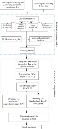
In this study, to determine the best GCMs for climate change projection, GCMs are evaluated with univariate and multivariate statistical approaches. This evaluation is performed based on two variables: rainfall and temperature. Since these two meteorological variables are the most widely used, they are applied to calculate meteorological drought indices. Determining the highest-ranked GCMs will make it possible to calculate hydrological drought indices based on the runoff modelling carried out with IHACRES. Finally, the Bayesian approach is applied to evaluate the uncertainty inherent in climate change projections.

Bias correction data

GCM outputs mostly consist of significant biases, such as modelling very high temperatures, resulting in high or low precipitation, changing rainfall period significantly, and overestimating rainy days. These biases may be caused by large special resolution and a lack of sufficient information about the Earth’s climate (Maraun and Widmann 2018). In previous studies, various approaches were developed and applied for bias correction, such as linear scaling, empirical quantile mapping, and gamma quantile mapping (Mendez et al. 2020). Different bias correction data can be classified based on whether the statistics of the projection period are considered or whether cumulative probability is needed (Watanabe et al. 2012).

In this study, the empirical quantile mapping (EQM) method is applied. This method aims to correct the GCM outputs and coordinate them with the observed climate variable data. To satisfy this objective, a transfer function can be used. As shown in Equations (1)(1) ${P_{contr}}^{\prime }\left(t\right)=CD{F}_{obs,m}^{-1}\left(CD{F}_{conr,m}\left(P_{contr}\left(t\right)\right)\right)$(1) and (2(2) ${P_{ftc}}^{\prime }\left(t\right)=CD{F}_{obs,m}^{-1}\left(CD{F}_{ftc,m}\left(P_{ftc}\left(t\right)\right)\right)$(2) ), this method uses the transfer function to map the GCM outputs to the observation data by the application of cumulative distribution functions (CDFs):

(1) ${P_{contr}}^{\prime }\left(t\right)=CD{F}_{obs,m}^{-1}\left(CD{F}_{conr,m}\left(P_{contr}\left(t\right)\right)\right)$(1)

(2) ${P_{ftc}}^{\prime }\left(t\right)=CD{F}_{obs,m}^{-1}\left(CD{F}_{ftc,m}\left(P_{ftc}\left(t\right)\right)\right)$(2)

where ${P_{contr}}^{\prime }\left(t\right)$ is the bias-corrected data in the control period, $P_{contr}\left(t\right)$ is the projected climate data in the control period, ${P_{ftc}}^{\prime }\left(t\right)$ is the bias-corrected data in the projection period, and $P_{ftc}\left(t\right)$ is the simulated data in the projection period (Mendez et al. 2020).

By applying EQM, the statistical parameters’ mean and standard deviation will be corrected for the GCM output. In this study, the normal distribution is used for correcting temperature data, and gamma distribution is applied to correct the precipitation data. According to previous studies, two-parameter gamma distribution performs adequately in mapping precipitation data (Piani et al. 2010, Watanabe et al. 2012, Leys et al. 2013).

In this study, bias correction is used in two steps: in the control period, to prepare precipitation and temperature data for selecting high-ranked models; and after models are selected, to prepare the corrected GCM outputs for the projection period.

Ranking of simulation models

In this study, the performance of models is evaluated by applying univariate and multivariate statistical approaches. Models are awarded a score of 1–5 based on their ability to simulate precipitation and temperature data for a historical period. Then, models are classified according to their ability to produce the same statistical characteristics as those exhibited by the observed data, and there is no direct comparison between the observed data and the model outputs. The higher ability of a model to reproduce these characteristics leads to it being awarded a higher score.

Univariate methods are widely used because of their simplicity and their ability to provide information about central tendencies and distribution of data, as well as to distinguish the presence or absence of significant trends in data. The methods used in this study are the mean, standard deviation, coefficient of variation, Mann-Kendall (M-K) test, and Kolmogorov-Smirnov (K-S) test.

The mean and standard deviation indicate the central tendency of data and the distribution of data around the central point. The coefficient of variation, defined as the ratio of the standard deviation to the mean, expresses the rate of change per unit of the mean, and it is only applicable to relative scales.

The M-K test is a nonparametric test used to detect monotonic trends in environmental, climate, and hydrological data series. The hypothesis of this test is the randomness (lack of a trend) in the data series, and the rejection of this hypothesis signifies the existence of a trend in the data series. Further details regarding this test can be studied in Pohlert (2016).

The K-S test is a commonly used nonparametric method for comparing two samples to determine whether they are derived from the same population with a specific distribution. This test measures the distance between the empirical distribution function of the sample and the cumulative distribution function of the reference distribution, under the hypothesis that the two samples belong to the same distribution. The K-S test is a distribution-independent test operating based on the maximum vertical distance between the cumulative distribution functions of two samples (Lopes 2011). In this study, the two-sample K-S test is performed on the samples of GCM outputs and observed data, and the results are used to rank the models.

Multivariate analysis refers to any statistical technique for the analysis of data derived from more than one variable. Multivariate analysis can provide a summary or general overview of multivariate data and detect the dominant patterns in the data. The multivariate analysis method used in this study is principal component analysis (Smith 2002).

The scores awarded to each model by the univariate and multivariate analyses of rainfall and temperature variables are averaged to obtain a score for each variable. These two scores are summed to obtain a final score. Of the 26 models assessed, the 14 models with the highest scores are selected for use in later stages.

Since rainfall and temperature data of the models are given at the grid points but observed data are available at the station points, interpolation should be performed to transfer the model data to the station locations. This interpolation is carried out using the inverse distance weighting (IDW) method. This method works under the assumption that the effect of a phenomenon decreases with distance, or, in other words, the value of a continuous variable at a given point is more similar to the values at nearby points than to those at points farther away. In this study, distances are used as the weights of the known variable in predicting unknown points. In this study, after extracting the monthly precipitation and temperature data of each station, the distance of the station points from the four points of the surrounding grid in the modelling network is calculated. Then values of the variables are calculated using the following equation:

(3) $V_{st}=\frac{{\sum }_{i=1}^4\frac{V_i}{d_i}}{{\sum }_{i=1}^4\frac{1}{d_i}}$(3)

where V_st is the desired variable value (precipitation or temperature) at the station coordinates, i is the variable value at four points of the grid that surround the station, and d_i is the station distance to each of the four points.

Following the ranking of models, the variable data are downscaled, and then the daily rainfall and temperature time series of each model, and each scenario can be obtained. In this study, the Long Ashton research station weather generator (LARS-WG) model, a stochastic weather generator, is used for this purpose. The LARS-WG model can generate a time series of weather data for an area under current and future conditions. In this model, the outputs of GCMs have been downscaled with statistical methods in a way that the results are very close to real values. This model consists of three phases: calibration, validation, and generation of weather data for a future period.

In the calibration phase, the collected precipitation and temperature data should be transformed into input files, and the model needs to be run for the base period. Since the LARS-WG model is a stochastic generation model, the model outputs change with each run. Therefore, the model should be run multiple times, and the parameters should be given different weights until the error is minimized (Semenov et al. 2002).

Drought assessment

Many of the drought measurement criteria are based exclusively on analysing variables such as precipitation and temperature. This study uses SPI and SRI indices to assess both meteorological and hydrological droughts. To evaluate the hydrological drought, hydrological variables such as runoff are needed. Thus the runoff flow is modelled in the study area. Here, the IHACRES model is used for this purpose. The IHACRES model consists of a linear loss module and a nonlinear hydrograph module. First, the nonlinear module converts the precipitation and temperature of each time step to the effective rainfall. Then the linear module converts the effective rainfall of that time step into the surface runoff (Jakeman et al. 1990). The regional-scale precipitation and temperature data that were projected under each scenario can be used to calculate the drought indices.

Standardized precipitation and runoff indices

The standardized precipitation index (SPI) was developed by Mckee et al. (1993) for describing and monitoring droughts. To obtain SPI, a probability density function must be fitted to the total precipitation at stations. This is done using the gamma distribution function. For further studies, readers are referred to Livada and Assimakopoulos (2007). The standardized runoff index (SRI) is similar to SPI, with the difference that monthly precipitation is replaced with monthly runoff. More specifically, SRI has been defined as the unit standard normal deviation associated with the percentile of hydrologic runoff accumulated over a specific period. This index can be calculated for different periods (e.g. 1 month or 9 months) and different spatial densities, depending on the application. After calculating the drought indices, the class of the climate is determined based on the classification given in Table 1.

Table 1. The Standardized Runoff Index (SRI) and Standardized Precipitation Index (SPI) drought category classification (Mckee et al. 1993)

Category	SPI and SRI value
Extremely wet	2.0 and above
Very wet	1.5 to 1.99
Moderately wet	1.00 to 1.49
Near normal	−0.99 to 0.99
Moderately dry	−1.0 to −1.49
Severely dry	−1.5 to −1.99
Extremely dry	−2.0 and less

Uncertainty assessment

In climate change studies, there is always a degree of uncertainty induced by the limited accuracy of GCMs, associated with the emission scenario, and caused by spatial and temporal impacts of natural factors on climate change. One of the approaches to consider the model uncertainty is to use the Bayesian method, which operates by the probabilistic representation of uncertainty in model parameters. Using this method, it is also possible to provide a probability distribution for the future climate (Raje and Mujumdar 2010).

In the Bayesian approach, the uncertainty in the parameters of a statistical model is addressed by treating these parameters as random variables. This approach defines a prior probability distribution for parameters, or uses a normal distribution if there is no information available about the prior distribution. If $\theta$ is the vector of model parameters, $p\left(\theta \right)$ is their prior distribution, and $p\left(x|\theta \right)$ is the probability of occurrence of x under the assumptions considered for the model, then the posterior distribution of $\theta$ according to Bayesian theory is expressed by Equation (4):

(4) $p\left(\theta |x\right)=\frac{p\left(x|\theta \right).p\left(\theta \right)}{{\int }_0^{1}p\left(x|\theta \right).p\left(\theta \right)d\theta }$(4)

In most cases, $p\left(x\right)$ does not have a closed-form expression, but if the prior distribution of θ is known, there will be no need to calculate $p\left(x\right)$ directly. In this study, the data are considered equivalent to the SPI classifications obtained from the precipitation projections based on each GCM combination. This dataset is discrete, and its classes are members of the set θ = {extreme drought, severe drought, moderate drought, normal, moderate wetness, severe wetness, extreme wetness}.

After calculating the drought indices for each station over the projection period, the number of occurrences of each drought index class for each model and each scenario is evaluated. Finally, the probability of each of the different classes of the drought indices is calculated.

Study area

Karkheh River is one of the largest and most important rivers in the Persian Gulf and the Oman Sea basin. This river is the confluence of many streams in the Iranian provinces of Ilam, Kermanshah, Lorestan, Hamedan, Kurdistan, and Khuzestan, and finally flows into Hoor al-Azim wetland. The data recorded at meteorological stations over 30 years show variations in climatic variables such as precipitation and temperature in this basin, which reflect the effect of climate change in this region. Therefore, it is crucial to project the impacts of climate change on the probability of certain hydrological phenomena, such as drought, in this region.

The Karkheh basin is located between latitudes 30°58′ and 35°00′N and between longitudes 46°06′ and 49°10′E (Fig. 2). It has an area of about 51 400.8 km², 59% of which is covered by mountainous terrain (mostly in the northern and southern parts); the remaining 41% is covered by plains and foothills. In Fig. 2, six meteorological stations – Aqa Jan Bolaghi, Ahvaz, Dezful, Kermanshah, Khoramabad and Tangeh – and Jelogir hydrometry station located in the study area are shown.

Figure 2. Location of the Karkheh River basin in Iran

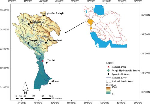
The Karkheh basin has an annual average precipitation of about 350 mm. In recent years, due to significant variations in precipitation and other atmospheric variables such as evaporation and temperature, it has become necessary to investigate the projection of drought occurrences in the future. Because of the combined effects of intensive sunlight, hot and dry winds, and a lack of precipitation in the southern parts of the basin, the evaporation in this region is about 3000 mm per year. In the north of the basin, the geographic and terrain structure reduces the evaporation to less than half of this amount. This has led to the formation of a diverse climate and, consequently, diverse forms of vegetation and activity in the basin.

The mean temperature and monthly rainfall data of the Karkheh basin for the historical period 1971–2005 and the forthcoming period 2020–2049 under scenarios RCP 2.6, RCP 4.5, and RCP 8.5 were collected from 26 GCMs, as shown in Table 2. In RCP2.6, the low global emission scenario, the temperature is assumed to rise by 0.9–2.3°C by 2090. In RCP4.5, the medium global emission scenario, the temperature is assumed to rise by 1.7–3.2°C by 2090. In RCP8.5, the high global emission scenario, the temperature is assumed to rise by 3.2–5.4°C by 2090.

Table 2. The 26 GCMs used in this study

Number	Model	Source
1	bcc-csm-1-1	Beijing Climate Center (BCC), China Meteorological Administration, China
2	bcc-csm1-1-m	Beijing Climate Center (BCC), China Meteorological Administration, China
3	BNU-ESM	GCESS, BNU, Beijing, China
4	CCSM4	Canadian Centre for Climate Modelling and Analysis, Victoria, BC, Canada
5	CESM1-CAM5	NCAR (National Center for Atmospheric Research), Boulder, CO, USA
6	CNRM-CM5	CNRM (Centre National de Recherches Meteorologiques, Meteo-France, Toulouse,France) and CERFACS (Centre Europeen de Recherches et de Formation Avancee en Calcul Scientifique), Toulouse, France
7	CSIRO-Mk3	Australian Commonwealth Scientific and Industrial Research Organization (CSIRO) Marine and Atmospheric Research (Melbourne, Australia) in collaboration with the Queensland Climate Change Centre of Excellence (QCCCE), Brisbane, Australia
8	EC-EARTH	European Community Earth-System
9	FGOALS-g2	IAP (Institute of Atmospheric Physics, Chinese Academy of Sciences, Beijing, China) and THU (Tsinghua University)
10	FIO-ESM	FIO (The First Institution of Oceanography, SOA, Qingdao, China)
11	GFDL-CM3	NOAA GFDL (201 Forrestal Rd, Princeton, NJ, 08540)
12	GFDL-ESM2G	NOAA GFDL (201 Forrestal Rd, Princeton, NJ, 08540)
13	GFDL-ESM2M	NOAA GFDL (201 Forrestal Rd, Princeton, NJ, 08540)
14	GISS-E2-H	Met Office Hadley Centre
15	GISS-E2-R	IPSL (Institut Pierre Simon Laplace, Paris, France)
16	HadGEM2-AO	IPSL (Institut Pierre Simon Laplace, Paris, France)
17	IPSL-CM5A-LR	IPSL (Institut Pierre Simon Laplace, Paris, France)
18	IPSL-CM5A-MR	IPSL (Institut Pierre Simon Laplace, Paris, France)
19	MIROC5	JAMSTEC (Japan Agency for Marine-Earth Science and Technology, Kanagawa, Japan), AORI (Atmosphere and Ocean Research Institute, The University of Tokyo, Chiba, Japan), and NIES (National Institute for Environmental Studies, Ibaraki, Japan)
20	MIROC-ESM	JAMSTEC (Japan Agency for Marine-Earth Science and Technology, Kanagawa, Japan), AORI (Atmosphere and Ocean Research Institute, The University of Tokyo, Chiba, Japan), and NIES (National Institute for Environmental Studies, Ibaraki, Japan)
21	MIROC-ESM-CHEM	JAMSTEC (Japan Agency for Marine-Earth Science and Technology, Kanagawa, Japan), AORI (Atmosphere and Ocean Research Institute, The University of Tokyo, Chiba, Japan), and NIES (National Institute for Environmental Studies, Ibaraki, Japan)
22	MPI-ESM-LR	Max Planck Institute for Meteorology
23	MPI-ESM-MR	Max Planck Institute for Meteorology
24	MRI-CGCM3	MRI (Meteorological Research Institute, Tsukuba, Japan)
25	NorESM1-M	Norwegian Climate Centre
26	NorESM1-ME	Norwegian Climate Centre

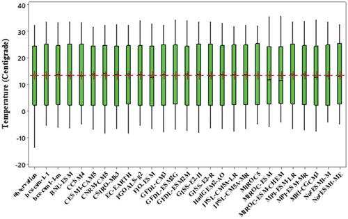
In this study, GCM outputs without any correction consist of biases because most models have overestimated the rainfall before bias correction. Therefore, the EQM method is applied to correct the GCM outputs and coordinate these outputs with the observed climate data. This decreases the distance between the historical (precipitation and temperature) data and the GCM outputs for the period 1971–2005. The box charts of monthly precipitation and temperature from observed data vs. the 26 GCMs for the historical period 1971–2005, after bias correction, are plotted in Figs 3 and 4. Since certain months of the year have zero precipitation, for most models, the median precipitation is close to zero, and therefore many data points fall outside the range. Also as shown in these figures, the monthly temperature variation is closer than the monthly precipitation varation to the historical values.

Figure 3. Box charts of the monthly precipitation according to the 26 GCMs and the observed data for the historical period 1971–2005

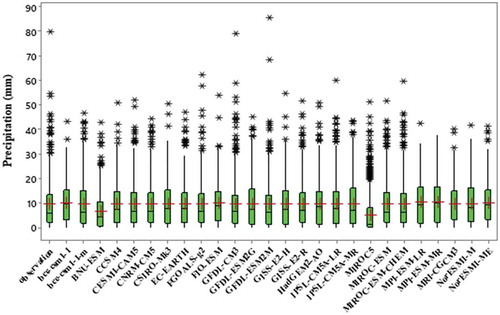
Figure 4. Box charts of the monthly temperature according to the 26 GCMs and the observed data for the historical period 1971–2005

Results

In the following section, the results of single and multicriteria statistical methods for ranking models are presented. Then results of SPI and SRI indices are expressed and, finally, uncertainties in the drought indices are presented.

Model selection

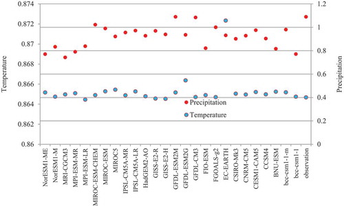
After collecting and analysing precipitation and temperature data for GCMs, the models were ranked. For this purpose, first, the mean and coefficient of variation of GCM outputs and observed data were compared. This comparison showed that for the precipitation, bcc-csm1-1-m, CESM1-CAM5, CSIRO-Mk3, FGOALS-g2, GFDL-ESM2M, and MIROC-ESM-CHEM produced means and standard deviations closest to those of the observed data (Fig. 5). Comparing the coefficient of variation of temperature data (Fig. 6) indicated that the results of all models are quite similar to the historical values.

Figure 5. Comparison of the mean and coefficient of variation for the GCM outputs and the observed precipitation and temperature data

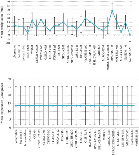
Figure 6. Comparison of the coefficient of variation for the observed precipitation and temperature data and the GCM data

In addition to the mean and coefficient of variation, the results of the M-K and K-S tests were also used as ranking criteria. In the case of the M-K test, the scores awarded to the models were based on the z statistic and p value. The p and z values calculated for each model based on the trend detection of precipitation and temperature data are presented in Table 3. Models IPSL-CM5A-LR and MRI-CGCM3 for precipitation, and models GISS-E2-H, GISS-E2-R, and MPI-ESM-MR for temperature, obtained the z values closest to that of the observed data, and lower p values. The results of the K-S test for precipitation and temperature are presented in Table 3. As can be seen, models FGOALS-g2, CESM1-CAM5, MIROC-ESM, and MIROC-ESM-CHEM for precipitation, and models bcc-csm1-1-m, GISS-E2-H, and CSIRO-Mk3 for temperature, had the lowest K-S statistics and thus were awarded the highest score.

Table 3. The results of Mann-Kendall (M-K) and Kolmogorov-Smirnov (K-S) tests for ranking GCMs

Model	M-K				K-S
	Precipitation		Temperature
	p value	z	p value	z	Precipitation	Temperature
observation	0.168	−1.53	0.453	2.70	0	0
bcc-csm-1-1	0.261	−2.05	0.169	3.89	0.15	0.056
bcc-csm1-1-m	0.732	0.37	0.262	4.06	0.06	0.040
BNU-ESM	0.301	−0.60	0.56	1.39	0.31	0.054
CCSM4	0.339	−0.45	0.244	3.86	0.09	0.061
CESM1-CAM5	0.299	0.43	0.269	3.98	0.05	0.049
CNRM-CM5	0.774	−0.57	0.73	0.77	0.07	0.049
CSIRO-Mk3	0.565	0.57	0.31	3.92	0.10	0.043
EC-EARTH	0.813	0.62	0.594	1.25	0.09	0.068
FGOALS-g2	0.845	−0.31	0.486	2.61	0.04	0.056
FIO-ESM	0.513	1.39	0.561	2.33	0.13	0.061
GFDL-CM3	0.924	0.48	0.268	2.24	0.06	0.056
GFDL-ESM2G	0.947	−0.37	0.337	2.90	0.09	0.068
GFDL-ESM2M	0.413	−0.91	0.361	2.67	0.08	0.061
GISS-E2-H	0.864	0.74	0.393	2.67	0.10	0.042
GISS-E2-R	0.304	1.16	0.779	0.65	0.07	0.061
HadGEM2-AO	0.213	−1.19	0.128	3.69	0.13	0.051
IPSL-CM5A-LR	0.343	−1.53	0.152	4.03	0.12	0.049
IPSL-CM5A-MR	0.488	−2.10	0.272	3.89	0.09	0.058
MIROC5	0.864	2.67	0.333	2.78	0.69	0.061
MIROC-ESM	0.922	1.08	0.443	2.56	0.05	0.085
MIROC-ESM-CHEM	0.478	−0.74	0.342	3.41	0.05	0.104
MPI-ESM-LR	0.206	−1.02	0.272	3.15	0.15	0.054
MPI-ESM-MR	0.503	1.22	0.303	2.76	0.18	0.064
MRI-CGCM3	0.178	−1.62	0.442	2.27	0.18	0.083
NorESM1-M	0.154	1.73	0.602	1.56	0.12	0.048
NorESM1-ME	0.577	0.85	0.354	3.47	0.17	0.054

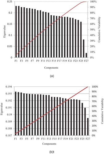
In addition to univariate tests, the results of a multivariate test known as principal component analysis (PCA) were used to rank the GCMs. The results of the PCA are illustrated in Fig. 7. This analysis was performed on observed data and GCM outputs, which together constituted 27 principal components. The local variance between model outputs and observed data in the first component was used to score the models.

Figure 7. Results of the PCA for observed data and model outputs. (a) Precipitation data; (b) temperature data

The scores awarded to each model in each evaluation for precipitation and temperature data are listed in Tables 4 and 5. Finally, the models were ranked based on these scores, and the 14 models with the highest ranks were chosen, as shown in Table 6.

Table 4. The scores awarded to each model for precipitation data

Number	Model	Mean	Standard deviation	Coefficient of variation	Mann- Kendall test	Kolmogrov-Smirnov test	Principal Component Analysis (PCA)
1	bcc-csm1-1	4.71	3.94	1.33	4.06	4.51	4.49
2	bcc-csm1-1-m	4.99	4.58	3.74	5.00	3.19	3.88
3	BNU-ESM	2.14	2.20	4.99	4.11	4.11	2.67
4	CCSM4	4.97	4.30	2.86	3.67	3.97	4.71
5	CESM1-CAM5	4.99	4.57	3.68	4.42	3.14	5.00
6	CNRM-CM5	5.00	4.37	3.14	4.41	4.08	4.11
7	CSIRO-Mk3	4.95	4.31	2.83	4.82	3.00	4.18
8	EC-EARTH	4.97	4.40	3.17	3.23	2.95	4.04
9	FGOALS-g2	4.99	4.65	3.97	3.97	3.84	4.59
10	FIO-ESM	4.85	4.05	1.90	3.67	2.22	4.71
11	GFDL-CM3	5.00	5.00	4.94	3.97	3.08	3.48
12	GFDL-ESM2G	4.98	4.42	3.23	3.23	3.89	3.69
13	GFDL-ESM2M	4.97	4.98	5.00	3.66	4.41	3.62
14	GISS-E2-H	5.00	4.41	3.26	4.86	2.84	3.73
15	GISS-E2-R	5.00	4.53	3.61	3.67	2.43	4.54
16	HadGEM2-AO	4.97	4.39	3.13	4.29	4.68	3.88
17	IPSL-CM5A-LR	4.91	4.62	3.64	4.46	5.00	3.50
18	IPSL-CM5A-MR	4.91	4.56	3.45	3.88	4.46	3.61
19	MIROC5	1.00	1.00	3.06	3.67	1.00	1.00
20	MIROC-ESM	5.00	4.62	3.85	2.18	2.51	4.86
21	MIROC-ESM-CHEM	5.00	4.75	4.22	1.00	4.24	4.61
22	MPI-ESM-LR	4.63	4.29	2.10	4.12	4.51	3.35
23	MPI-ESM-MR	4.57	4.12	1.55	3.53	2.38	3.35
24	MRI-CGCM3	4.88	3.70	1.00	2.33	4.92	4.80
25	NorESM1-M	4.90	4.07	2.04	4.52	1.89	4.84
26	NorESM1-ME	4.72	3.93	1.32	4.11	2.73	4.70

Table 5. The scores awarded to each model for temperature data

Number	Model	Mean	Standard deviation	Coefficient of variation	Mann- Kendall test	Kolmogrov-Smirnov test	Principal Component Analysis (PCA)
1	bcc-csm1-1	4.58	4.98	4.76	4.00	2.69	2.29
2	bcc-csm1-1-m	4.97	2.18	4.89	5.00	2.35	2.35
3	BNU-ESM	4.82	2.33	4.96	4.00	2.46	1.64
4	CCSM4	4.83	1.00	4.60	3.57	2.75	1.68
5	CESM1-CAM5	4.75	3.01	4.85	4.29	2.52	1.22
6	CNRM-CM5	4.88	1.50	4.94	4.43	1.23	2.41
7	CSIRO-Mk3	4.93	3.88	4.85	4.71	2.63	1.49
8	EC-EARTH	5.00	2.35	4.84	3.29	2.18	1.67
9	FGOALS-g2	4.95	4.97	4.95	4.00	4.89	2.70
10	FIO-ESM	4.82	4.59	4.79	3.57	4.32	2.89
11	GFDL-CM3	4.70	4.39	4.66	4.00	4.15	3.08
12	GFDL-ESM2G	4.79	2.51	4.64	3.29	4.66	2.87
13	GFDL-ESM2M	4.97	4.33	5.00	3.57	5.00	2.95
14	GISS-E2-H	4.34	5.00	4.33	4.86	5.00	3.80
15	GISS-E2-R	4.77	4.86	4.75	3.71	1.00	5.00
16	HadGEM2-AO	4.88	4.68	4.85	4.29	3.08	1.61
17	IPSL-CM5A-LR	4.76	4.86	4.74	4.29	2.41	1.83
18	IPSL-CM5A-MR	1.00	4.74	1.00	3.71	2.69	1.11
19	MIROC5	4.77	2.03	4.93	3.57	4.89	1.00
20	MIROC-ESM	4.94	4.26	4.88	2.14	4.77	2.61
21	MIROC-ESM-CHEM	5.00	4.47	4.98	1.00	3.65	2.89
22	MPI-ESM-LR	4.93	4.48	4.89	4.14	4.15	1.84
23	MPI-ESM-MR	4.93	4.36	4.96	3.57	4.94	2.33
24	MRI-CGCM3	4.94	3.60	4.99	2.29	4.21	1.77
25	NorESM1-M	4.82	4.30	4.76	4.43	2.80	1.58
26	NorESM1-ME	4.77	4.36	4.73	4.00	3.54	1.42

Table 6. Final scores of each GCM for precipitation and temperature data

Number	Model	Precipitation score	Temperature score	Final score	Selection	Number of selected GCMs
1	bcc-csm1-1	3.75	4.49	7.59
2	bcc-csm1-1-m	3.36	3.88	7.59	✓	1
3	BNU-ESM	3.08	2.67	6.45
4	CCSM4	2.72	4.71	6.80
5	CESM1-CAM5	3.18	5.00	7.48	✓	2
6	CNRM-CM5	2.90	4.11	7.09
7	CSIRO-Mk3	3.51	4.18	7.53	✓	3
8	EC-EARTH	2.87	4.04	6.66
9	FGOALS-g2	4.30	4.59	8.64	✓	4
10	FIO-ESM	4.03	4.71	7.60	✓	5
11	GFDL-CM3	4.06	3.48	8.30	✓	6
12	GFDL-ESM2G	3.59	3.69	7.50	✓	7
13	GFDL-ESM2M	4.17	3.62	8.61	✓	8
14	GISS-E2-H	4.60	3.73	8.61	✓	9
15	GISS-E2-R	3.86	4.54	7.83	✓	10
16	HadGEM2-AO	3.70	3.88	7.92	✓	11
17	IPSL-CM5A-LR	3.63	3.50	7.98	✓	12
18	IPSL-CM5A-MR	2.65	3.61	6.80
19	MIROC5	3.28	1.00	5.07
20	MIROC-ESM	3.73	4.86	7.57	✓	13
21	MIROC-ESM-CHEM	3.40	4.61	7.37
22	MPI-ESM-LR	3.90	3.35	7.74	✓	14
23	MPI-ESM-MR	4.03	3.35	7.28
24	MRI-CGCM3	3.37	4.80	6.98
25	NorESM1-M	3.58	4.84	7.29
26	NorESM1-ME	3.61	4.70	7.19

In the next step, IDW interpolation was performed to examine the effects of climate change at the station points and to compare the model data with the observed data. To prepare the data for downscaling, the EQM method was applied for bias correction of GCM outputs for the projection period. Then, utilizing the bias-corrected GCM outputs and the historical data from the meteorological stations, the LARS-WG model was developed to downscale the outputs of the selected models for the stations. The stochastic component of LARS-WG is controlled by a random number seed. In this paper, the alternative random seed number of 541 was used to generate synthetic daily weather for the stations. To compare the projected time series, their monthly precipitation and monthly average temperature values were calculated. Figure 8, for example, displays the future average precipitation values of the Aqa Jan Bolaghi raingauge station under scenarios RCP2.6, RCP 4.5, and RCP8.5 as projected by the 14 selected models.

Figure 8. The monthly precipitation values (2020–2049) projected for Aqa Jan Bolaghi Station by the 14 selected models under scenario (a) RCP2.6, (b) RCP4.5 and (c) RCP8.5

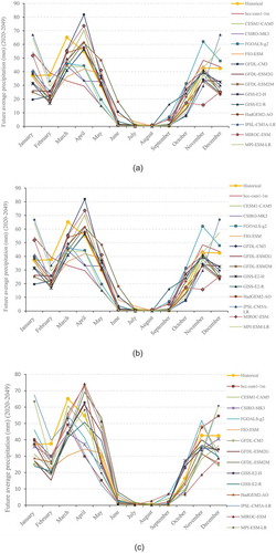
According to historical data, the annual average precipitation at this station is 339 mm. As shown in Fig. 8, the most critical drop in precipitation, 0.79, is related to the model FIO-ESM under scenario RCP8.5, whereas the highest increase in rainfall, 1.01, is related to the model FGOALS-g2 under the scenario RCP2.6.

From the analysis of temperature and precipitation variations in all stations, it can be concluded that there is likely to be a change in the precipitation pattern over the projection period. However, these variations do not have a clear trend; in some stations, the average monthly precipitation will increase in January and decrease in February, whereas in others, the opposite will happen. For rainy months such as February, March, November, and December, the range of changes projected by models is very high, reaching up to 35 mm at some stations. The changes in the temperature trend are uniform, and all models show temperature rise under all three scenarios. For the temperature, the selected models produce more convergent results compared to precipitation, and the difference among the projected values is less than 1°C.

Evaluation of uncertainty in drought indices

To calculate the drought indices, it was first necessary to model the runoff of the study area. The runoff is simulated using the IHACRES model. The runoff data for Jelogir hydrometry station from 1970 to 1985 were used for the model calibration period. Then, the developed model was utilized to simulate the runoff for the projection period.

The precipitation and temperature time series projected based on different models and under three RCP scenarios were entered in the IHACRES model as inputs. Table 7 presents the average changes in minimum and maximum discharges projected for each month for Jelogir hydrometry station. According to these results, over the projection period, the annual average discharge values will decrease by an average of 4%.

Table 7. The average monthly changes in minimum and maximum discharges projected for Jelogir hydrometry station

Month	Minimum projected runoff			Maximum projected runoff			Observed
	Model	Scenario	Average discharge changes	Model	Scenario	Average discharge changes
1	GFDL-CM3	RCP2.6	0.36	bcc-csm-1-1	RCP2.6	1.44	88.33
2	GFDL-CM3	RCP2.6	0.30	IPSL-CM5A-LR	RCP8.5	1.05	152.33
3	MIROC-ESM	RCP2.6	0.51	IPSL-CM5A-LR	RCP8.5	0.98	259.91
4	MIROC-ESM	RCP2.6	0.67	GFDL-ESM2G	RCP4.5	1.05	322.33
5	bcc-csm-1-1	RCP4.5	1.33	GFDL-ESM2M	RCP4.5	1.87	192.67
6	CESM-CAM5	RCP4.5	1.19	GFDL-ESM2M	RCP2.6	2.74	78.58
7	MIROC-ESM	RCP8.5	1.85	FIO-ESM	RCP4.5	2.67	44.58
8	GFDL-ESM2G	RCP4.5	1.48	MIROC-ESM	RCP8.5	2.51	33.92
9	GFDL-ESM2G	RCP4.5	0.79	MIROC-ESM	RCP2.6	2.37	31.50
10	GFDL-ESM2G	RCP4.5	0.39	MIROC-ESM	RCP2.6	1.38	44.50
11	GFDL-CM3	RCP4.5	0.43	HadGEM2-AO	RCP4.5	1.32	78.17
12	GFDL-CM3	RCP8.5	0.40	IPSL-CM5A-LR	RCP4.5	1.20	115.92
Sum	0.76			1.05			1442
Annual average changes				0.96

To evaluate the model uncertainty, the occurrence of each class of the drought index (a series of occurrences or non-occurrences of that class) for each scenario-model combination was assessed. The binomial and beta distributions are considered the representatives of the prior and posterior distributions, respectively.

This approach was repeated for all models and scenarios. Then the probability of occurrence of each class of drought index (extreme drought, severe drought, moderate drought, normal, moderate wetness, severe wetness, extreme wetness) over the projection period is considered as the ratio of occurrence of that class in all models and scenarios. This study consists of 14 models and three scenarios; thus, there were a total of 42 model-scenario combinations. Moreover, drought indices should be calculated for every year of the 30-year projection period. Accordingly, the total number of states in which the occurrence of drought index classes should be examined was 1260. The probability of occurrence in the projection period was obtained by dividing the number of occurrences by the total number of states, and the respective beta distribution for each drought index class for each station was plotted.

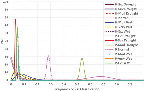
Figure 9 shows the posterior distributions obtained for each SPI class for historical (1971–2005) and projected (2020–2049) data at each station. The derived posterior distributions show the mean value and its variations of SPI frequency for different categories considering the spread and tails of the distribution. The figure shows the mean frequency of normal conditions decreases in the future at all stations, and that of moderate and severe drought conditions increases in future. Table 8 shows the mean and standard deviation of the occurrence probability of different SPI classes for meteorological stations for the historical (1971–2005) and future (2020–2049) time series data.

Table 8. Mean and standard deviation of the probability of SPI classes for the stations

Years	Standardized precipitation index (SPI) Classification	Extreme drought	Severe drought	Moderate drought	Normal	Moderate wet	Very wet	Extreme wet
Aqa Jan Bolaghi Station
1971–2005	Mean freq.	0.034	0.034	0.103	0.655	0.138	0.034	0.000
	Std dev of freq.	0.033	0.033	0.056	0.087	0.063	0.033	0.000
2020–2049	Mean freq.	0.020	0.039	0.101	0.341	0.465	0.067	0.007
	Std dev of freq.	0.004	0.005	0.008	0.014	0.013	0.007	0.002
Ahwaz Station
1971–2005	Mean freq.	0.000	0.086	0.029	0.771	0.057	0.029	0.029
	Std dev of freq.	0.000	0.047	0.028	0.070	0.039	0.028	0.028
2020–2049	Mean freq.	0.021	0.047	0.104	0.333	0.45	0.044	0.000
	Std dev of freq.	0.004	0.006	0.008	0.013	0.014	0.006	0.000
Dezful Station
1971–2005	Mean freq.	0.032	0.000	0.065	0.677	0.097	0.097	0.032
	Std dev of freq.	0.031	0.000	0.043	0.083	0.052	0.052	0.031
2020–2049	Mean freq.	0.036	0.047	0.095	0.289	0.522	0.011	0.000
	Std dev of freq.	0.005	0.006	0.008	0.012	0.014	0.029	0.000
Kermanshah Station
1971–2005	Mean freq.	0.029	0.000	0.171	0.615	0.114	0.057	0.029
	Std dev of freq.	0.028	0.000	0.063	0.082	0.053	0.039	0.028
2020–2049	Mean freq.	0.02	0.071	0.078	0.382	0.4	0.031	0.017
	Std dev of freq.	0.004	0.007	0.007	0.014	0.014	0.005	0.004
Khoramabad Station
1971–2005	Mean freq.	0.030	0.030	0.152	0.697	0.030	0.030	0.030
	Std dev of freq.	0.029	0.029	0.061	0.079	0.029	0.029	0.029
2020–2049	Mean freq.	0.047	0.036	0.055	0.351	0.049	0.022	0.000
	Std dev of freq.	0.006	0.005	0.006	0.013	0.014	0.004	0.000
Tangeh Station
1971–2005	Mean freq.	0.061	0.000	0.091	0.727	0.091	0.061	0.030
	Std dev of freq.	0.039	0.000	0.047	0.077	0.047	0.039	0.028
2020–2049	Mean freq.	0.044	0.032	0.084	0.330	0. 467	0.032	0.009
	Std dev of freq.	0.006	0.005	0.008	0.013	0.014	0.005	0.003

Figure 9. The posterior distributions of SPI classes for historical and projected data at the following stations: (a) Aqa Jan Bolaghi; (b) Ahvaz; (c) Dezful; (d) Kermanshah; (e) Khoramabad; (f) Tangeh

H- Historical; P- Projection; Ext- Extreme; Mod- Moderate; Sev- Severe.

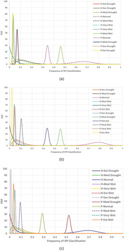
Figure 9. Continued

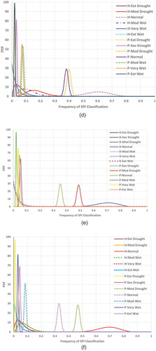
The expected frequencies for each SPI classification obtained from the posterior distribution of Bayesian analysis for historical and projected data of the entire basin are presented in Fig. 10. According to this figure, the highest occurrence probability is related to the normal condition. The trend from 1971–2005 to 2020–2049 shows an increased probability of moderate drought and the simultaneous increasing probability of normal conditions. The trend appears to be insignificant for wet conditions.

Figure 10. Expected values for frequencies of SPI classifications obtained from posterior distribution of Bayesian analysis

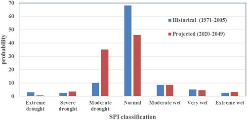
The posterior distributions obtained for SRI classes in the historical and projected periods for Jelogir hydrometry station are plotted in Fig. 11. As this figure shows, the highest occurrence probability for the period 2020–2049 is 0.537 and belongs to the moderate dry condition. The next most probable state is near normal, with an average probability of 0.282. Table 9 shows the mean and standard deviation of the probability of occurrence of each SRI class.

Table 9. Mean and standard deviation of the probability of Standardized Runoff Index (SRI) classes

Category	1971–2005		2020–2049
	Mean	Standard deviation	Mean	Standard deviation
Extremely wet	0.033	0.032	0.006	0.048
Very wet	0.033	0.032	0.006	0.048
Moderately wet	0.033	0.032	0.006	0.05
Near normal	0.667	0.085	0.013	0.282
Moderately dry	0.100	0.054	0.014	0.537
Severely dry	0.067	0.045	0.005	0.035
Extremely dry	0.067	0.045	0	0

Figure 11. The posterior distributions obtained for SRI classes for historical and projected data

H- Historical; P- Projection; Ext- Extreme; Mod- Moderate; Sev- Severe.

As these results indicate, for all studied stations in the Karkheh basin, the most probable state is the occurrence of the near-normal condition (as defined based on the definition of meteorological and hydrological drought) with a probability of 46% for projected data. The trend from historical to projected data shows an increased probability of dry conditions and the simultaneous increasing probability of normal conditions.

Conclusion

In this study, to investigate the impacts of climate change on extreme climate indices such as meteorological and hydrological droughts, certain variables including temperature, precipitation, and runoff are projected for the future period. The following steps were applied to evaluate the impacts of climate change on drought characteristics in Karkheh basin:

• The available precipitation and temperature outputs of 26 GCMs under three RCP scenarios were collected and compared with a set of observed data.

• The empirical quantile mapping (EQM) method was applied for bias correction. It was used in two steps: firstly, in the control period (1971–2005), to prepare precipitation and temperature data for selecting high-ranked models, which reduced the distance between observed data and GCM outputs; and, secondly, after model selection, to correct GCM outputs for the projection period (2020–2049) for each station.

• To determine the best models for climate change modelling in the study area, each model was scored and ranked based on the criteria. Single statistical criterion tests including mean and standard deviation, coefficient of variation, Mann-Kendall, and Kolmogorov-Smirnov, and a multivariate criterion test, using the principal component obtained from PCA, were used.

• After ranking the models, the models bcc-csm1-1 m, CESM1-CAM5, CSIRO-MK3, FGOALS-g2, FIO-ESM, GFDL-CM3, GFDL-ESM2G, GFDL-ESM2M, GISS-E2-H, GISS-E2-R, HadGEM2-AO, IPSL-CM5A-LR, MIROC-ESM, and MPI-ESM-LR, which earned an average score of over 7.48 for both precipitation and temperature, were identified as the most suitable models for simulating climate change impacts in the study area.

• The climate scenarios produced by these models were used in the LARS downscaling model to obtain the precipitation and temperature time series for the projection period. The projected time series was utilized in the hydrologic model IHACRES to obtain the runoff time series for the projection period.

• The precipitation projection results indicated a change in the precipitation pattern. They showed an annual average precipitation variation of at least 0.79 in the FIO-ESM model and at most 1.01 in the FGOALS-g2 model. However, a dramatic change in the precipitation of the entire basin is not likely. On average, the temperature of the basin as a whole is set to increase by about 1°C by 2049. The SPI and SRI drought indices were used to assess the probability of meteorological and hydrological droughts using the projected precipitation and runoff time series.

• Finally, the Bayesian approach was used to model the uncertainty to assess drought occurrence. For this purpose, the occurrence of each class of the drought indices was estimated using a binomial distribution. Then the Bayesian theory was utilized to obtain the posterior distribution of occurrence of the different index classes. The results showed that the most probable state for all studied stations is the moderately dry condition, with a probability of 54% and a standard deviation of 1.4%, and the next most probable state is a near normal condition.

In this study, a watershed in Iran was considered as a case study. This approach can be applied in other watersheds to project climate change and assess the uncertainty based on the proposed methodology. Although it may have high computational cost, this methodology can be used in catchments and can be considered in larger case studies to simulate precipitation and temperature changes. Moreover, runoff can be simulated by applying other rainfall-runoff models or through the application of data-driven methods.

Acknowledgements

The authors thank the two anonymous reviewers for their very insightful comments and suggestions that were helpful in improving this paper.

Disclosure statement

No potential conflict of interest was reported by the authors.

References

- Bates, B., et al. 2008. Climate change and water. Technical paper of the intergovernmental panel on climate change, Geneva: IPCC Secretariat, 210.
- Bergthorsson, P., et al., 1988. The effects of climatic variations on agriculture in Iceland. The Impact of Climatic Variations on Agriculture, 1, 381–509.
- Beyene, T., Lettenmaier, D.P., and Kabat, P., 2010. Hydrologic impacts of climate change on the Nile River Basin: implications of the 2007 IPCC scenarios. Climatic Change, 100 (3–4), 433–461. doi:10.1007/s10584-009-9693-0
- Carter, T., et al., 2007. General guidelines on the use of scenario data for climate impact and adaptation assessment. Helsinki, Finland: Finnish Environmental Institute.
- Chen, J., Brissette, F.P., and Leconte, R., 2011. Uncertainty of downscaling method in quantifying the impact of climate change on hydrology. Journal of Hydrology, 401 (3–4), 190–202. doi:10.1016/j.jhydrol.2011.02.020
- Dai, A., Trenberth, K.E., and Qian, T., 2004. A global dataset of Palmer Drought Severity Index for 1870–2002: relationship with soil moisture and effects of surface warming. Journal of Hydrometeorology, 5 (6), 1117–1130. doi:10.1175/JHM-386.1
- Duan, K. and Mei, Y., 2014. Comparison of meteorological, hydrological and agricultural drought responses to climate change and uncertainty assessment. Water Resources Management, 28 (14), 5039–5054. doi:10.1007/s11269-014-0789-6
- Giorgi, F., et al., 2001. Regional climate information—evaluation and projections. Geological and Atmospheric Sciences Publications, 110. Available from: https://lib.dr.iastate.edu/ge_at_pubs/110
- Hanewinkel, M., et al., 2013. Climate change may cause severe loss in the economic value of European forest land. Nature Climate Change, 3 (3), 203. doi:10.1038/nclimate1687
- Hardy, J.T., 2003. Climate change: causes, effects, and solutions. Hoboken, New Jersey: John Wiley & Sons.
- Hellström, C. and Chen, D., 2003. Statistical downscaling based on dynamically downscaled predictors: application to monthly precipitation in Sweden. Advances in Atmospheric Sciences, 20 (6), 951–958. doi:10.1007/BF02915518
- Hillel, D. and Rosenzweig, C. 1988. The greenhouse effect and its implications regarding global agriculture. In: Research Bulletin/Massachusetts Agricultural Experiment Station (USA). College of Food and Natural Resources, 724.
- Jakeman, A., Littlewood, I., and Whitehead, P., 1990. Computation of the instantaneous unit hydrograph and identifiable component flows with application to two small upland catchments. Journal of Hydrology, 117 (1–4), 275–300. doi:10.1016/0022-1694(90)90097-H
- Kattsov, V.M., et al., 2005. Future climate change: modeling and scenarios for the Arctic. In: Arctic Climate Impact Assessment (ACIA). Cambridge, UK: Cambridge University Press, 99–150
- Kudo, R., Yoshida, T., and Masumoto, T., 2017. Uncertainty analysis of impacts of climate change on snow processes: case study of interactions of GCM uncertainty and an impact model. Journal of Hydrology, 548, 196–207. doi:10.1016/j.jhydrol.2017.03.007
- Lee, J.-K. and Kim, Y.-O., 2017. Selection of representative GCM scenarios preserving uncertainties. Journal of Water and Climate Change, 8 (4), 641–651. doi:10.2166/wcc.2017.101
- Leys, C., et al., 2013. Detecting outliers: do not use standard deviation around the mean, use absolute deviation around the median. Journal of Experimental Social Psychology, 49 (4), 764–766. doi:10.1016/j.jesp.2013.03.013
- Liuzzo, L., et al., 2009. Basin-scale water resources assessment in Oklahoma under synthetic climate change scenarios using a fully distributed hydrologic model. Journal of Hydrologic Engineering, 15 (2), 107–122. doi:10.1061/(ASCE)HE.1943-5584.0000166
- Livada, I. and Assimakopoulos, V., 2007. Spatial and temporal analysis of drought in Greece using the Standardized Precipitation Index (SPI). Theoretical and Applied Climatology, 89 (3–4), 143–153. doi:10.1007/s00704-005-0227-z
- Lopes, R.H., 2011. Kolmogorov-smirnov test. vol. 2011. Berlin: Springer, 718–720.
- Maraun, D. and Widmann, M., 2018. Statistical downscaling and bias correction for climate research. Cambridge, UK: Cambridge University Press. doi:10.1017/9781107588783
- Mckee, T.B., Doesken, N.J., and Kleist, J., 1993. The relationship of drought frequency and duration to time scales. In: Proceedings of the 8th Conference on Applied Climatology, Anaheim, California, 179–183.
- Mearns, L.O., Rosenzweig, C., and Goldberg, R., 1996. The effect of changes in daily and interannual climatic variability on CERES-Wheat: a sensitivity study. Climatic Change, 32 (3), 257–292. doi:10.1007/BF00142465
- Mendez, M., et al., 2020. Performance evaluation of bias correction methods for climate change monthly precipitation projections over Costa Rica. Water, 12 (2), 482. doi:10.3390/w12020482
- Piani, C., et al., 2010. Statistical bias correction of global simulated daily precipitation and temperature for the application of hydrological models. Journal of Hydrology, 395 (3–4), 199–215. doi:10.1016/j.jhydrol.2010.10.024
- Pohlert, T., 2016. Non-parametric trend tests and change-point detection. CC BY-ND, 4, 1–18.
- Raje, D. and Mujumdar, P., 2010. Hydrologic drought prediction under climate change: uncertainty modeling with Dempster–Shafer and Bayesian approaches. Advances in Water Resources, 33 (9), 1176–1186. doi:10.1016/j.advwatres.2010.08.001
- Rosenberg, N.J., et al., 1993. The MINK methodology: background and baseline. In: Rosenberg N.J., ed. Towards an integrated impact assessment of climate change: the MINK study. Dordrecht: Springer, 7–22.
- Semenov, M.A., Barrow, E.M., and Lars-Wg, A., 2002. A stochastic weather generator for use in climate impact studies. In: User Man Herts UK. User Manual, 1–27. Available from: http://www.rothamsted.ac.uk/mas-models/larswg.php
- Shiklomanov, N.I., et al., 2017. Climate change and stability of urban infrastructure in Russian permafrost regions: prognostic assessment based on GCM climate projections. Geographical Review, 107 (1), 125–142. doi:10.1111/gere.12214
- Smith, L.I., 2002. A tutorial on principal components analysis (Computer Science Technical Report No. OUCS-2002-12). New Zealand: University of Otago. Available from: http://hdl.handle.net/10523/7534
- Sunyer, M.A., et al., 2015. Inter-comparison of statistical downscaling methods for projection of extreme precipitation in Europe. Hydrology and Earth System Sciences, 19 (4), 1827–1847. doi:10.5194/hess-19-1827-2015
- Walton, D.B., et al., 2017. Incorporating snow albedo feedback into downscaled temperature and snow cover projections for California’s Sierra Nevada. Journal of Climate, 30 (4), 1417–1438. doi:10.1175/JCLI-D-16-0168.1
- Watanabe, S., et al., 2012. Intercomparison of bias‐correction methods for monthly temperature and precipitation simulated by multiple climate models. Journal of Geophysical Research: Atmospheres, 117, D23. doi:10.1029/2012JD018192
- Widmann, M., Bretherton, C.S., and Salathé, J.E., 2003. Statistical precipitation downscaling over the northwestern United States using numerically simulated precipitation as a predictor. Journal of Climate, 16 (5), 799–816. doi:10.1175/1520-0442(2003)016<0799:SPDOTN>2.0.CO;2
- Wilby, R.L. and Harris, I., 2006. A framework for assessing uncertainties in climate change impacts: low‐flow scenarios for the River Thames, UK. Water Resources Research, 42 (2). doi:10.1029/2005WR004065
- Wilhite, D.A. and Glantz, M.H., 1985. Understanding: the drought phenomenon: the role of definitions. Water International, 10 (3), 111–120. doi:10.1080/02508068508686328
- Williams, G., et al., 1988. Estimating effects of climatic change on agriculture in Saskatchewan, Canada. Dordrecht, Netherlands: Kluwer Academic Publishers.
- Wood, A.W., et al., 2004. Hydrologic implications of dynamical and statistical approaches to downscaling climate model outputs. Climatic Change, 62 (1–3), 189–216. doi:10.1023/B:CLIM.0000013685.99609.9e