An adaptive daily runoff forecast model using VMD-LSTM-PSO hybrid approach

ABSTRACT

To cope with the nonlinear and nonstationarity challenges faced by conventional runoff forecasting models and improve daily runoff prediction accuracy, a hybrid model-based “feature decomposition-component prediction-result reconstruction” named VMD-LSTM-PSO was proposed. First, variational mode decomposition (VMD) was used to decompose the original daily runoff series into a discrete number of intrinsic mode functions (IMFs) to produce clearer signals. Then, for each IMF, a long short-term memory (LSTM) network was applied to establish the prediction model, and a particle swarm optimization (PSO) algorithm was utilised to optimise the number of hidden layer nodes and the learning rate of the LSTM. The model was applied in three hydrologic stations in the main stream of the Yellow River of China and compared with the complementary ensemble empirical mode decomposition coupled long short-term memory and particle swarm optimization (CEEMD-LSTM-PSO), wavelet transform coupled long short-term memory and particle swarm optimization (WT-LSTM-PSO) and LSTM-PSO models. Based on its high predictive accuracy and stability, the novel model promises to be a preferred data-driven tool for hydrological forecasting in practice.

KEYWORDS:

• daily runoff forecasting
• variational mode decomposition
• long short-term memory network
• climate change
• the Yellow River

Editor A. Fiori Associate Editor F-J. Chiang

1 Introduction

Accurate and reliable daily runoff forecasting is vital for flood control planning, reservoir dispatching, water resource allocation, hydropower station operation, etc. (Xie et al. 2019). However, due to the combined effects of climate, underlying surface conditions and human activities, the daily runoff sequence exhibits typical nonlinear, nonstationary dynamic characteristics and strong correlation, which makes it hard to capture potential change processes effectively through common streamflow forecasting techniques (Zhu et al. 2016). There is still a certain degree of difficulty in achieving high-precision prediction of daily runoff, so further research is needed.

Currently, the methods of runoff prediction can be divided into two categories: process-driven methods and data-driven methods. Process-driven methods are based on the hydrological concept with a physical mechanism, while data-driven methods predict runoff rapidly by acquiring related data without considering the physical mechanism. In recent years, due to the introduction of artificial neural network (ANN) (Humphrey et al. 2016), support vector machine (SVM) (Yaseen et al. 2016), adaptive neuro-fuzzy inference system (ANFIS) (Ashrafi et al. 2017), and grey model (GM) (Yaseen et al. 2018), as well as the development of hydrological data acquisition capabilities and computing capability, data-driven models have been playing a huge role in hydrological forecasting. These methods offer advantages over conventional modelling, including the ability to handle large amounts of noisy data from dynamic and nonlinear systems, especially when the underlying physical relationships are not fully understood (He et al. 2014). ANN in particular is known to mimic highly nonlinear and complex systems well, and is widely used in hydrological fields (Kasiviswanathan et al. 2013, Chang et al. 2015, Humphrey et al. 2016, Shiau and Hsu 2016, Maroufpoor et al. 2019), such as in rainfall forecasting (Hung et al. 2009, Kasiviswanathan et al. 2013), monthly and daily runoff forecasting (Humphrey et al. 2016, Shiau and Hsu 2016), reservoir inflow forecasting (Chang et al. 2015, Yaseen et al. 2019a), urban drainage systems (Chang et al. 2014) and so on. However, traditional ANN and recurrent neural network (RNN) models face some problems, such as overfitting, poor generalizability, the ease of falling into local optimization, gradient disappearance, and gradient explosion in the process of conventional training (Fan et al. 2020, Li et al. 2021). Due to the “shallow” learning mechanism of these models, they have limited ability to address input features and capture long-term correlation of time series, which leads to their poor performance in forecasting streamflow with nonlinear and nonstationary characteristics (Kratzert et al. 2018, Gao et al. 2020, Li et al. 2020).

Recently, researchers have increasingly focused on the application of the long short-term memory (LSTM) in hydrological fields, due to its nonlinear predictive capability, faster convergence and ability to capture long-term correlation of time series. The LSTM architecture is a special kind of RNN, which is designed to overcome the weakness of the traditional RNN to learn long-term dependencies. Kratzert et al. (2018) demonstrated that rainfall-runoff modelling using LSTM achieves better model performance than the well-known Sacramento Soil Moisture Accounting Model (SAC-SMA), which underlines the potential of the LSTM for hydrological modelling applications. Yuan et al. (2018) compared the LSTM with the back propagation (BP) neural network, radial basis neural network (RBNN) and least squares support vector machine (LSSVM) models for monthly runoff forecasting. The results showed that the LSTM model is significantly better than the other three models. Zhang et al. (2018a) found that the LSTM model can effectively reduce the time consumption and memory storage required by the BP neural network and SVM models, and demonstrates good capability in simulating low-flow conditions and the outflow curve for the peak operation period.

Despite the good performance of LSTM, however, there is still room to improve its forecast accuracy. Aiming to overcome the limitations of single prediction methods, hybrid model study has become a hotspot for runoff prediction. There is compelling evidence that the performance of forecast models can be improved by using signal decomposition techniques to produce cleaner signals as model inputs. Recently, several signal decomposition methods, including empirical mode decomposition (EMD; Huang et al. 1998), ensemble empirical mode decomposition (EEMD; Wu and Huang 2009), complementary ensemble empirical mode decomposition (CEEMD; Yeh et al. 2010) (this is the improved version of EEMD to reduce reconstruction error), wavelet transform (WT; Shamshirband et al. 2016, Qasem et al. 2019), and variational mode decomposition (VMD; Dragomiretskiy and Zosso 2014), have been developed. Tan et al. (2018) showed that the EEMD-ANN model can improve runoff forecast accuracy in flood seasons compared with ANN. Rezaie-Balf et al. (2019b) studied the potential of the pre-processing tool of complete ensemble empirical mode decomposition with adaptive noise (CEEMDAN) and EEMD. A comparison of results between standalone and hybrid models indicated that a data pre-processing technique can enhance the performance of standalone models. Rezaie-Balf et al. (2017) and Ghaemi et al. (2019) studied the wavelet-coupled Multivariate Adaptive Regression Spline (MARS) and M5 model tree approaches for groundwater-level forecasting and monthly pan evaporation prediction to provide more accurate forecasts. Shoaib et al. (2016) explored the potential of wavelet coupled time-lagged recurrent neural network (WT-TLRNN) models for runoff prediction.

The hybrid model is also found to be superior relative to the simple neural network models that are not coupled with wavelets. Niu et al. (2020) developed a hybrid model named variational mode decomposition coupled the extreme learning machine and sine cosine algorithm (VMD-ELM-SCA) for forecasting short-term runoff time series. The results indicate that the hybrid method can produce superior streamflow prediction results. Yaseen et al. (2019b) proposed the bio-inspired adaptive neuro-fuzzy inference system (ANFIS), to predict the highly nonlinear streamflow of Pahang River. Three different bio-inspired optimization algorithms – namely, particle swarm optimization (PSO), genetic algorithm (GA), and differential evolution (DE) – were individually used to preprocess the membership function of ANFIS to improve the capability of streamflow forecasting.

Naganna et al. (2019) investigated the hybridization of a multilayer perceptron (MLP) neural network with nature-inspired optimization algorithms to model the Dew point temperature (DPT) of two climatically contrasted (humid and semi-arid) regions in India. The proposed hybrid MLP models exhibited excellent estimation accuracy. He et al. (2019) proposed a hybrid model based on VMD and a deep neural network (DNN) model for daily runoff forecasting. The hybrid VMD-DNN model is shown to produce the best performance compared with EMD-DNN and EEMD-DNN. Actually, VMD is an adaptive wiener filter group, which has the advantages of effectively reducing pseudo-components and mode mixing, and has better noise robustness than EMD or EEMD. As an interdisciplinary field of machine learning and hydrology, runoff prediction will become an important breakthrough for the VMD method in hydrology. However, among CEEMD, WT, and VMD, no definite conclusion has been reached regarding which model performs best in improving forecasting accuracy. Therefore, the effects of the three methods in improving forecasting accuracy need to be studied further.

In this paper, to realise reliable and accurate nonstationary daily runoff forecasts, a novel hybrid model (VMD-LSTM-PSO) is proposed by combining the VMD with LSTM and PSO for runoff modelling based on the daily data at three hydrological stations in the main stream of the Yellow River of China, which represent different climatic regions and hydrological conditions. VMD was used to decompose the original daily runoff series into a discrete number of intrinsic mode functions (IMFs) to produce clearer signals. For each IMF, LSTM was applied to establish the prediction model. PSO was utilised to optimise the number of hidden layer nodes and the learning rate of the LSTM. Eventually, the ensemble prediction results were obtained by summing the prediction results of the modelled IMFs of the daily runoff. Furthermore, to demonstrate the applicability of the hybrid model in daily runoff forecasting, the results obtained using the VMD-LSTM-PSO model were compared with LSTM-PSO, CEEMD-LSTM-PSO, and EEMD-LSTM-PSO to evaluate its prediction effectiveness. Finally, the most reliable model for daily runoff prediction was suggested.

The primary foci in this paper are fourfold:

1. to design a feature decomposition based on the VMD method to identify the inherent characteristics of the original runoff series for clearer signal input.

2. to integrate the PSO algorithm with LSTM to optimise the number of hidden layer nodes and the learning rate of the LSTM, and to capture the long-term correlation of the sequence for higher prediction accuracy at the same time.

3. to compare the model with LSTM-PSO, CEEMD-LSTM-PSO, and EEMD-LSTM-PSO to evaluate different data decomposition methods and feasibilities and the accuracy of applying LSTM to runoff forecasting.

4. to validate the forecasting capability of the VMD-LSTM-PSO hybrid model in a runoff forecasting problem in the Yellow River Basin.

2 Study area and data

As the second-longest river in China, the Yellow River has a total length of approximately 5464 km and a drainage area of roughly 752 443 km². The river is divided into the upper, middle and lower reaches based on distinctive geomorphological and climatic conditions. From the source to Toudaoguai (its upper reaches), the river is 3472 km long with an area of 38.6 × 10⁴ km². From Toudaoguai to Huayuankou (the middle reaches), it has a length of 1206 km and an area of 362138 km². The middle reaches are characterised by semi-arid and arid climates, with an annual average precipitation of 516 mm. From Huayuankou to Lijin, the Yellow River enters its lower reaches in the area known as the North China Plain. This section is characterised by a semi-humid climate, with an annual average precipitation of 648 mm. In recent years, due to the impact of climate change and increasing human activities in the Yellow River Basin, such as temperature, rainfall, soil and water conservation measures, and the construction of large reservoirs, runoff has changed significantly, and runoff time series have shown stronger nonlinear and nonstationary characteristics. Figure 1 illustrates the study area. In this research, several typical sites, such as Toudaoguai, Huayuankou, and Lijin, in the midstream and downstream of the Yellow River are selected as cases to implement the proposed model.

Figure 1. Study sites in the Yellow River Basin

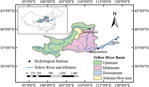
Three hydrological stations, namely Toudaoguai, Huayuankou, and Lijin, are selected to verify the VMD-LSTM-PSO model, which represent different climatic regions and hydrological conditions of the Yellow River. Toudaoguai Station controls the wide river valley in the upper reaches and is located in the transitional zone, where the channel changes from meandering to straight. Huayuankou Station controls approximately 97% of the total Yellow River Basin area (Tang et al. 2013). Lijin Station is the final hydrological station on the Yellow River and controls the flow of the river into the sea (Fig. 1).

The data for daily streamflow were derived from the Yellow River Conservancy Commission and are available for Toudaoguai, Huayuankou, and Lijin stations. All data were measured and quality controlled according to the Chinese national standard criteria. Detailed information regarding the streamflow series is listed in Table 1.

Table 1. Daily runoff series information at three stations on the Yellow River

Station	Area (km^2)	Dataset
		Training	Testing
Toudaoguai	36 7898	1 January 1954–31 December 2002	1 January 2003–31 December 2006
Huayuankou	73 0000	1 January 1957–31 December 2008	1 January 2009–31 December 2012
Lijin	75 1900	1 January 1950–31 December 2010	1 January 2011–31 December 2014

3 Methodology

3.1 Variational mode decomposition

3.1.1 Theory of variational mode decomposition

Dragomiretskiy and Zosso (2014) proposed an adaptive, nonrecursive signal decomposition method named variational modal decomposition. The goal of VMD is to decompose a real-valued input signal f into a discrete number of IMFs, $u_k{\mathrm{u}}_{\mathrm{k}}$, that are band limited. IMFs are amplitude-modulated/frequency-modulated (AM/FM) signals, which are expressed as follows:

(1) $u_k\left(t\right)=A_k\left(t\right)cos\left({\varphi }_k\left(t\right)\right)$(1)

where the phase ${\varphi }_k\left(t\right)$ is a nondecreasing function, ${\varphi }_k^{\prime }\left(t\right)\ge 0$, the envelope is nonnegative $A_k\left(t\right)\ge 0$, and, importantly, both the envelope $A_k\left(t\right)$ and the instantaneous frequency ${\omega }_k\left(t\right)={\varphi }_k^{\prime }\left(t\right)$ vary much more slowly than the phase ${\varphi }_k\left(t\right)$.

To acquire the bandwidth of each mode $u_k$, the constrained variational optimization problem is expressed as follows:

(2) $\underset{u_k{w}_k}{min}\left\{\sum _{k=1}^K{\mathrm{\partial }}_t\left[\left(\delta \left(t\right)+\frac{j}{\pi t}\right)\otimes u_k\left(t\right)\right]{e^{-j{w}_{k}t}}_2^2\right\}s.t\sum _{k=1}^K{u}_k=f\left(t\right)$(2)

where ${\omega }_k$ is the centre frequency of the corresponding kth mode of the signal, k is the number of modes, and $\delta \left(t\right)$ is the Dirac function. In addition, the expression $\left(\delta \left(t\right)+\frac{j}{\pi t}\right)\ast u_k\left(t\right)$ is the Hilbert transform of $u_k\left(t\right)$, which can transform$u_k\left(t\right)$ into the analytical signal to form a one-sided frequency spectrum with only positive frequencies. In this manner, using the index terms $e^{-j{\omega }_{k}t}$, the spectrum of each mode can be shifted to a baseband.

Two parameters, the quadratic penalty factor α and Lagrange multipliers λ, are both considered to transform the above optimization problem into an unconstrained optimization problem. The augmented Lagrange function is given as follows:

(3) $\mathrm{L}\left(u_k,w_k,\lambda \right)=\alpha \sum _{k=1}^K{\mathrm{\partial }}_t\left[\left(\delta \left(t\right)+\frac{j}{\pi t}\right)\otimes u_k\left(t\right)\right]{e^{-j{w}_{k}t}}_2^2+f\left(t\right)-\sum _{k=1}^K{u}_k{\left(t\right)}_2^2$(3)

where $||f\left(t\right)-{\sum }_{k=1}^K{u}_k\left(t\right)|{|}_2^2$ is a quadratic penalty term to accelerate the convergence velocity.

According to the optimization technique known as alternate direction method of multipliers (ADMM), $u_k$ and ${\omega }_k$ can be updated in two directions to complete the analysis of the VMD. Therefore, the updated equations are given as follows:

(4) ${\hat{u}}_k^{n+1}=\frac{\hat{f}\left(\omega \right)-{\sum }_{i\ne k}{\hat{u}}_i\left(\omega \right)+\frac{\hat{\lambda }\left(\omega \right)}{2}}{1+2\alpha {\left(\omega -{\omega }_k\right)}^2}$(4)

(5) ${\omega }_k^{n+1}=\frac{{\int }_0^{\mathrm{\infty }}\omega {\left|{\hat{u}}_k\left(\omega \right)\right|}^{2}d\omega }{{\int }_0^{\mathrm{\infty }}{\left|{\hat{u}}_k\left(\omega \right)\right|}^{2}d\omega }$(5)

(6) ${\omega }_k^{n+1}=\frac{{\int }_0^{\mathrm{\infty }}\omega {\left|{\hat{u}}_k\left(\omega \right)\right|}^{2}d\omega }{{\int }_0^{\mathrm{\infty }}{\left|{\hat{u}}_k\left(\omega \right)\right|}^{2}d\omega }$(6)

where n is the number of iterations, τ is the iterative factor, and ${\hat{u}}_k\left(\omega \right)$, ${\hat{u}}_k^{n+1}$, $\hat{f}\left(\omega \right)$, and $\hat{\lambda }\left(\omega \right)$ represent the Fourier transform of $u_k\left(\omega \right)$, $u_k^{n+1}$, $\mathrm{H}\mathrm{D}\mathrm{S}\mathrm{P}\mathrm{\_}\mathrm{A}\mathrm{\_}1938879$, and $\lambda \left(\omega \right)$, respectively.

3.1.2 Determination of decomposition level

To adaptively determine the number of decomposition layers k, the permutation entropy optimization algorithm (PEO; Bandt and Pompe 2002, Stosic et al. 2017) is employed, which can adaptively determine the number of decomposition layers k according to the characteristics of the signal to be decomposed. The principle of the algorithm is to calculate the permutation entropy of the inherent modal function of each layer obtained from the original signal decomposition. Due to the randomness of the abnormal component, the permutation entropy value is much larger than the normal component. Therefore, after setting the threshold H_p of the permutation entropy, we can judge whether the permutation entropy of each layer of IMF in the decomposition result is larger than the threshold H_p, so as to determine whether there is an abnormal component in the decomposition result, where the threshold H_p of permutation entropy is 0.6. The decomposition process of VMD method is shown in Fig. 2.

Figure 2. The variational mode decomposition (VMD) flow chart

The specific steps of the algorithm are as follows:

Step 1: Set the initial value of k as 2, and the threshold of permutation entropy as the empirical value of 0.6 (Wang et al. 2018).

Step 2: Decompose the original signal via the EMD algorithm to obtain k intrinsic modal functions IMF$i$(t) ($i$=1 ~ k).

Step 3: Calculate the permutation entropy Pei ($i$=1 ~ k) of each IMF in the decomposition result.

Step 4: Judge whether Pei is larger than the threshold of 0.6. If so, this indicates that the decomposition result has been overly decomposed, resulting in abnormal components. Then stop the cycle and execute step 5. If not, it means that no decomposition has occurred, and the number of decomposition layers of the original signal needs to be increased. Then let k = k + 1, return to step 2, and continue VMD decomposition of the original signal according to the updated k value.

Step 5: Let k = k − 1, output the optimal k, and, finally, decompose the sequence by using the VMD algorithm to obtain k IMFs.

3.2 Long short-term memory network

The LSTM structure is a special RNN designed to overcome the weakness of long-term dependence of traditional RNN learning (Hochreiter and Schmidhuber 1997, Zhang et al. 2018c, Le et al. 2019). All RNNs connect repeating neural network modules in a chain. LSTM differs from the original RNN in that this repeating module has different internal structures (Kratzert et al. 2018, Zhang et al. 2018b, Kao et al. 2020). This repeating module has only a simple tanh layer in the original RNN, as shown in Fig. 3(a). In the LSTM network, this module involves the four neural network layers that interact in a special way.

Figure 3. Schematic diagram of network module: (a) Recurrent neural network (RNN), (b) Long short-term memory (LSTM)

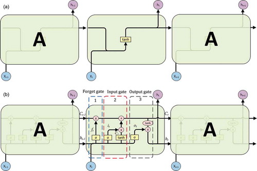
In the original RNN, there is only one internal state, $h_t$, which is very sensitive to short-term inputs. In LSTM, a new state C (i.e. cell state) is used to save the long-term state, so that the LSTM has the ability to handle long-term dependencies. As can be seen from Fig. 3(b), the LSTM has three inputs and two outputs at time t. The inputs are the output value $h_{t-1}$ of the LSTM at the last moment, the input value $x_t$ of the current moment, and the unit state $C_{t-1}$ at the previous moment. The outputs are the unit state $C_t$ and the output value $h_t$ of LSTM at the current moment.

The key to LSTM is control of the long-term state C. To this end, the neural network module of LSTM uses a gate structure, including a forget gate, input gate, and output gate, as shown in Fig. 3. Among them, the forget gate, the input gate, and the output gate are used to control the storage of the long-term state C, the information input by the current state into the long-term state C and the output of the long-term state C in the current LSTM module, respectively. The structure of each door is specifically introduced as follows:

1. Forget gate

The forget gate reads $h_{t-1}$ and $x_t$, and outputs a value between 0 and 1 to determine the proportion of information retention in the previous unit state$C_{t-1}$. 1 means “completely reserved,” and 0 means “completely discarded.” The equation is as follows:

(7) $f_t=\sigma \left(W_f\ast \left[h_{t-1},x_t\right]+b_f\right)$(7)

• (2) Input gate

Input gate $i_t$ determines the information used to update the final unit state $C_t$ of the current time step in the current input unit state ${\tilde{C}}_t$. Among them, ${\tilde{C}}_t$ is the unit state information under the current input calculated from the output $h_{t-1}$ at the previous time and the input $x_t$ at the current time. The value range is (−1, 1), and the range of $i_t$ is (0,1). The equation is as follows:

(8) $i_t=\sigma \left(W_i\ast \left[h_{t-1},x_t\right]+b_i\right)$(8)

(9) $\widetilde{C_t}=\mathrm{t}\mathrm{a}\mathrm{n}\mathrm{h}\left(W_{\tilde{c}}\ast \left[h_{t-1},x_t\right]+b_{\tilde{c}}\right)$(9)

The cell state $C_t$ at the current moment can be calculated from the forget gate and the input gate. The equation is as follows:

(10) $C_t=f_t\ast C_{t-1}+i_t\ast \widetilde{C_t}$(10)

(3) Output gate

The output gate $o_t$ determines the information in $C_t$ that is used to output $h_t$ at the current moment, where $C_t$is processed by tanh to get a value between −1 and 1. The equations of $o_t$ and $h_t$ are as follows:

(11) $o_t=\sigma \left(W_o\ast \left[h_{t-1},x_t\right]+b_o\right)$(11)

(12) $h_t=o_t\ast \mathrm{t}\mathrm{a}\mathrm{n}\mathrm{h}\left(C_t\right)$(12)

In the above equation, W is the weight matrix of each gate, $\sigma$ is the sigmoid function, and b is the offset term of each gate. “*” in the above equation represents a vector product.

3.3 PSO algorithm

PSO is a stochastic evolution technique used to solve global optimization problems, which is inspired by natural grouping behaviours, such as bird aggregation and fish learning (Kennedy and Eberhart 1995, Feng et al. 2019). PSO and its variants have been successfully employed in hydrological applications based on ANN (Chau 2006, Tapoglou et al. 2014, Feng et al. 2020). On the strength of the search strategy of the particle population, each random particle is identified by its position and speed in the process of search. The current particles are evaluated according to the fitness, and the local optimal information and global optimal information in the path are memorised. Based on the exchange of all the particle information, the better particles are selected to enter the next iteration and finally converge to the global optimal solution. Details on the steps of PSO can be found in the literature (Wang et al. 2013, Taormina and Chau 2015, Niu et al. 2018, Feng et al. 2020).

Moreover, CEEMD and WT methods are also involved and used in this paper, details of which can be found in the following sources (Kim and Valdés 2003, Küçük and Ağirali˙Oğlu 2006, Wu and Huang 2009, Adamowski and Sun 2010, Yeh et al. 2010, Torres et al. 2011, Singh 2012).

3.4 Streamflow forecasting based on VMD-LSTM-PSO model

For a runoff series, the establishment of the model mainly includes three steps: (1) decomposition stage; (2) network parameter optimization and network training stage; (3) prediction stage. In the first step, the original runoff series is decomposed into k IMFs using an improved VMD algorithm, transforming the original nonlinear hydrological series into more stable series. Then, each IMF is operated in the following steps. In the second step, the PSO algorithm is employed to optimise multiple parameters of the LSTM network, mainly including the number of hidden layer nodes and the learning rate of LSTM; also, the LSTM network is established using the optimised parameters, and the corresponding subsequence data is used to train the network. In the third step, the trained network is applied to predict the subsequence. Finally, the result can be obtained by summing the prediction results of each IMF component. The overall framework of the VMD-LSTM-PSO model is shown in Fig. 4.

Figure 4. Sketch map of the hybrid method for daily streamflow prediction

3.5 Model performance evaluation

The forecasting performance is evaluated using the following four statistical indices: Nash-Sutcliffe efficiency coefficient (NSE), the root mean of squared errors (RMSE), correlation coefficient (R), and Kolmogorov-Smirnov (K-S) distance. The NSE is a normalised statistic that determines the relative magnitude of the residual variance compared to the measured data variance (Nash and Sutcliffe 1970). NSE values range from negative infinity to 1, with 1 indicating an exact match between simulated and observed values. K-S is a nonparametric hypothesis test, which is used in statistics to test whether two samples obey the same distribution. The K-S statistic is the maximum difference of the empirical distribution function of the two samples, and ${\bar{D}}_n$ is the critical value of the K-S statistic with 95% confidence. If the value of the K-S statistic obtained from the sample is less than ${\bar{D}}_n$, then we accept the original hypothesis; otherwise, we reject the original hypothesis. The definitions of these statistics are given as follows:

(13) $NSE=1-\frac{{\sum }_{i=1}^n{\left(O_i-P_i\right)}^2}{{\sum }_{i=1}^n{\left(O_i-\bar{O}\right)}^2}$(13)

(14) $R=\frac{{\sum }_{i=1}^n\left(O_i-\bar{O}\right)\left(P_i-\bar{P}\right)}{\sqrt{{\sum }_{i=1}^n{\left(O_i-\bar{O}\right)}^2{\sum }_{i=1}^n{\left(P_i-\bar{P}\right)}^2}}$(14)

(15) $RMSE=\sqrt{\frac{{\sum }_{i=1}^n{\left(O_i-P_i\right)}^2}{n}}$(15)

(16) ${\bar{D}}_n=1.36\sqrt{\frac{1}{n_x}+\frac{1}{n_y}}$(16)

where $O_i$ is the measured value, $P_i$ is the simulated value, $\bar{O}$ is the measured average, $\bar{P}$ is the average of the simulated value, n is the number of measured values, ${\bar{D}}_n$ is the critical value of the K-S statistic with 95% confidence, and $n_x$ and $n_y$ are the sample sises of two sample sequences.

4 Results and discussion

The improved VMD decomposition has self-adaptability and strong noise reduction performance. It can decompose a complex time series composed of different frequency components into multiple subsequences with inherent modal functions. Based on the decomposed subsequences, the LSTM-PSO prediction model is established. The sum of the prediction results of each subsequence is the prediction result of the original sequence. In the following, the daily runoff sequences of Toudaoguai Station from 1 January 1954 to 31 December 2006, Huayuankou Station from 1 January 1957 to 31 December 2012, and Lijin Station from 1 January 1950 to 31 December 2014 are used as research objects to establish VMD-LSTM-PSO prediction models.

4.1 Decomposition results using VMD

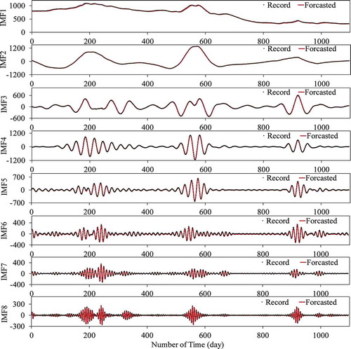
A problem of LSTM and other linear and nonlinear forecast models is that they are not able to handle nonstationary data. To cope with the nonstationary problem of the streamflow, the improved VMD method described in Section 3.1 is used to decompose the daily runoff series of Toudaoguai, Huayuankou and Lijin stations, and k components can be adaptively obtained. The number of IMFs obtained from the VMD decomposition is shown in Table 2. Among them, taking Lijin Station as an example, the decomposition results are shown in Fig. 5. The original series is decomposed into eight IMF components in Fig. 5 with similar frequency using the VMD technique, which shows the nonlinear, trend, periodicity and other characteristics of the original hydrological series. Accordingly, the prediction effectiveness of each component is improved gradually, leading to an increase in the NSE and R values, and a decrease in the RMSE value. The VMD method can effectively remove the nonstationary characteristics associated with the original series and generate cleaner input for the LSTM model, which contributes to a significant improvement in the forecasting accuracy.

Table 2. Statistics of variational mode decomposition (VMD) results of daily runoff at the three stations of the Yellow River

Station	Time series	No. of IMFs
Toudaoguai	1 January 1954–31 December 2006	8
Huayuankou	1 January 1957–31 December 2012	6
Lijin	1 January 1950–31 December 2014	8

Figure 5. Prediction results of each component of the variational mode decomposition (VMD) at Lijin Station

4.2 Model building and inputs

For each IMF, LSTM is applied to establish the prediction model. Critical parameters such as the numbers of inputs, hidden layers, hidden nodes, and learning rate are prerequisites for the prediction performance of the LSTM model. Therefore, PSO is utilised to automatically calibrate the parameters of the LSTM model. The LSTM-PSO not only inherits the advantages of the LSTM, but also utilises the superiority of the PSO for solving optimization problems, where the process of population evolution can interact with the LSTM in the training process, and optimise the number of hidden nodes and the learning rate (α) of the LSTM model (HN). The number of nodes in the input layer is equal to the number of input variables, while the number of nodes in the output layer is 1. The number of hidden layers is 2.

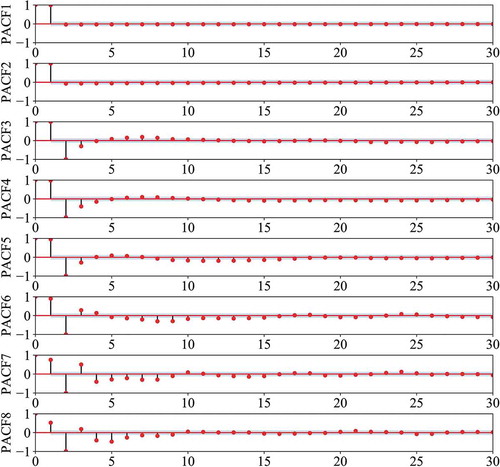
In addition, to determine the influence of suitable time lag runoff on the current t time interval runoff, the partial autocorrelation function (PACF) was employed to determine the input step sise of the LSTM model. The input variables are determined by analysing the resulting partial autocorrelation diagram – that is, the plots of PACF corresponding to the lag length. Specifically, assuming that the output variable is x_i, on the condition that the PACF at lag k is out of the 95% confidence interval, then x_i-k is one of the input variables (Huang et al. 2014). Figure 6 shows the PACF of each IMF decomposed by VMD at Lijin Station. The input step recognition of each station is shown in Table 3.

Table 3. Input step optimization for each station

Station	Decomposed IMFs	No. of inputs	Input variables	Output
Toudaoguai	IMF1	4	x1 (t-1)(t-2)(t-3)(t-4)	x1(t)
	IMF2	4	x2 (t-1)(t-2)(t-3)(t-4)	x2(t)
	IMF3	4	x3 (t-1)(t-2)(t-3)(t-4)	x3(t)
	IMF4	3	x3 (t-1)(t-2)(t-3)	x3(t)
	IMF5	2	x5 (t-1)(t-2)	x5(t)
	IMF6	1	x6 (t-1)	x6(t)
	IMF7	1	x7 (t-1)	x7(t)
	IMF8	1	x8 (t-1)	x8(t)
Huayuankou	IMF1	1	x1 (t-1)	x1(t)
	IMF2	4	x2 (t-1)(t-2)(t-3)(t-4)	x2(t)
	IMF3	5	x3 (t-1)(t-2)(t-3)(t-4)(t-5)	x3(t)
	IMF4	3	x4 (t-1)(t-2)(t-3)	x3(t)
	IMF5	7	x5 (t-1)(t-2)(t-3)(t-4)(t-5) (t-6)(t-7)	x5(t)
	IMF6	9	x6 (t-1)(t-2)(t-3)(t-4)(t-5) (t-6)(t-7)(t-8)(t-9)	x6(t)
Lijin	IMF1	1	x1 (t-1)	x1(t)
	IMF2	1	x2 (t-1)	x2(t)
	IMF3	3	x3 (t-1)(t-2)(t-3)	x3(t)
	IMF4	4	x4 (t-1)(t-2)(t-3)(t-4)	x3(t)
	IMF5	3	x5 (t-1)(t-2)(t-3)	x5(t)
	IMF6	4	x6 (t-1)(t-2)(t-3)(t-4)	x6(t)
	IMF7	8	x7 (t-1)(t-2)(t-3)(t-4)(t-5) (t-6)(t-7)(t-8)	x7(t)
	IMF8	8	x8 (t-1)(t-2)(t-3)(t-4)(t-5) (t-6)(t-7)(t-8)	x8(t)

Figure 6. The partial autocorrelation function (PACF) of each intrinsic mode functions (IMF) decomposed by VMD at Lijin Station

4.3 Forecasting results

This model is applied to forecast the streamflow of the three stations in the Yellow River. The input step sise of the LSTM model is determined according to PACF, and the LSTM-PSO prediction model of each IMF is constructed based on VMD decomposition. The ensemble prediction results were obtained by summing the prediction subresults of the modelled IMFs from the daily runoff data during the period. The NSE, RMSE, R and K-S distance are used to evaluate the accuracy of the prediction model. Daily runoff data are divided into two parts: a calibration dataset and a validation dataset. Data for the last 3 years are used as the test period, and the remainder is used for training. The prediction results of each station are summarised in Table 4. Figure 6 shows the prediction results of each component of VMD at Lijin Station.

Table 4. Evaluation of variational mode decomposition coupled long short-term memory and particle swarm optimization (VMD-LSTM-PSO) model prediction results at each station

Station	Evaluation index	IMF1	IMF2	IMF3	IMF4	IMF5	IMF6	IMF7	IMF8	Ensemble result
Toudaoguai	NSE	0.9980	0.9989	0.9986	0.9964	0.9908	0.9892	0.9949	0.9944	0.9857
	RMSE (m^3 s^−1)	3.503	5.940	4.678	5.394	6.291	5.089	2.466	1.788	37.02
	R	0.9997	0.9990	0.9997	0.9992	0.9970	0.9954	0.9981	0.9973	0.9931
Huayuankou	NSE	0.9992	0.9996	0.9978	0.9779	0.9411	0.9746	/	/	0.9760
	RMSE (m^3 s^−1)	9.495	6.834	16.16	20.72	19.69	9.742	/	/	115.5
	R	0.9999	0.9998	0.9990	0.9951	0.9719	0.9933	/	/	0.9900
Lijin	NSE	0.9981	0.9999	0.9981	0.9987	0.9969	0.9754	0.9944	0.9933	0.9942
	RMSE (m^3 s^−1)	11.11	5.219	7.782	9.637	7.276	11.56	4.097	3.937	56.38
	R	0.9995	1	0.9997	0.9995	0.9994	0.9965	0.9973	0.9981	0.9972

It can be seen intuitively from Fig. 6 that the decomposed IMF component prediction results of VMD-LSTM-PSO have a good fit with the recorded values. The statistical results in Table 4 also provide detailed and powerful data support for the above conclusions. Through the calculation and comparison at three sites, we can conclude that the VMD method can transform the nonlinear hydrological data into several relatively stationary time series, which will be helpful to enhance the performance of forecasting models (Fig. 5), and the VMD-LSTM-PSO model can attain acceptably accurate predictions for daily runoff simulations (Table 4).

4.4 Comparative analysis

To further test the feasibility and superiority of the VMD-LSTM-PSO hybrid model, comparisons of four kinds of daily-scale runoff prediction models – VMD-LSTM-PSO, CEEMD-LSTM-PSO, WT-LSTM-PSO, LSTM-PSO – are carried out in this experiment. The comparison between VMD-LSTM-PSO and LSTM-PSO is designed to prove the positive effects of decomposition techniques, and comparisons of VMD-LSTM-PSO, CEEMD-LSTM-PSO, and WT-LSTM-PSO are performed to demonstrate the advantages of the VMD decomposition technique among the three prevailing decomposition methods. On the basis of EMD decomposition, the CEEMD method adds two opposite white noise signal pairs to the analysis signal to achieve a decomposition effect equivalent to EEMD, while reducing the reconstruction error caused by white noise (Yeh et al. 2010).

Wavelet analysis is a time-frequency multiresolution analysis method that can fully extract the different frequency components contained in a sequence (Wang et al. 2007). In this study, orthogonal Db4 wavelets were used to obtain low-frequency components C3 and high-frequency components D3, D2, and D1. We selected the data from the last 3 years for verification, and used the rest for training, respectively evaluating the prediction effectiveness of VMD-LSTM-PSO, CEEMD-LSTM-PSO, WT-LSTM-PSO, and LSTM-PSO. Tables 5–8 show the prediction performance evaluation indices of the different models, and Table 8 shows whether the predicted samples of each prediction model conform to the same distribution as the measured samples. Figures 7 and 8 show the observed and simulated data obtained by different methods. To better display the results, a part of the whole prediction series is intercepted and magnified to better show the fitting degree of the peaks and valleys of the prediction sequence. The whole prediction sequence and the intercepted partial prediction sequence correspond to the small graph and the magnified image, respectively.

Table 5. Prediction performance evaluation indices of different models at Toudaoguai Station

Model	VMD-LSTM-PSO			CEEMD-LSTM-PSO			WT-LSTM-PSO			LSTM-PSO
	NSE	RMSE (m^3 s^−1)	R	NSE	RMSE (m^3 s^−1)	R	NSE	RMSE (m^3 s^−1)	R	NSE	RMSE (m^3 s^−1)	R
IMF1	0.9980	3.503	0.9997	−0.0530	40.32	0.5228	0.9938	23.36	0.9970	/	/	/
IMF2	0.9989	5.940	0.9990	0.9470	14.13	0.9858	−0.0212	27.16	0.6363	/	/	/
IMF3	0.9986	4.678	0.9997	0.9812	12.49	0.9965	0.5855	29.67	0.8593	/	/	/
IMF4	0.9964	5.394	0.9992	0.9849	13.39	0.9990	0.8758	26.05	0.9371	/	/	/
IMF5	0.9908	6.291	0.9970	0.9995	3.318	0.9999	/	/	/	/	/	/
IMF6	0.9892	5.089	0.9954	0.9844	13.60	0.9938	/	/	/	/	/	/
IMF7	0.9949	2.466	0.9981	0.9941	3.493	0.9992	/	/	/	/	/	/
IMF8	0.9944	1.788	0.9973	0.9982	1.526	0.9995	/	/	/	/	/	/
IMF9	/	/	/	0.9999	0.3360	0.9999	/	/	/	/	/	/
Ensemble result	0.9857	37.02	0.9931	0.9849	38.01	0.9925	0.9812	42.48	0.9914	0.9383	76.91	0.9715

Table 6. Prediction performance evaluation indices of different models at Huayuankou Station

Model	VMD-LSTM-PSO			CEEMD-LSTM-PSO			WT-LSTM-PSO			LSTM-PSO
	NSE	RMSE (m^3s^−1)	R	NSE	RMSE (m^3s^−1)	R	NSE	RMSE (m^3s^−1)	R	NSE	RMSE (m^3s^−1)	R
IMF1	0.9992	9.495	0.9999	−0.1323	110.6	−0.1323	0.9941	54.58	0.9971	/	/	/
IMF2	0.9996	6.834	0.9998	0.7473	72.84	0.8807	−0.0642	88.42	−0.3133	/	/	/
IMF3	0.9978	16.16	0.9990	0.9833	37.41	0.9950	0.6803	63.24	0.8506	/	/	/
IMF4	0.9779	20.72	0.9951	0.9935	19.31	0.9993	0.7690	90.64	0.8990	/	/	/
IMF5	0.9411	19.69	0.9719	0.9997	4.542	0.9999	/	/	/	/	/	/
IMF6	0.9746	9.742	0.9933	0.9970	26.04	0.9995	/	/	/	/	/	/
Ensemble result	0.9760	115.5	0.9900	0.9633	143.0	0.9832	0.9656	138.4	0.9828	0.9204	210.5	0.9598

Table 7. Prediction performance evaluation indices of different models at Lijin Station

Model	VMD-LSTM-PSO			CEEMD-LSTM-PSO			WT-LSTM-PSO			LSTM-PSO
	NSE	RMSE (m^3s^−1)	R	NSE	RMSE (m^3s^−1)	R	NSE	RMSE (m^3s^−1)	R	NSE	RMSE (m^3s^−1)	R
IMF1	0.9981	11.11	0.9995	−1.017	60.18	0.4032	0.9971	38.96	0.9992	/	/	/
IMF2	0.9999	5.219	1.0000	−0.8157	20.39	0.5527	−0.2671	48.51	0.8322	/	/	/
IMF3	0.9981	7.782	0.9997	0.3323	44.88	0.6637	0.7444	42.67	0.8915	/	/	/
IMF4	0.9987	9.637	0.9995	0.9187	21.11	0.9603	0.9301	36.58	0.9645	/	/	/
IMF5	0.9969	7.276	0.9994	0.9941	11.66	0.9985	/	/	/	/	/	/
IMF6	0.9754	11.56	0.9965	0.9646	39.14	0.9973	/	/	/	/	/	/
IMF7	0.9944	4.097	0.9973	0.9855	15.95	0.9994	/	/	/	/	/	/
IMF8	0.9933	3.937	0.9981	0.9993	5.040	1.0000	/	/	/	/	/	/
IMF9	/	/	/	0.9992	7.072	0.9999	/	/	/	/	/	/
IMF10	/	/	/	0.9963	19.73	0.9989	/	/	/	/	/	/
IMF11	/	/	/	0.9960	6.905	0.9998	/	/	/	/	/	/
IMF12	/	/	/	0.9998	2.045	1.0000	/	/	/	/	/	/
IMF13	/	/	/	0.9969	1.008	0.9999	/	/	/	/	/	/
IMF14	/	/	/	0.9065	1.022	1.0000	/	/	/	/	/	/
IMF15	/	/	/	0.8642	1.287	1.0000	/	/	/	/	/	/
IMF16	/	/	/	−0.8294	1.087	1.0000	/	/	/	/	/	/
Ensemble result	0.9942	56.38	0.9972	0.9909	70.41	0.9964	0.9820	99.11	0.9963	0.9676	132.9	0.9850

Table 8. Kolmogorov - Smirnov (K-S) distance of different prediction models at each hydrological stations

Model	Toudaoguai Station	Huanyuankou Station	Lijin Station	95% confidence degree
VMD -LSTM-PSO	0.0237	0.0274	0.0465	0.0580
WT -LSTM-PSO	0.0401	0.0292	0.1460	0.0580
CEEMD -LSTM-PSO	0.0420	0.0502	0.0684	0.0580
LSTM-PSO	0.0776	0.0566	0.0484	0.0580

Figure 7. Comparison of the prediction results from different models at (a) Toudaoguai Station, (b) Huayuankou Station and (c) Lijin Station

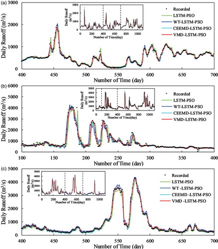
Figure 8. Comparison of the prediction results at (a) Toudaoguai Station, (b) Huayuankou Station and (c) Lijin Station

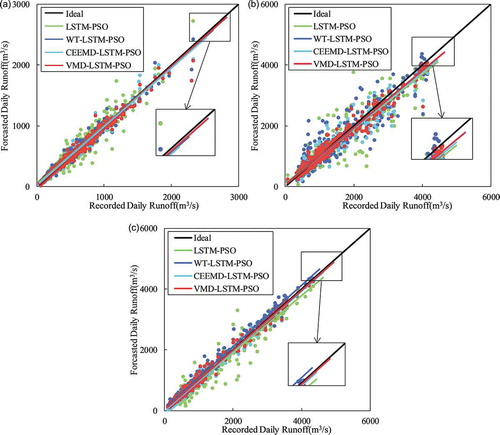
The simulations demonstrate that there are distinct differences between the VMD, CEEMD, and WT methods, indicating the importance of decomposition tools in forecasting models. The VMD-LSTM-PSO model always has the best performance with respect to four indices as compared with other methods (Tables 5–8), and the trend line of the VMD-LSTM-PSO model in Fig. 8 (the red fitting line) is closest to the ideal trend line (the black fitting line), which reaffirms the superiority and prediction accuracy of the hybrid model. Taking Lijin Station as an example, for the daily runoff dataset, the model in the testing period yielded an NSE value of approximately 0.994 (VMD-LSTM-PSO) vs. 0.99 (CEEMD-LSTM-PSO), 0.982 (WT-LSTM-PSO) and 0.968 (LSTM-PSO), whereas the RMSE is 56.375 m³ s⁻¹ (VMD-LSTM-PSO) vs. 70.405 m³ s⁻¹ (CEEMD-LSTM-PSO), 99.113 m³ s⁻¹ (WT-LSTM-PSO) and 132.909 m³ s⁻¹ (LSTM-PSO). Another measure of the tested model accuracy, the correlation coefficient, R, is found to be approximately 0.997 (VMD-LSTM-PSO) vs. 0.996 (CEEMD-LSTM-PSO), 0.996 (WT-LSTM-PSO) and 0.985 (LSTM-PSO). The prediction accuracy is ranked from high to low as VMD-LSTM-PSO > CEEMD-LSTM-PSO > WT-LSTM-PSO > LSTM-PSO. As to the K-S distance analysis, the predicted samples of VMD-LSTM-PSO and LSTM-PSO obey the same distribution as the measured samples, and the distribution similarity rate of the VMD-LSTM-PSO method is higher, which indicates the model proposed in this paper has stronger generalizability. The analysis of the results of the VMD-LSTM-PSO and LSTM-PSO methods shows that the NSE coefficients of LSTM-PSO are all greater than 0.9, for the three typical hydrological stations in the Yellow River basin, which confirms the feasibility of applying LSTM to runoff forecasting in the Yellow River basin. From the analysis of the four evaluation indices, the accuracy of the models is in the order VMD-LSTM-PSO > LSTM-PSO, which indicates that no additional data error is added in the hybrid calculation, and the proposed VMD-LSTM-PSO hybrid model is reliable and exhibits higher accuracy in the daily runoff prediction.

Analysis of Figs 7 and 8 shows that VMD-LSTM-PSO prediction values have a very high degree of fit with the recorded values, and the peak and valley values have a good prediction effectiveness. However, by observing the prediction results of the 550th day of Lijin Station, it can be seen that the predicted values of CEEMD-LSTM-PSO and WT-LSTM-PSO are overfitted with the measured values, and the fitting effect of the peak and valley values is not as good as that of the VMD-LSTM-PSO model. According to Table 5, VMD has eight IMF components and the prediction effectiveness is good; CEEMD has 16 IMF components among which IMF1, IMF2, IMF3, and IMF16 do not meet the accuracy requirements; WT decomposition has four IMF components of which both IMF2 and IMF3 are high-frequency components whose prediction effectiveness is poor.

It can be concluded that there are many pseudo components in CEEMD, which not only reduces the prediction accuracy of the LSTM model but also increases the running time of the model. Compared to EEMD decomposition, CEEMD suppresses the modal confusion problem to a certain extent, but there are many pseudo components. Some information, such as the decomposition level and mother wavelets, should be predetermined in WT. Inappropriate wavelet bases and decomposition level will result in a poor decomposition effect of high-frequency components. In this study, orthogonal Db4 wavelets were used to obtain low-frequency components C3 and high-frequency components D3, D2, and D1. In fact, compared with the WT technique and CEEMD technique, the VMD technique has the advantages of effectively reducing pseudo components and avoiding modal aliasing, and has better noise robustness. Consequently, VMD-LSTM-PSO has better prediction performance than other hybrid models. In sum, the integration of data decomposition, intelligent algorithm and parameter optimization into the prediction model can provide accurate daily runoff forecasting results for operators, which can be employed as valuable technical references for relevant studies in the field of hydrological forecasting.

5 Conclusions

For the sake of resolving the nonlinear and nonstationarity challenges faced by conventional runoff forecasting models and improving daily runoff prediction accuracy, a hybrid model named VMD-LSTM-PSO was proposed to accurately perform daily runoff forecasting. Furthermore, to demonstrate the applicability of the hybrid model in daily runoff forecasting, the prediction results of the VMD-LSTM-PSO model were compared with LSTM-PSO, CEEMD-LSTM-PSO, and EEMD-LSTM-PSO to evaluate its prediction effectiveness.

Generally speaking, the VMD-LSTM-PSO model proposed in this paper can attain high forecasting accuracy of daily nonstationary runoff series. Compared with other conventional runoff prediction models, the main features of the proposed model can be summarised as follows:

1. The VMD method can effectively separate the internal characteristics of the original daily runoff to accurately describe the nonstationarity of hydrological sequences, and simultaneously has the advantages of effectively reducing pseudo-components and avoiding modal aliasing and better noise robustness.

2. LSTM-PSO can capture the long-term correlation of time series and has a strong nonlinear predictive capability to improve the reliability of daily runoff forecasting.

3. The VMD-LSTM-PSO model proposed in this paper outperforms all other comparison models for three typical hydrological stations in the Yellow River basin, which shows that the method has universal adaptability and can reflect the runoff characteristics of different regions. It is a promising alternative for improving the forecasting results of complex nonstationary daily runoff time series prediction.

It is worth noting that although the advantages and feasibility of the proposed hybrid model have been verified by actual data, there are still several potential problems and research directions to investigate. First, the proposed model needs to build an LSTM model for each sequence decomposed separately, and it needs to use the PSO algorithm to calibrate parameters, so the running time is long. To better capture the long-term correlation of the sequence and improve the prediction accuracy, there are certain requirements for the length of the data sequence. Second, the VMD-LSTM-PSO model proposed in this paper goes a long way in explaining the nonstationary characteristics of runoff series, and can be extended to other fields, such as the prediction of sediment concentration and power load, for further study of its universality. Third, the WT decomposition method is related to wavelet base and decomposition layer number. Future studies could try different decomposition layer numbers and wavelet bases to explore the possibility and accuracy of WT decomposition applications in runoff prediction.

Acknowledgements

The authors wish to acknowledge the assistance of all editors and reviewers.

Disclosure statement

No potential conflict of interest was reported by the authors.

Additional information

Funding

This study was supported by the National Key R&D Program of China (2018YFC1508403), the National Natural Science Foundation of China (51579173), the National Key R&D Program of China (2016YFC0401701) and the Science Fund for Creative Research Groups of the National Natural Science Foundation of China (51621092).

References

- Adamowski, J. and Sun, K., 2010. Development of a coupled wavelet transform and neural network method for flow forecasting of non-perennial rivers in semi-arid watersheds. Journal of Hydrology, 390 (1–2), 85–91. doi:10.1016/j.jhydrol.2010.06.033
- Ashrafi, M., et al., 2017. A fully-online neuro-fuzzy model for flow forecasting in basins with limited data. Journal of Hydrology, 545, 424–435. doi:10.1016/j.jhydrol.2016.11.057
- Bandt, C. and Pompe, B., 2002. Permutation entropy: a natural complexity measure for time series. Physical Review Letters, 88 (17), 174102. doi:10.1103/PhysRevLett.88.174102
- Chang, F.J., et al., 2015. Multi-step-ahead reservoir inflow forecasting by artificial intelligence Techniques. In: J.W. Tweedale, et al., ed. Knowledge-based information systems in practice. Cham: Springer International Publishing, 235–249.
- Chang, F.-J., et al., 2014. Real-time multi-step-ahead water level forecasting by recurrent neural networks for urban flood control. Journal of Hydrology, 517, 836–846. doi:10.1016/j.jhydrol.2014.06.013
- Chau, K.W., 2006. Particle swarm optimization training algorithm for ANNs in stage prediction of Shing Mun River. Journal of Hydrology, 329 (3–4), 363–367. doi:10.1016/j.jhydrol.2006.02.025
- Dragomiretskiy, K. and Zosso, D., 2014. Variational mode decomposition. IEEE Transactions on Signal Processing, 62 (3), 531–544. doi:10.1109/TSP.2013.2288675
- Fan, H., et al. 2020. Comparison of long short term memory networks and the hydrological model in runoff simulation. Water, 12 (1), 175. doi:10.3390/w12010175
- Feng, Z.-K., et al., 2019. Operation rule derivation of hydropower reservoir by k-means clustering method and extreme learning machine based on particle swarm optimization. Journal of Hydrology, 576, 229–238. doi:10.1016/j.jhydrol.2019.06.045
- Feng, Z.-K., et al., 2020. Monthly runoff time series prediction by variational mode decomposition and support vector machine based on quantum-behaved particle swarm optimization. Journal of Hydrology, 583, 124627. doi:10.1016/j.jhydrol.2020.124627
- Gao, S., et al., 2020. Short-term runoff prediction with GRU and LSTM networks without requiring time step optimization during sample generation. Journal of Hydrology, 589, 125188. doi:10.1016/j.jhydrol.2020.125188
- Ghaemi, A., et al., 2019. On the applicability of maximum overlap discrete wavelet transform integrated with MARS and M5 model tree for monthly pan evaporation prediction. Agricultural and Forest Meteorology, 278, 107647. doi:10.1016/j.agrformet.2019.107647
- He, X., et al.. 2019. Daily runoff forecasting using a hybrid model based on variational mode decomposition and deep neural networks. Water Resources Management, 33 (4), 1571–1590. doi:10.1007/s11269-019-2183-x
- He, Z., et al., 2014. A comparative study of artificial neural network, adaptive neuro fuzzy inference system and support vector machine for forecasting river flow in the semiarid mountain region. Journal of Hydrology, 509, 379–386. doi:10.1016/j.jhydrol.2013.11.054
- Hochreiter, S. and Schmidhuber, J., 1997. Long short-term memory. Neural Computation, 9 (8), 1735–1780. doi:10.1162/neco.1997.9.8.1735
- Huang, N.E., et al.. 1998. The empirical mode decomposition and the Hilbert spectrum for nonlinear and non-stationary time series analysis. Proceedings of the Royal Society of London. Series A: Mathematical, Physical and Engineering Sciences, 454 (1971), 903–995. doi:10.1098/rspa.1998.0193
- Huang, S., et al., 2014. Monthly streamflow prediction using modified EMD-based support vector machine. Journal of Hydrology, 511, 764–775. doi:10.1016/j.jhydrol.2014.01.062
- Humphrey, G.B., et al., 2016. A hybrid approach to monthly streamflow forecasting: integrating hydrological model outputs into a Bayesian artificial neural network. Journal of Hydrology, 540, 623–640. doi:10.1016/j.jhydrol.2016.06.026
- Hung, N.Q., et al.. 2009. An artificial neural network model for rainfall forecasting in Bangkok, Thailand. Hydrology and Earth System Sciences, 13 (8), 1413–1425. doi:10.5194/hess-13-1413-2009
- Kao, I.F., et al., 2020. Exploring a long short-term memory based encoder-decoder framework for multi-step-ahead flood forecasting. Journal of Hydrology, 583, 124631. doi:10.1016/j.jhydrol.2020.124631
- Kasiviswanathan, K.S., et al., 2013. Constructing prediction interval for artificial neural network rainfall runoff models based on ensemble simulations. Journal of Hydrology, 499, 275–288. doi:10.1016/j.jhydrol.2013.06.043
- Kennedy, J. and Eberhart, R., 1995. Particle swarm optimization. ed. In: Proceedings of ICNN’95 - international conference on neural networks, vol. 1944, Perth, Australia, 27 November–1 December 1995, 1942–1948.
- Kim, T.-W. and Valdés, J.B., 2003. Nonlinear model for drought forecasting based on a conjunction of wavelet transforms and neural networks. Journal Of Hydrologic Engineering, 8 (6), 319–328. doi:10.1061/(ASCE)1084-0699(2003)8:6(319)
- Kratzert, F., et al.. 2018. Rainfall–runoff modelling using Long Short-Term Memory (LSTM) networks. Hydrology and Earth System Sciences, 22 (11), 6005–6022. doi:10.5194/hess-22-6005-2018
- Küçük, M. and Ağirali˙Oğlu, N., 2006. Wavelet regression technique for streamflow prediction. Journal of Applied Statistics, 33 (9), 943–960. doi:10.1080/02664760600744298
- Le, X.-H., et al.. 2019. Application of Long Short-Term Memory (LSTM) neural network for flood forecasting. Water, 11 (7), 1387. doi:10.3390/w11071387
- Li, W., Kiaghadi, A., and Dawson, C., 2021. High temporal resolution rainfall–runoff modeling using long-short-term-memory (LSTM) networks. Neural Computing and Applications, 33 (4), 1261–1278. doi:10.1007/s00521-020-05010-6
- Li, X., et al.. 2020. Rainfall runoff prediction via a hybrid model of neighbourhood rough set with LSTM. International Journal of Embedded Systems, 13 (4), 405. doi:10.1504/IJES.2020.110654
- Maroufpoor, S., et al., 2019. Soil moisture simulation using hybrid artificial intelligent model: hybridization of adaptive neuro fuzzy inference system with grey wolf optimiser algorithm. Journal of Hydrology, 575, 544–556. doi:10.1016/j.jhydrol.2019.05.045
- Naganna, S.R., et al.. 2019. Dew point temperature estimation: application of artificial intelligence model integrated with nature-inspired optimization algorithms. Water, 11 (4), 742. doi:10.3390/w11040742
- Nash, J.E. and Sutcliffe, J.V., 1970. River flow forecasting through conceptual models part I - A discussion of principles. Journal of Hydrology, 10 (3), 282–290. doi:10.1016/0022-1694(70)90255-6
- Niu, W.-J., et al.. 2018. Forecasting daily runoff by extreme learning machine based on quantum-behaved particle swarm optimization. Journal Of Hydrologic Engineering, 23 (3), 04018002. doi:10.1061/(ASCE)HE.1943-5584.0001625
- Niu, W.-J., et al.. 2020. Short-term streamflow time series prediction model by machine learning tool based on data preprocessing technique and swarm intelligence algorithm. Hydrological Sciences Journal, 65 (15), 2590–2603. doi:10.1080/02626667.2020.1828889
- Qasem, N., et al.. 2019. Modeling monthly pan evaporation using wavelet support vector regression and wavelet artificial neural networks in arid and humid climates. Engineering Applications of Computational Fluid Mechanics, 13 (1), 177–187. doi:10.1080/19942060.2018.1564702
- Rezaie-Balf, M., et al., 2017. Wavelet coupled MARS and M5 model tree approaches for groundwater level forecasting. Journal of Hydrology, 553, 356–373. doi:10.1016/j.jhydrol.2017.08.006
- Rezaie-Balf, M., et al.. 2019b. Enhancing streamflow forecasting using the augmenting ensemble procedure coupled machine learning models: case study of Aswan High Dam. Hydrological Sciences Journal, 64 (13), 1629–1646. doi:10.1080/02626667.2019.1661417
- Shamshirband, S., et al., 2016. Estimating the diffuse solar radiation using a coupled support vector machine–wavelet transform model. Renewable and Sustainable Energy Reviews, 56, 428–435. doi:10.1016/j.rser.2015.11.055
- Shiau, J.-T. and Hsu, H.-T., 2016. Suitability of ANN-based daily streamflow extension models: a case study of Gaoping River Basin, Taiwan. Water Resources Management, 30 (4), 1499–1513. doi:10.1007/s11269-016-1235-8
- Shoaib, M., et al., 2016. A comparison between wavelet based static and dynamic neural network approaches for runoff prediction. Journal of Hydrology, 535, 211–225. doi:10.1016/j.jhydrol.2016.01.076
- Singh, R.M., 2012. Wavelet-ANN model for flood events. Advances in Intelligent and Soft Computing, 131, 165–175. doi:10.1007/978-81-322-0491-6_16
- Stosic, T., Stosic, B., and Singh, V.P., 2017. Optimizing streamflow monitoring networks using joint permutation entropy. Journal of Hydrology, 552, 306–312. doi:10.1016/j.jhydrol.2017.07.003
- Tan, Q.-F., et al., 2018. An adaptive middle and long-term runoff forecast model using EEMD-ANN hybrid approach. Journal of Hydrology, 567, 767–780. doi:10.1016/j.jhydrol.2018.01.015
- Tang, Y., et al.. 2013. Responses of natural runoff to recent climatic variations in the Yellow River basin, China. Hydrology and Earth System Sciences, 17 (11), 4471–4480. doi:10.5194/hess-17-4471-2013
- Taormina, R. and Chau, K.-W., 2015. Data-driven input variable selection for rainfall–runoff modeling using binary-coded particle swarm optimization and extreme learning machines. Journal of Hydrology, 529, 1617–1632. doi:10.1016/j.jhydrol.2015.08.022
- Tapoglou, E., et al.. 2014. Groundwater-level forecasting under climate change scenarios using an artificial neural network trained with particle swarm optimization. Hydrological Sciences Journal, 59 (6), 1225–1239. doi:10.1080/02626667.2013.838005
- Torres, M.E., et al., 2011. A complete ensemble empirical mode decomposition with adaptive noise. ed. In: 2011 IEEE International Conference on Acoustics, Speech and Signal Processing (ICASSP), Prague Congress Center, Prague, Czech Republic, 22–27 May 2011, 4144–4147.
- Wang, W.-C., et al.. 2013. Improved annual rainfall-runoff forecasting using PSO–SVM model based on EEMD. Journal of Hydroinformatics, 15 (4), 1377–1390. doi:10.2166/hydro.2013.134
- Wang, X., et al., 2007. Prediction model of daily runoff based on wavelet denoising. Journal of System Simulation, 15, 3605–3608. (in Chinese).
- Wang, Z., et al., 2018. Permutation entropy optimization improved variable modal decomposition algorithm to diagnose gearbox faults. Journal of Agricultural Engineering, 34 (23), 59–66. (in Chinese).
- Wu, Z. and Huang, N.E., 2009. Ensemble empirical mode decomposition: a noise-assisted data analysis method. Advances in Adaptive Data Analysis, 1 (1), 1–41. doi:10.1142/S1793536909000047
- Xie, T., et al., 2019. Hybrid forecasting model for non-stationary daily runoff series: a case study in the Han River Basin, China. Journal of Hydrology, 577, 123915.
- Yaseen, Z.M., et al., 2016. Stream-flow forecasting using extreme learning machines: a case study in a semi-arid region in Iraq. Journal of Hydrology, 542, 603–614. doi:10.1016/j.jhydrol.2016.09.035
- Yaseen, Z.M., et al.. 2018. Application of the hybrid artificial neural network coupled with rolling mechanism and grey model algorithms for streamflow forecasting over multiple time horizons. Water Resources Management, 32 (5), 1883–1899. doi:10.1007/s11269-018-1909-5
- Yaseen, Z.M., et al.. 2019a. A hybrid bat–swarm algorithm for optimizing dam and reservoir operation. Neural Computing and Applications, 31 (12), 8807–8821. doi:10.1007/s00521-018-3952-9
- Yaseen, Z.M., et al., 2019b. Implementation of univariate paradigm for streamflow simulation using hybrid data-driven model: case study in Tropical Region. IEEE Access, 7, 74471–74481. doi:10.1109/ACCESS.2019.2920916
- Yeh, J.-R., Shieh, J.-S., and Huang, N.E., 2010. Complementary ensemble empirical mode decomposition: a novel noise enhanced data analysis method. Advances in Adaptive Data Analysis, 2 (2), 135–156. doi:10.1142/S1793536910000422
- Yuan, X., et al.. 2018. Monthly runoff forecasting based on LSTM–ALO model. Stochastic Environmental Research and Risk Assessment, 32 (8), 2199–2212. doi:10.1007/s00477-018-1560-y
- Zhang, D., et al., 2018a. Modeling and simulating of reservoir operation using the artificial neural network, support vector regression, deep learning algorithm. Journal of Hydrology, 565, 720–736. doi:10.1016/j.jhydrol.2018.08.050
- Zhang, D., Lindholm, G., and Ratnaweera, H., 2018b. Use long short-term memory to enhance Internet of things for combined sewer overflow monitoring. Journal of Hydrology, 556, 409–418. doi:10.1016/j.jhydrol.2017.11.018
- Zhang, J., et al., 2018c. Developing a Long Short-Term Memory (LSTM) based model for predicting water table depth in agricultural areas. Journal of Hydrology, 561, 918–929. doi:10.1016/j.jhydrol.2018.04.065
- Zhu, S., et al.. 2016. Streamflow estimation by support vector machine coupled with different methods of time series decomposition in the upper reaches of Yangtze River, China. Environmental Earth Sciences, 75 (6), 531. doi:10.1007/s12665-016-5337-7