Effect of a reservoir network on drought propagation in a semi-arid catchment in Brazil

ABSTRACT

Building reservoirs is a response to cope with drought in drylands. However, this human modification to the landscape may trigger both positive and negative effects. Here, we investigate how a network of reservoirs influences the propagation of meteorological drought (MD) into hydrological drought (HD) in a large semi-arid catchment in Brazil. We applied 12-month standardized indices to classify droughts. Then, the drought series were compared to each other. The downstreamness concept was used to describe the spatial water distribution. The onset of reservoir drought (RD) was much later than MD, but the delay between MD and RD peaks was even longer. Streamflow drought started with a small delay after MD, but it transformed into a similar RD. RD was initially more severe downstream. When the drought severity was at its highest, upstream and downstream RD equalized. The perceptual model of drought propagation may help in developing reservoir management systems in drylands.

KEYWORDS:

• semi-arid reservoir network
• human-modified drought
• standardized reservoir storage index
• hydrological drought
• meteorological drought
• downstreamness

Editor A. Castellarin Associate Editor K. Chief

1 Introduction

Drought is a widespread phenomenon that can occur all over the world (Wilhite 2000, Mishra and Singh 2010). Droughts have always been present, but their impacts have been increasing due to climate change, population growth and increased water demand per capita (Kundzewicz and Kaczmarek 2000). Droughts are considered environmental disasters and receive attention from researchers in many disciplines, because of their consequences in different fields (Mishra and Singh 2010). Therefore, droughts have been classified into four categories: meteorological, agricultural, hydrological and socio-economic (Wilhite and Glantz 1985). Later, the category of ecological drought was added, defined as the lack of naturally available water, harming ecosystems (Crausbay et al. 2017). A drought starts as a meteorological drought and then may propagate to other types of drought. There are several definitions of the different types of drought and there is no consensus about the best definition. In this study, drought is defined as a condition of insufficient moisture caused by a deficit in precipitation over some time period (McKee et al. 1993). This deficit of precipitation should be relative to normal precipitation amounts. This makes drought different from aridity, where low precipitation amounts are normal (Wilhite 1992).

Droughts were identified as an unsolved problem by Blöschl et al. (2019) in their paper about 23 unsolved problems in hydrology (UPH). This study particularly links to UPH 9: “How do flood-rich and drought-rich periods arise, are they changing, and if so why?” (Blöschl et al. 2019). This study contributes to answering part of this question, as the development of a hydrological drought following a meteorological drought is studied. Also, variations in the onset and development of the drought over time and space are studied, which could also link this study to questions related to variability in time or space. However, Blöschl et al. (2019) considered extremes (floods and droughts) as a separate category, as they were not fully captured by the problems related to time and space.

In arid or semi-arid areas drought impacts are larger than in other regions, because of the already dry normal conditions (Byakatonda et al. 2018). In the semi-arid region of Northeast Brazil, many reservoirs are used to ensure water supply in a dry season. Some larger strategic reservoirs are also used to provide water over longer multi-year droughts (Peter et al. 2014). However, the recent multi-year drought that started in 2012 caused many of these reservoirs to be depleted and affected many cities and towns (Marengo et al. 2017). This shows that the area is not prepared for these increasing drought problems. Reservoirs can also have negative impacts on water availability (Di Baldassarre et al. 2018). Whereas reservoirs initially increase the supply of water, this can also result in increasing demand, which has a negative effect on the water availability. Furthermore, the larger water availability can cause over-reliance on water from reservoirs and reduction of other drought mitigation measures, increasing the vulnerability to water shortages. Van Loon et al. (2016) distinguished climate-induced (natural) drought from human-induced and human-modified drought. This implies that human actions can cause a drought (human-induced) or modify a natural drought (human-modified). Building reservoirs is one of the responses to cope with drought, which is also a human modification to the hydrological landscape. To improve drought management in semi-arid areas such as Northeast Brazil, it is therefore crucial to better understand how a network of connected reservoirs influences drought propagation.

The objective of this research was to investigate the effect of a network of surface-water reservoirs on the propagation of a meteorological drought into a human-modified hydrological drought in the Banabuiú catchment, Brazil. The specific objectives are: (i) to prepare the time series of precipitation, streamflow and stored water volume in reservoirs; (ii) to calculate three standardized drought indices – the Standardized Precipitation Index (SPI), the Standardized Streamflow Index (SSI) and the Standardized Reservoir Storage Index (SRSI) – based on the aforementioned time series; (iii) to calculate the water availability distribution over the reservoir network during and following periods of drought; (iv) to compare the drought indices and the spatial water distribution to each other; and (v) to develop a perceptual model of the drought propagation in a reservoir network.

This study was focused on the Banabuiú catchment (Brazil) and thus provides information that is primarily relevant to this catchment, but can also potentially help to understand processes in many dryland catchments. SPI is an indicator for meteorological drought, and SSI and SRSI are indicators for hydrological drought. SSI is also referred to as streamflow drought, and SRSI is also referred to as reservoir drought in this study. Since the SRSI is related to reservoir storage, which is a modification of the hydrological system made by humans, it can also be said that the SRSI is an index for human-modified hydrological drought or socio-hydrological drought. We developed a new SRSI in this study. In addition to this, the reservoir volume data was analysed spatially using the downstreamness concept (Van Oel et al. 2011). This allows for a better explanation of where in the catchment the water is stored during and following periods of drought.

There are many examples of studies looking into cascade reservoir modelling in drylands (e.g. Güntner et al. 2004, Medeiros et al. 2010, Mamede et al. 2012). However, none of them considered hydrological droughts. Furthermore, there are numerous examples where drought indices are used to study droughts in dryland areas (e.g. Huang et al. 2017, Verdon-Kidd et al. 2017, Oertel et al. 2018), but these did not consider reservoirs. This study combines drought research, using standardized indices, with reservoir network research, for which a new SRSI was developed and the downstreamness concept (Van Oel et al. 2011) was applied. Considering a reservoir network in drought analysis also allows for adding a spatial aspect of drought propagation.

2 Material and methods

2.1 Study area

Banabuiú is a sub-catchment of the Jaguaribe River basin, which is located in the state of Ceará in the semi-arid Northeast of Brazil (Fig. 1). The mean annual temperatures are around 26–28°C, with little variation. The area is characterized by a strongly seasonal precipitation regime and most of the rain occurs from February until May, with a mean annual value of 725 mm. Potential evapotranspiration is high compared to this precipitation, varying from 1927 to 2093 mm per year. These characteristics, combined with the predominant rocky soils (Agrissolo and Chernossolo soil types) in which no significant amounts of water are stored (Governo do Estado do Ceará 2007, Lal 2017, Embrapa n.d.), make water storage in reservoirs the most common practice to secure water availability in the dry season and also in dry years. The largest river in the catchment is the Banabuiú River, which streams from west to east because of elevation differences varying from 89 to 725 m a.m.s.l., with higher elevations in the west (INESP 2009). In the catchment of the Banabuiú River and its tributaries, thousands of reservoirs can be found, of which 19 are monitored (Governo do Estado do Ceará 2019). Many of the other reservoirs are made by individual farmers for irrigation purposes (Mamede et al. 2012). The main demand for water (94%) in the area comes from agriculture. Following this, 3% of the demand comes from industries and 3% from domestic use (INESP 2009).

Figure 1. On the right (inset) Brazil is shown with the state Ceará (red) and the study area (green). The larger map shows the study area and its location in the Banabuiú catchment. For the study area, a digital elevation map is shown as well as the studied reservoirs with their drainage areas, gauging station Senador Pompeu and some (main) rivers

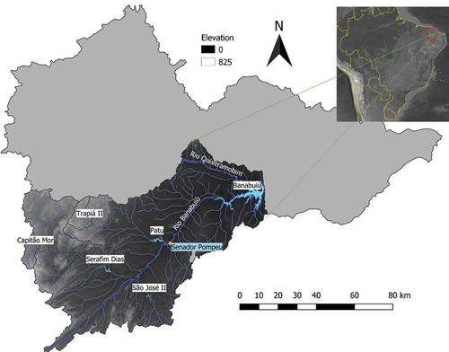
This study is focused on the part of the Banabuiú catchment upstream of the Senador Pompeu gauging station, which has an area of 4524 km². The five reservoirs located in this area are Capitão Mor, Patu, São José II, Serafim Dias and Trapiá II (Fig. 1). The Banabuiú reservoir is also included, which is the first reservoir downstream of Senador Pompeu and the largest reservoir in the Banabuiú catchment. The capacity, incremental drainage area and total drainage area of each reservoir are given in Table 1. These reservoirs present a low hydrological connectivity most of the time, which is why the precipitation on incremental drainage areas is more important for water supply to the reservoir than the precipitation on the total upstream area. Only when the reservoir volume reaches the capacity of the reservoir and spillway overflow occurs does hydrological connectivity occur (Lima Neto et al. 2011, De Toledo et al. 2014, De Toledo and Alcantara 2019). In that case, Capitão Mor is hydrologically connected to Serafim Dias, and Trapiá II becomes hydrologically connected to Patu. However, since our focus is on drought propagation, in the periods of interest the reservoirs are not filled to capacity and the system is hydrologically disconnected.

Table 1. Reservoir capacity and drainage area (see Fig. 1 for their locations). The incremental drainage areas are used for precipitation data and the total drainage area is used in the downstreamness analysis

Reservoir	Capacity (hm^3)	Incremental drainage area* (km^2)	Total drainage area (km^2)
Banabuiú	1601	4373	14 250
Capitão Mor	6	112	112
Patu	72	901	1031
São José 2	29	225	225
Serafim Dias	43	1507	1619
Trapiá II	18	130	130

*The incremental drainage area (or incremental basin) is the drainage area of the reservoir excluding the drainage area of other, more upstream reservoirs. The total drainage area of Patu consists of the incremental drainage areas of Patu and Trapiá II, for example. Unmonitored reservoirs are not taken into account for the incremental areas, because there is no data about their volumes and hydraulic connectivity.

2.2 Data collection

The study period is from January 2000 until August 2019, and was selected based on the availability of data on precipitation, streamflow and reservoir volume. Daily data for incremental precipitation and reservoir volumes (hm³) were obtained from the Foundation of Meteorology and Water Resources of Ceará (FUNCEME 2019). Incremental precipitation is the precipitation that takes place only in the sub-catchment of a reservoir or streamflow gauge, excluding sub-catchments of other upstream reservoirs (see Fig. 1 and Table 1). Streamflow data were obtained from the National Water Agency (ANA 2019). Streamflow data (m³/s) at Senador Pompeu gauging station were available from March 1973 until August 2019, which was used as the final month in this analysis. This streamflow gauging station is the only one in the studied reservoir network. Incremental precipitation data (mm/d) were available from January 1974 until November 2019. Reservoir data were used beginning in January 2000. Before January 2000, it was impossible to apply the method of filling reservoir data gaps, which is described in the Supplementary material (S1). The distribution of the reservoir data gaps is shown in Section 3.3. The quality of the data became better in general from 2000. Furthermore, most of the monitored reservoirs were already built in the Banabuiú catchment from 2000. The monitored reservoirs, which were constructed after 2000, are not part of the study area.

For the streamflow and precipitation data, the data gaps were filled with zero values, since these data gaps were mostly found in the dry season, when the precipitation data mainly consist of zeroes and the rivers dry completely out in the study area. This makes it likely that filling the data gaps with zeroes is valid. For streamflow, there were always measurements at least once every 1 or 2 months. For precipitation, there was only one data gap, of 18 d in July (incremental basin of Patu).

After interpolation, the data were transformed into monthly datasets. This resulted in the datasets shown in Table 2. For streamflow and precipitation, both the full time series and a subset starting from January 2000 were created. In the end, the subset was used for the analysis, but the longer datasets were used to investigate the implications of this decision for the objectives of this study, the results of which are shown in the Supplementary material (S2). To generate the results reported in Section 3, only the datasets covering January 2000–August 2019 were used.

Table 2. Monthly datasets used for analysis (FUNCEME, 2019, ANA, 2019)

Type	Dates	Variables	Names
Reservoirs	January 2000–August 2019	Volume at the end of the month (hm^3)	1. Banabuiú 2. Capitão Mor 3. Patu 4. São José II 5. Serafim Dias 6. Trapiá II
Streamflow	March 1973–August 2019 January 2000–August 2019	Average streamflow (m^3/s)	7. Senador Pompeu
Precipitation	January 1974–August 2019 January 2000–August 2019	Total precipitation (mm)	8. Incremental sub-catchments of: 9. Banabuiú 10. Capitão Mor 11. Patu 12. São José II 13. Serafim Dias 14. Trapiá II 15. Senador Pompeu

2.3 Standardized indices

In this study the SPI, SSI and SRSI were used to define when a drought occurred (start, duration and end) and how severe the drought was. Each index gives the anomalies of the variable of interest based on the historical data for that variable. For instance, the SPI, developed by McKee et al. (1993), of an area gives the anomaly in precipitation based on the historical precipitation data of that area. Seasonality is eliminated from the analysis by comparing a value for a given month with the other values in the dataset for the same month. How they were calculated is explained in more detail as follows.

The historical precipitation data forms a gamma distribution, which was transformed to a normal distribution with mean 0 and standard deviation 1. The value of the SPI was then calculated for each month. The drought categories corresponding to the different SPI values are shown in Table 3. A drought is defined as a period during which the SPI is continuously negative and reaches a value of −1 or less. The drought begins when the SPI drops below 0 and ends when the SPI becomes positive again after having reached a value of −1 (McKee et al. 1993). The magnitude of the drought is the sum of all monthly SPI values during the drought period.

Table 3. Drought Categories (McKee et al. 1993)

SPI/SSI/SRSI values	Drought category
0 to −0.99	Mild drought
−1.00 to −1.49	Moderate drought
−1.50 to −1.99	Severe drought
< −2.00	Extreme drought

SPI: Standardized Precipitation Index; SSI: Standardized Streamflow Index; SRSI: Standardized Reservoir Storage Index.

SPI can be calculated at various time scales (number of months). Smaller time scales could capture seasonality, while the larger time scales give the more long-term structure of the drought. The SPI for longer time scales is often more correlated with hydrological drought indicators (Keyantash 2018). To see responses in hydrology, often 12-month SPI is found to be the most appropriate to use, so this time scale was used here. The 12-month SPI value means that for the SPI of a given month, a combination of this month and the 11 preceding months is used in the calculation (WMO 2012).

In this study the SPI generator of the National Drought Mitigation Centre (NDMC 2018) was used to calculate both the SPI and the SSI at the 12-month time scale. This program fits the data to a gamma distribution and then transforms this into the standardized index. For both precipitation and streamflow, the gamma distribution fitted best to the data. This was tested using the fitdistrplus package in R (Delignette-Muller and Dutang 2015). The normality of the distribution of the resulting SPI and SSI were tested using the Shapiro-Wilkinson test.

For monitoring reservoir drought, Gusyev et al. (2015) proposed to use SRSI, which works in the same way as the SPI and SSI. Gusyev et al. (2015) combined reservoir volume data with reservoir inflows, adding the two variables to produce the input time series for SRSI. In this study, however, only reservoir volume is used as input for the SRSI calculation. The gamma distribution did not give a good fit for this dataset. Instead, the beta distribution was used to fit the data. To use this distribution, the data needed to be between 0 and 1, so the scaled volumes were calculated using the following equation:

(1) $\mathrm{S}\mathrm{c}\mathrm{a}\mathrm{l}\mathrm{e}\mathrm{d}\mathrm{X}=\frac{\mathrm{X}-\mathrm{m}\mathrm{i}\mathrm{n}\left(\mathrm{X}\right)+0.00001}{\mathrm{m}\mathrm{a}\mathrm{x}\left(\mathrm{X}\right)-\mathrm{m}\mathrm{i}\mathrm{n}\left(\mathrm{x}\right)+0.00002}$(1)

where X is the data, in this case reservoir volume. The values 0.00001 and 0.00002 were added because 0 and 1 were not acceptable values for the beta distribution and these values are small enough to not influence the data. Other than that, the same method used for the calculation of SPI and SSI was applied, and the 12-month time scale was also used. Since this is a new method, the implications of the choice of time scale for the objectives of this study were also investigated, by comparing the results to a 1-month and 24-month time scale; the results of this investigation are shown in the Supplementary material (S3). Furthermore, a check was done to confirm that the SRSI had a normal distribution, using the Shapiro-Wilkinson test.

2.4 Downstreamness

To understand how the water availability distribution over the reservoir network develops both during and following periods of drought, a spatial analysis was done to see where most water is stored, using the downstreamness concept (Van Oel et al. 2011). The downstreamness of a location is the ratio of its upstream catchment area to the entire river basin area. The downstreamness of a function on the basin, such as water availability, is defined as the downstreamness-weighted integral of that function divided by its regular integral (Van Oel et al. 2011). This analysis was done on a monthly time scale to include seasonal variation. The downstreamness of individual reservoirs was calculated using the following equation (Van Oel et al. 2011):

(2) $\mathrm{D}\mathrm{x}=\frac{{\mathrm{A}}_{\mathrm{u}\mathrm{p}\mathrm{s}\mathrm{t}\mathrm{r}\mathrm{e}\mathrm{a}\mathrm{m},\mathrm{x}}}{{\mathrm{A}}_{\mathrm{t}\mathrm{o}\mathrm{t}\mathrm{a}\mathrm{l}}}\times 100\mathrm{\%}$(2)

where D_x is the downstreamness of location x (%), A_upstream,x is the area upstream of location x (km²) and A_total is the total area of the catchment (km²). With the downstreamness of the locations, the downstreamness of the stored volume and storage capacity of the reservoirs was also calculated using the following equations (Van Oel et al. 2011):

(3) ${\mathrm{D}}_{\mathrm{S}\mathrm{C}}=\frac{{\sum }_{\mathrm{x}=1}^{\mathrm{n}}\mathrm{S}{\mathrm{C}}_{\mathrm{x}}{\mathrm{D}}_{\mathrm{x}}}{{\sum }_{\mathrm{x}=1}^{\mathrm{n}}\mathrm{S}{\mathrm{C}}_{\mathrm{x}}}$(3)

(4) ${\mathrm{D}}_{\mathrm{S}\mathrm{V}}=\frac{{\sum }_{\mathrm{x}=1}^{\mathrm{n}}\mathrm{S}{\mathrm{V}}_{\mathrm{x}}{\mathrm{D}}_{\mathrm{x}}}{{\sum }_{\mathrm{x}=1}^{\mathrm{n}}\mathrm{S}{\mathrm{V}}_{\mathrm{x}}}$(4)

D_SC and D_SV are the downstreamness of storage capacity and storage volume, respectively (%). SC_x and SV_x are the storage capacity and storage volume at location x (hm³) and n is the number of locations (reservoirs) in the catchment for which the downstreamness is determined. Comparing D_SC and D_SV shows whether more water is stored upstream or downstream (during droughts). If D_SV is smaller than D_SC, more water is stored upstream; when D_SV is larger than D_SC, more water is stored downstream (Fig. 2).

Figure 2. Schematic depiction of three situations of reservoir filling rates for a river basin with two reservoirs: (a) if the filling rates are equal, the downstreamness of the stored volume (D_SV) equals the downstreamness of storage capacity (D_SC); (b) if the filling rate of the upstream reservoir is greater than that of the downstream reservoir, D_SV is less than D_SC; and (c) if the filling rate of the upstream reservoir is less than that in the downstream reservoir, D_SV is greater than D_SC. Reprinted from Van Oel et al. (2018)

3 Results

3.1 Precipitation

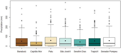
In Fig. 3, the yearly total precipitation and climatology are shown for the period from January 2000 until August 2019. In Fig. 3(b), the yearly cycle of wet and dry seasons can be distinguished. When looking at the yearly total precipitation (Fig. 3(a)), it was found that in the largest part of the catchment, the three wettest years in this period were 2004, 2009 and 2011, while the driest years were 2001, 2010 and 2012. However, it should be noted that the incremental basin of Capitão Mor received little precipitation in the years 2006–2009, which is remarkable, since 2009 is one of the wetter years in general. The box plots showing total monthly incremental precipitation for each catchment (Fig. 4) are quite similar for all reservoirs and the gauging station, except for Capitão Mor, where in general lower values were found.

Figure 3. (a) Total annual precipitation of the incremental basins of the reservoirs and the gauging station (Senador Pompeu), showing wetter and drier years and some variability between the areas; and (b) climatology of the incremental basins as average precipitation per month, showing the wet and dry seasons

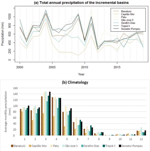
Figure 4. Box plot of the total monthly incremental precipitation; the black dots represent the mean. Capitão Mor stands out because of the lower values in general

SPI-12: 12-month Standardized Precipitation Index.

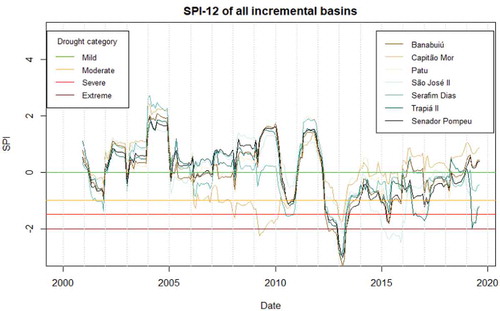
The monthly total precipitation was transformed into the SPI using the SPI generator (NDMC 2018). The normality of the results was tested using the Shapiro-Wilkinson test with alpha = 0.05, which had good results for SPI-12. Normality can be assumed for precipitations in all incremental basins except Serafim Dias. For Serafim Dias, the p value for the normality test was 0.0003 in February. However, the p values of the other months were all above (or very close to) 0.05. The resulting SPI-12 values are shown in Fig. 5. Most SPI values follow approximately the same pattern, but the SPI of the incremental basin of Capitão Mor stands out in the period from 2007 to 2010, where a drought occurs while the other SPI values are mostly higher than zero, indicating wetter conditions than normal. Multiple droughts can be observed from this figure, although some do not occur in all incremental basins. A clearer overview of the droughts will be given in Section 3.4, where they are compared to the hydrological droughts.

Figure 5. SPI-12 of the incremental basins of the reservoirs and Senador Pompeu gauging station; the horizontal lines represent the upper limits of the drought categories as given in Table 3

3.2 Streamflow

The monthly average streamflow is shown in Fig. 6, along with the precipitation in the incremental basin for the period from January 2000 until August 2019. In this period, there were no data gaps in the time series. The graph shows the seasonality in the area by alternating high and low flows or in some months no streamflow at all. The streamflow peaks follow quickly after the highest precipitation peaks. In some years, the streamflow peaks are lower or do not occur at all, indicating streamflow drought in these years. Interesting years that are likely to be considered streamflow droughts are 2000–2001, 2006, 2010 and 2012–2019 (the end of the dataset). Some basic statistics of the streamflow data is given in Table 4. This shows generally no or low flow, with some larger peaks as a response to rainfall.

Figure 6. Average monthly streamflow (m³/s) at the Senador Pompeu gauging station, with the total monthly precipitation (mm) in blue

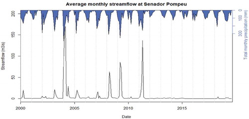
Table 4. Statistical summary of the monthly streamflow data

Mean	5.34
Standard deviation	20.70
Coefficient of variation	3.88
Median	0.63
Minimum	0
1^st quarter	0.31
3^rd quarter	1.63
Maximum	169.61
% of zero values	15.3

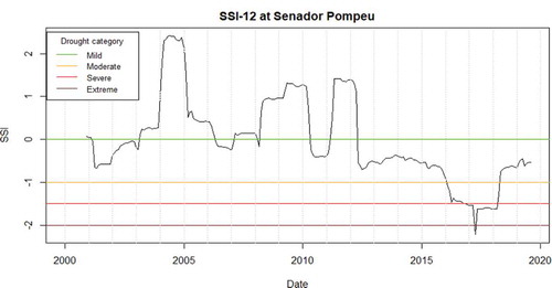
Figure 7 presents the SSI for Senador Pompeu gauging station, and it can be seen that indeed the periods mentioned before are relatively dry, with SSI values below zero. However, only one period can be classified as a drought. This drought starts in May 2012 and has not yet ended as of August 2019, which is the end of the analysed period. The lowest point was reached in January 2017, with an SSI value of −2.22, indicating extreme drought.

Figure 7. SSI-12 of the Senador Pompeu gauging station; the horizontal lines represent the upper limits of the drought categories as given in Table 3

SSI-12: 12-month Standardized Streamflow Index.

3.3 Reservoirs

The reservoir data starting from the year 2000 were used. The gaps in the data were filled using linear interpolation. The distribution of the gaps and the largest gap in the data of each reservoir are shown in Fig. 8. The data quality is quite good, although there are still some gaps in all datasets. Most of the gaps are found in the first 5 years of the time series; during this time, the data for São José II especially contained some large gaps. However, the interpolation method used is still assumed to give an acceptable result for filling these gaps.

Figure 8. Daily reservoir volumes (hm³) and the inserted values for the missing data, calculated through linear interpolation. In the title above each graph, the percentage of missing data points is given

After filling the data gaps, the volume (hm³) on the last day of each month was used for the monthly datasets. These data are shown as a percentage of the reservoir capacity in Fig. 9, to make it easier to compare the reservoirs with different capacities (Table 1). This value is sometimes higher than the capacity given in the data, which means that spillway overflow occurred at these moments. This does not matter for the SRSI analysis, since the capacity is not used. For calculating the downstreamness, these parts that are above capacity are assumed to not be of much influence, as the analysis is focused on extreme values during the droughts.

Figure 9. Percentage of the reservoirs that is filled on the last day of the month. The driest periods are of interest for this study, specifically the one starting in 2011–2012. Note the difference in time it takes for the reservoirs to be depleted and the steepness of the graphs from this point

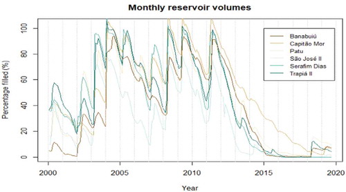
The lower values in Fig. 9 are the interesting point when looking at droughts. Some interesting, relatively dry years are 2000, 2002, 2003, 2007 (mostly for São José II) and 2013–2019. Banabuiú reservoir is less filled than the other reservoirs at the start of the analysis (2000–2002) and in 2004, but after that a similar pattern to the other reservoirs is seen. São José II seems to respond most quickly to drier circumstances in 2007 and 2013, while Capitão Mor has the slowest response in 2013. However, the graph for São José II is lower than the other ones during most of the period. To be more certain about this it is important to compare these data to the precipitation in their incremental catchments, which can be found in the next section. Recovery from drought situations seems more equal for all reservoirs. Nevertheless, in 2018, there appears to already be some recovery from the drought in Banabuiú, Patu and Trapiá II, while Capitão Mor and São José II do not show any increase in volume until 2019 and Serafim Dias is still completely empty at the end of the dataset (31 August 2019).

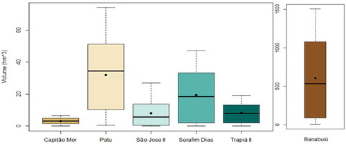
The box plots in Fig. 10 presenting reservoir volumes show that the range of data for all reservoirs is from (very close to) zero up to approximately their capacities (Table 1), so it shows the size of the reservoirs. Note that the box plot for Banabuiú is shown in a different graph, as it is much larger and including it in the same graph would make it impossible to see the shape of the other box plots. The mean and median are close to each other and around the middle of the range, but there is a slight skew to lower values for Banabuiú, São José II and Serafim Dias.

Figure 10. Box plots of reservoir volumes; the black dots represent the mean (2000–2019). The values range from approximately zero to the reservoir capacity

The SRSI was calculated by fitting the data to a beta distribution and transforming it to the standardized normal distribution for a 12-month time scale. Testing the normality of the resulting SRSI using the Shapiro-Wilkinson test gave good results (for all months, p value > 0.05) for Banabuiú, Capitão Mor, São José II and Trapiá II. The test was acceptable for Patu, with all p values at least > 0.025 and most > 0.05. For Serafim Dias, p values for 6 months (June to October and December) were below 0.05, but all remained above 0.025. This is less acceptable for assuming a normal distribution, so this was taken into account when analysing the results.

The SRSI is shown in Fig. 11. The only period that can be classified as a drought, reaching an SRSI of lower than −1, is the most recent dry period identified from Fig. 9. For all reservoirs the drought started in 2013 or 2014, shown by the first moment the SRSI dropped below zero. Table 5 gives more information about when the drought started and its magnitude. The reservoirs Trapiá II, Patu and Banabuiú reached the lowest level first (April, May and June 2017, respectively) and also started to recover first (April, May and April 2018, respectively). São José II and Capitão Mor follow the same pattern, but later (reaching the lowest point in August 2017 and August 2018 and starting to recover in August 2018 and August 2019, respectively). The pattern of Serafim Dias is slightly different. The drop to the lowest point (at the end of 2017) is less steep than for the other reservoirs, and at the end of the analysed period the volume is still zero (Fig. 9), so there is no recovery yet. Furthermore, for this reservoir the approach used did not result in a normal distribution, making it more difficult to draw conclusions from these results. It should be noted that even if a recovery for the other reservoirs is mentioned, none of them had reached an SRSI of 0 yet as of August 2019, meaning that the drought has not ended yet for any of the reservoirs. The other possible droughts mentioned in the description of Fig. 9 are not found by this SRSI approach. This is most remarkable for Banabuiú, since (as Fig. 9 shows) the reservoir empties almost entirely in 2001, with volumes declining from 50 hm³ (3.1%) in January to 10 hm³ (0.6%) in December. The severity of the later drought has most likely greatly influenced the distribution, making 2001 not dry enough to be qualified as a drought.

Figure 11. SRSI-12 of the reservoirs; the horizontal lines represent the upper limits of the drought categories as given in Table 3. More information about the drought onset and magnitude is given in Table 5

SRSI-12: 12-month Standardized Reservoir Storage Index.

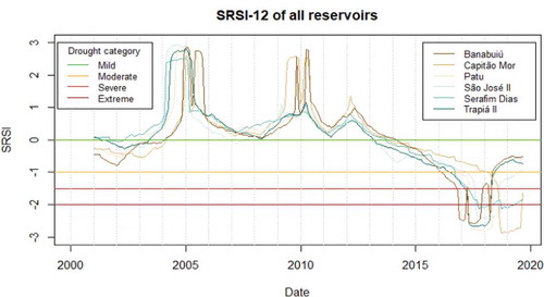
Table 5. SRSI drought onset, peak and magnitude. The drought peak gives the moment when the lowest SRSI value is reached. These values were always below −2, indicating an extreme drought

Reservoir	Drought onset	Drought peak	Drought magnitude
Banabuiú	February 2014	June 2017	69.13
Capitão Mor	October 2013	September 2018	65.65
Patu	February 2013	December 2017	72.58
São José II	February 2013	December 2017	79.02
Serafim Dias	September 2013	September 2017	82.20
Trapiá II	March 2013	July 2017	77.18

SRSI: Standardized Reservoir Storage Index.

3.4 Comparison of droughts

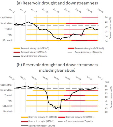
To compare the results the reservoirs are ordered in three clusters according to their hydrologic connections, as seen in Fig. 12. There are links between Capitão Mor and Serafim Dias and between Trapiá II and Patu. São José II is not hydrologically connected to other monitored reservoirs upstream of Senador Pompeu. It should also be noted that these connections do not really exist except for when the reservoirs are at their capacities. The rest of the time the water is used before it can reach the next reservoir. In this section, the meteorological drought (SPI) periods are compared to the hydrological drought (SSI and SRSI) periods. These periods are shown in Fig. 12 with different colours for different drought categories (Table 3), but moderate and severe droughts are taken together as a category where the value of the standardized index is between −1 and −2.

Figure 12. Drought periods for comparing meteorological to hydrological drought, ordered following the flow directions shown in the flowchart on the right (water flows downward). Note the time between the drought onsets and drought peaks (see also Tables 5 and 6)

SPI: Standardized Precipitation Index; SSI: Standardized Streamflow Index; SRSI: Standardized Reservoir Storage Index.

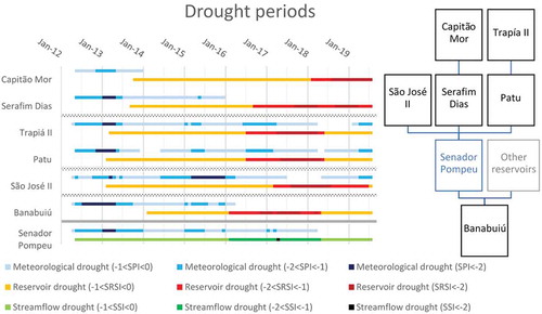
Not all meteorological droughts develop into hydrological droughts. Only one hydrological drought is found for all reservoirs and the gauging station (Fig. 12), while there are multiple meteorological droughts in their incremental basins. Only the meteorological drought starting in April/May 2012 developed into a hydrological drought. This meteorological drought became an extreme drought (SPI < −2) at the end of 2012 or in the first half of 2013 in all incremental basins except that of Capitão Mor. In the incremental basin of Capitão Mor, the drought did not reach an SPI of −2 and it only lasted until the end of 2013, while the drought continued or started again after short relatively wet periods in the other areas. In the incremental basin of Serafim Dias, which is in the same cluster as Capitão Mor, the meteorological drought ended at the end of 2015; it ended in early 2016 in the incremental basin of Banabuiú. For the other incremental catchments the meteorological drought lasted longer (ignoring the gaps in which there was a wetter period). For the incremental catchment of Senador Pompeu, the meteorological drought ended in March 2018, but the rest of the areas still experienced a meteorological drought at the end of the analysed period.

The streamflow drought (hydrological drought at Senador Pompeu gauging station) started in May 2012, showing the least delay after the start of the meteorological drought. For all the reservoirs, the hydrological drought started in 2013 or 2014 (Table 5). The response of the reservoir drought to the meteorological drought is very similar for the Trapiá II–Patu cluster and São José II, starting in March, February and February 2013, respectively. The cluster of Capitão Mor and Serafim Dias had a longer delay, with the reservoir droughts starting in October and September 2013, respectively. The longest delay is seen for Banabuiú, where the reservoir drought did not start until February 2014. All hydrological droughts started as mild droughts (standardized index between 0 and −1) for several years. After that, the droughts became more severe and all of them reached the extreme drought classification (standardized index < −2). By the time these hydrological droughts reached more severe classifications (standardized indices lower than −1), the most severe meteorological droughts had already ended. The meteorological droughts at that moment were still quite variable, ranging from normal (no drought) to severe (Trapiá II).

The time lag between the minimum SPI and minimum SRSI or SSI (moment of most severe drought) and the lag between the start of the droughts are presented in Table 6. For the start of the meteorological drought, April or May 2012 was used for all calculations. There were some earlier meteorological droughts, but this is the one that propagated into a hydrological drought. For Capitão Mor, this drought was also used for the minimum SPI, although there was a lower SPI value in an earlier drought. The values in this table show that the start of the hydrological drought happens within 2 years of the start of the meteorological drought, with the lowest being the streamflow drought after 1 month. The start of the reservoir drought at Banabuiú had a lag of 22 months after the start of the meteorological drought, which is the longest lag. The minimum values show longer lags, mostly over 4 years. At São Jose II only the lag is 2 years, but the precipitation peak in its basin occurred in 2015, while the minimum SPI was reached in 2012–2013 for in the other areas (see Figs 5 and 12). The streamflow drought has a similar lag to the reservoir droughts when looking at the minimum values for the standardized indices.

Table 6. Time lags between SPI and SRSI/SSI for the start of the drought and the minimum value

Reservoir/streamflow gauge	Lag meteorological-hydrological drought onset (months)	Lag minimum SPI-SRSI/SSI (months)
Banabuiú	22	51
Capitão Mor	17	67
Patu	9	59
São José II	10	24
Serafim Dias	16	55
Trapiá II	11	53
Senador Pompeu (streamflow)	1	49

SPI: Standardized Precipitation Index; SSI: Standardized Streamflow Index; SRSI: Standardized Reservoir Storage Index.

Lastly, it should be noted that for Capitão Mor there was a meteorological drought that reached the extreme category from 2006 to 2010, which did not propagate into a hydrological (reservoir) drought. However, when there was a less long and less severe meteorological drought later, this propagated into a hydrological drought in a similar way to those in the other areas. This hydrological drought continued until the end of the analysed period, long after the meteorological drought had ended.

3.5 Downstreamness

The downstreamness of the stored volume and storage capacity of the five reservoirs upstream of the Senador Pompeu gauging station have been calculated. The downstreamness of storage capacity (D_SC) is a constant value of 20.7%, since no new reservoirs were built from 2000 to August 2019 in this area and it is assumed that the capacity of the existing reservoirs stays the same. These capacities and the downstreamness of the locations of the reservoirs are given in Table 7. Next to that, the downstreamness was analysed for all six reservoirs, also including Banabuiú. It should be noted that there are more reservoirs upstream of Banabuiú that were not included in this analysis, since they are not part of the study area. The D_SC for this analysis was a constant value of 91.9%.

Table 7. Downstreamness of the reservoirs relative to the Senador Pompeu gauging station and relative to Banabuiú reservoir and their capacities

Reservoir	Downstreamness (%) Senador Pompeu = 100%	Downstreamness (%) Banabuiú = 100%	Capacity (hm^3)
Banabuiú	-	100	1601
Capitão Mor	2.48	0.79	6
Patu	22.79	7.24	65
São José II	4.97	1.58	21
Serafim Dias	35.79	11.36	41
Trapiá II	2.88	0.91	18

The downstreamness of stored volume (D_SV) is variable over the analysed period, which is shown in Fig. 13, represented by the black line. The grey horizontal line is the downstreamness of storage capacity. When D_SV < D_SC relatively more water is stored in the upstream reservoirs, while D_SV > D_SC means that relatively more water is stored downstream (Fig. 2). The most outstanding part of Fig. 13(a) is from 2013 until the end, when D_SV drops to 15% and then starts increasing again, but remains below the D_SC line, so more water is stored in the upstream reservoirs. This period corresponds to the hydrological drought periods shown in Figure. 12. The lowest point is reached in March 2016, which corresponds to the moment when the stored volume in the reservoirs starts to stabilize around zero. However, none of the reservoirs have reached their minimum volume yet at this point (Fig. 9).

Figure 13. Downstreamness of storage volume (black line) and capacity (grey horizontal line) relative to (a) the Senador Pompeu gauging station (Banabuiú reservoir not included) and (b) Banabuiú reservoir

In Fig. 14, downstreamness is plotted in the graph of the reservoir drought period. This also shows that the lowest SRSI values occurred later than the lowest D_SV. In fact, the D_SV starts rising again at the moment that the reservoirs reach more extreme drought classifications. In the beginning of 2019, the D_SV has increased until close to the D_SC, even though the reservoir drought, streamflow drought and meteorological drought (except for the Serafim Dias–Capitão Mor cluster) are continuing. In Figs 13(b) and 14(b)) Banabuiú reservoir is also included in the downstreamness analysis as the most downstream point. These graphs show the same general trend, but there is another drop in D_SV at the start until 2002 (only shown in Fig. 13(b)). This period was not classified as a drought using the standardized indices, but visual inspection of the data showed that this was also a relatively dry period (Fig. 9). It should also be noted that in Figs 13(b) and 14(b), Banabuiú is the only downstream reservoir, while the other reservoirs have very low downstreamness values (Table 6).

Figure 14. Comparing reservoir drought to downstreamness, a combination of Figs 12 and 13 (again (a) excluding and (b) including Banabuiú reservoir)

SRSI: Standardized Reservoir Storage Index.

When looking at the downstreamness of the reservoir clusters – thus comparing only two reservoirs to each other (Fig. 15) – it can be seen that the two clusters respond very differently to the drought. The Capitão Mor–Serafim Dias cluster (Fig. 15(a)) shows a drop in downstreamness, which had already started in 2011. At the end of the analysed period, Serafim Dias is empty, while Capitão Mor is not, resulting in a downstreamness of zero. The Trapiá II–Patu cluster (Fig. 15(b)), on the other hand, shows a high downstreamness during the drought period, meaning that relatively more water is stored downstream (Patu), while Trapiá II is empty for some time, since the downstreamness of 22.77% is the downstreamness of Patu (Table 7). However, in Fig. 15(b) a low downstreamness can be seen from 2000 until 2002, which was not identified as a drought but was still a relatively dry period.

Figure 15. Downstreamness of storage volume (black line) and capacity (grey horizontal line) relative to (a) the Senador Pompeu gauging station of the Capitão Mor-Serafim Dias cluster and (b)the Patu-Trapiá II cluster. The two clusters show very different responses to drought

4 Discussion

4.1 Drought periods

Our findings suggest that an extreme meteorological drought (reaching SPI < −2) is most likely to result in a hydrological drought, while other meteorological droughts do not necessarily cause a hydrological drought. The streamflow drought started a lot more quickly after the start of the meteorological drought than the reservoir droughts did (after 1 month compared to 9 months or more; Table 6). This shows that the reservoirs fulfil their purpose of supplying water at the start of this drought. However, after some years of (near) normal precipitation, the reservoir droughts continue and also the streamflow drought continues when the SPI-12 returns to normal. The hydrological droughts reach their most extreme values a long time after the most extreme SPI value (mostly between 4 and 5 years later; Table 6). This shows that the hydrological drought can disconnect from the meteorological drought, which was also observed by Oertel et al. (2018) in other semi-arid areas in Latin America. These values are also seen for the streamflow drought, which indicates that the reservoirs also influence its severity and duration, while the start is clearly influenced by the meteorological drought. This indicates that at some point, the natural hydrological (streamflow) drought becomes a human-modified hydrological drought (Van Loon et al. 2016). The analysed period is too short to conclude anything about the end of the drought, as the hydrological drought still continues. The meteorological drought on the other hand, has ended in at least part of the study area.

Therefore, it seems that it takes a long time for the reservoirs to fill up to normal levels after the end of a meteorological drought. This could be a benefit in some regions, if the precipitation provides enough water to users while also filling up the reservoirs. In semi-arid regions like Northeast Brazil even normal amounts of precipitation are low, while evapotranspiration and temperatures are high (Lemos and De Oliveira 2004). Thus, the reservoirs are essential for water supply in the dry season while, also, large amounts of water are required to fill the reservoirs again. Furthermore, the size of the reservoirs should be discussed. Banabuiú is by far the largest of the analysed reservoirs and it takes the longest to start drying up, but it is also the first one to reach severe and extreme drought classification (Fig. 12). This indicates that more water is retained upstream during the drought and this large reservoir cannot receive enough water. This is confirmed by the other analyses, discussed in the next sections. For recovery to normal levels it is, as mentioned before, difficult to draw conclusions already. So far, no clear differences can be seen between the reservoirs.

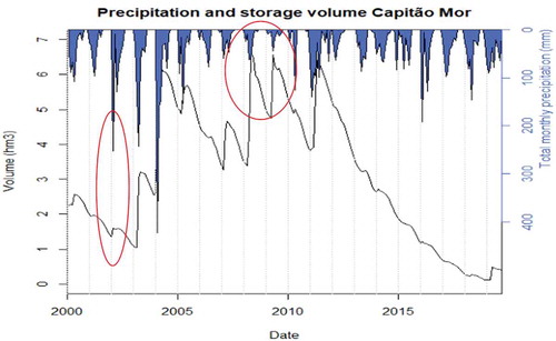
Lastly, there is one part of Fig. 12 that looks counterintuitive. This is the part on Capitão Mor, where there is a more severe meteorological drought from 2006 until 2011 (Fig. 5). This meteorological drought did not propagate into a hydrological drought, but the less severe meteorological drought after that (2012–2014) did (Fig. 12). This does not seem logical. A number of reasons can be considered to explain this. Firstly, the quality of the precipitation data could be considered, as the precipitation in the incremental basin of Capitão Mor is lower than in the rest of the study area. The significance of this difference was confirmed by the Kolmogorov-Smirnov test, with P values around 0. We learned that there is only one measurement station in that area, and spatial variability in the precipitation pattern could mean that these observations are not completely representative. Furthermore, it is more likely that the precipitation pattern would be similar to the rest of the area. From 2005 to 2010 especially, the precipitation is a lot lower (Figs 3(a) and 5)), while the reservoir still fills to capacity multiple times during this period, as seen in 2008 and 2009 (Fig. 16). In 2002, however, there was a large precipitation peak, to which the reservoir volume barely responded (Fig. 16).

Figure 16. Precipitation and reservoir volume of Capitão Mor, showing a misfit between the two datasets (red circles)

The area around Capitão Mor has somewhat different properties than the rest of the study area. It is at a higher elevation and has a different soil type, and the vegetation looked greener (Governo do Estado do Ceará 2007). The soil type around Capitão Mor is mostly Luvissolo (Lal 2017), a soil with a well-developed structure and high natural chemical fertility (Embrapa n.d.). The other soils found in the catchment are Agrissolo and Chernossolo. These differences are a second possible explanation for the interesting propagation of drought in this area. Possibly, more water is stored in the soil or other depressions in this hillier area, delaying the propagation of drought, but more information about the specific soil characteristics in these areas is needed before a conclusion can be drawn.

A third reason could be a change on the demand side instead of the supply side. Since there is still a drought downstream of Capitão Mor, it is likely that demand has increased. Higher water use could therefore also decrease the reservoir levels and be a reason for the reservoir drought. On the other hand, the gentler slope of emptying of this reservoir (Fig. 9) suggests a lower demand from this reservoir compared to the other reservoirs in the area. It would be interesting to investigate the demand side further, but this was outside the scope of the current study. No final conclusion can be drawn about this issue, but an error in the precipitation data is assumed to be the most likely reason for the anomaly.

4.2 Downstreamness

When the water is divided equally over the catchment relative to the reservoir capacities, the downstreamness of stored volume (D_SV) is equal to the downstreamness of storage capacity (D_SC). This is generally true in a normal situation. When a drought starts, the D_SV starts to decrease, so more water is stored upstream. This confirms that the downstream reservoirs dry up more quickly, while these are larger in general, which makes it logical that they take longer to empty. The most logical explanation for this is that water is retained upstream. The D_SV goes back up when either the reservoirs are filled again to an approximately equal percentage or the reservoirs are all almost empty. This occurred during the recent multi-year drought. The D_SV appears to return to values of a normal situation, but this is a new balance of an extremely dry situation instead (see Figs 9 and 14). Therefore, when looking at the whole area, downstream reservoirs are more affected at the start of a drought, but later during the drought, the effects are equally distributed between upstream and downstream. This confirms the hysteresis of the downstreamness of stored volume, identified by Van Oel et al. (2018). The D_SV decreases initially because of faster depletion of downstream reservoirs. To return to a balance (D_SV = D_SC), one might expect this to be caused by filling of these downstream reservoirs. However, in this analysis the balance is achieved when stable, low water levels are reached in all reservoirs.

When looking at a very local scale, just considering two reservoirs, different results were obtained (see Fig. 15). This shows that it is not always true that a downstream reservoir is affected more. When looking at Serafim Dias (downstream) and Capitão Mor (upstream), the D_SV decreases at the start of the drought and stays low. The reason for this is that Serafim Dias empties completely and stays empty until the end of the period, while Capitão Mor always contains some water. This could be due to differences in management or demand. When looking at Patu (downstream) and Trapiá II (upstream), the D_SV is low during the dry period from 2000 until 2002, but it is higher than the D_SC during the entire recent drought. There is no clear reason why more water is stored downstream, but Figs 9 and 12 show that these reservoirs have similar responses at the same moments during this recent drought. It seems that Patu and Trapiá II are a lot more similar to each other than Serafim Dias and Capitão Mor are. This similarity is not caused by their capacities or the size of their drainage areas, which are a lot larger for the downstream reservoir in both cases (Table 1). It could be partly caused by environmental differences, like soil type and amounts of precipitation, which are mostly different around Capitão Mor (if the precipitation data is reliable). However, the general results showed that a drop in D_SV occurs at the start of a drought (Fig. 13), which corresponds more to the relation between Serafim Dias and Capitão Mor (Fig. 15(a)). Therefore, differences in management and demand are a more likely cause of these large differences.

According to Lemos and De Oliveira (2004), the amount of water that is released from the reservoirs is determined in consultation with water users, through informal commissions. The water users in the highlands benefit more from higher water levels in the reservoir to supply irrigation water throughout the season, while lowland farmers prefer a greater release of water to expand their planted area. This could be an explanation for the relatively higher levels at Capitão Mor. However, this management structure was still evolving when that paper was written. It would be interesting to investigate how these institutions and commissions have changed since 2004, especially during this most recent drought. This also fits the reservoir effects as described by Di Baldassarre et al. (2018). They suggest that increased water availability from reservoirs can also increase water demand, which then has a negative effect on the water availability. This causes difficulties during a drought, when the reservoir can no longer provide enough water to meet the rising demand.

4.3 Perceptual model

A perceptual model was developed based on the findings of this study (see Fig. 17). This shows how the drought propagates through a reservoir network. Figure 17 shows how the drought starts with a meteorological drought, which then develops into two types of hydrological droughts, of which the streamflow drought starts earlier than the reservoir drought. The reservoir drought also affects the streamflow drought, transforming it into a human-modified hydrological drought, which reaches its peak around the same time as the peak reservoir drought. Reservoir drought is always considered a human-modified hydrological drought in this study, since only man-made reservoirs are considered. The time lags between the meteorological and reservoir drought (both the onset and the peak) are more variable, depending on the capacity, downstreamness and management of the reservoirs. Indeed, the time lags between the different types of drought (meteorological, reservoir and streamflow droughts) will depend on the reservoir management practice.

Figure 17. Perceptual model of drought propagation through a reservoir network, with the yellow circles indicating the time between the meteorological and hydrological drought and the time between the drought onset and peak. On the blue circles, the spatial distribution of stored water between upstream and downstream is shown. Downstreamness means downstreamness of volume in this figure. A scheme of the system of reservoirs and the streamflow gauging station (in blue) is also provided

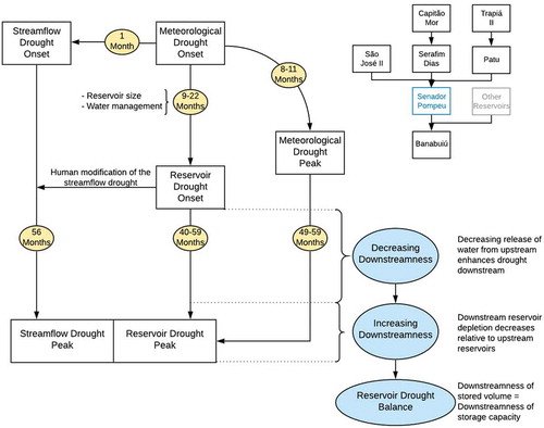
The spatial distribution of water stored in the reservoirs is shown in the blue circles of Fig. 17. Until the onset of the reservoir drought, water is distributed approximately equally between upstream and downstream reservoirs. After a decreasing downstreamness of stored volume, a new balance occurs following the reservoir drought peak. It should be noted that the values for the meteorological drought exclude the values of Capitão Mor (because of unreliable data) and São José II (because it has a later drought peak, which deviates from the general results).

There are plenty of examples of cascade reservoir modelling being applied to drylands (e.g. Güntner et al. 2004, Medeiros et al. 2010, Mamede et al. 2012). However, none of these studies evaluates the simulation of hydrological drought, which may hamper seasonal drought forecasting (Pilz et al. 2019) and drought assessment due to climate change. Therefore, this perceptual model, which is based on process knowledge about spatial and temporal drought development in a reservoir network, may be helpful for the improvement of cascade reservoir modelling in drylands. This is because governing processes, such as disconnected runoff generation under rather low catchment moisture conditions and drought-driven reservoir water use changes, may be incorporated and/or adjusted to simulate the found hydrological drought patterns.

5 Conclusions

The objective of this research was to investigate the effect of a network of surface-water reservoirs on the propagation of a meteorological drought into a human-modified hydrological drought in the Banabuiú catchment, Brazil. Therefore, temporal and spatial analyses of precipitation, streamflow and reservoir levels were conducted. For temporal analysis, standardized indices were used and compared directly, in which the developed reservoir drought index (SRSI) proved to be an effective method to analyse reservoir volumes as a standardized index. The spatial analysis was done using the downstreamness concept.

It can be concluded that storage of water causes a delay in drought propagation from meteorological to hydrological drought. Streamflow drought (SSI) responds faster to meteorological drought than reservoir drought (SRSI), but after this initial response, the streamflow drought develops in a similar way to the reservoir drought. The reservoir drought starts in a similar way for all reservoirs, but the drought develops in different ways depending on certain characteristics. Firstly, the downstreamness analysis shows that drought develops faster in more downstream reservoirs, while more water is retained upstream, until at some point the levels get so low that water is divided equally again. Secondly, even though it is not studied explicitly in this research, water use appears to influence the development of a reservoir drought, probably increasing the drought severity for higher water use. Thirdly, the capacity of a reservoir can have an influence, since the reservoir drought started later for the largest reservoir. However, this is also the most downstream reservoir, so the drought downstream started later but developed into a severe drought more quickly.

This study could be relevant for many other semi-arid regions with reservoir networks experiencing droughts, providing a new standardized reservoir drought index, process knowledge on spatial and temporal drought propagation, and a reference perceptual model of drought in reservoir networks. It is recommended for water managers in such semi-arid areas to include in their decision-making the implications for the downstream area of retaining water upstream. This could slow the development of drought in downstream regions, but it would speed up the drought propagation upstream, so this should be considered carefully.

Acknowledgements

We thank the Brazilian National Water Agency (ANA), the Foundation of Meteorology and Water Resources of Ceará (FUNCEME) and the Water Company of the State of Ceará (COGERH) for streamflow, rainfall and reservoir data, respectively.

Disclosure statement

No potential conflict of interest was reported by the authors.

Supplementary material

Supplemental data for this article can be accessed here

Additional information

Funding

The second author thanks the Brazilian National Council for Scientific and Technological Development (CNPq) for the post-doctoral scholarship [155814/2018-4]. The third and fourth authors received support from the Dutch Research Council (NWO) [project W 07.30318.016]; CNPq [155814/2018-4]; and the Netherlands Organisation for Scientific Research [W 07.30318.016].

References

- Agência Nacional de Águas (ANA), 2019. Séries Históricas de Estações. Available from: http://www.snirh.gov.br/hidroweb/serieshistoricas [Accessed 11 December 2019].
- Blöschl, G., et al., 2019. Twenty-three unsolved problems in hydrology (UPH)–a community perspective. Hydrological Sciences Journal, 64 (10), 1141–1158. doi:https://doi.org/10.1080/02626667.2019.1620507
- Byakatonda, J., Parida, B.P., and Kenabatho, P.K., 2018. Relating the dynamics of climatological and hydrological droughts in semiarid Botswana. Physics and Chemistry of the Earth, Parts A/B/C, 105, 12–24. doi:https://doi.org/10.1016/j.pce.2018.02.004
- Crausbay, S.D., et al., 2017. Defining ecological drought for the twenty-first century. Bulletin of the American Meteorological Society, 98 (12), 2543–2550. doi:https://doi.org/10.1175/BAMS-D-16-0292.1
- De Toledo, C.E. and Alcantara, N.R., 2019. Sensitivity of hydrological connectivity in a semiarid basin with a high-density reservoir network. Revista Ambiente & Água, 14, 4.
- De Toledo, C.E., de Araújo, J.C., and de Almeida, C.L., 2014. The use of remote-sensing techniques to monitor dense reservoir networks in the Brazilian semiarid region. International Journal of Remote Sensing, 35 (10), 3683–3699. doi:https://doi.org/10.1080/01431161.2014.915593
- Delignette-Muller, M.L. and Dutang, C., 2015. fitdistrplus: an R package for fitting distributions. Journal of Statistical Software, 64 (4), 1–34. doi:https://doi.org/10.18637/jss.v064.i04
- Di Baldassarre, G., et al., 2018. Water shortages worsened by reservoir effects. Nature Sustainability, 1 (11), 617. doi:https://doi.org/10.1038/s41893-018-0159-0
- Embrapa, n.d. Solos Brasileiros. Available from: https://www.embrapa.br/tema-solos-brasileiros/solos-do-brasil#collapse_zwhm_1 [Accessed 13 January 2020].
- Fundação Cearense de Meteorologia e Recursos Hídricos (FUNCEME), 2019. Portal hidrológico do Ceará. Available from: http://www.hidro.ce.gov.br/ [Accessed 14 January 2020].
- Governo do Estado do Ceará, 2007. Ceará em mapas. Available from: http://www2.ipece.ce.gov.br/atlas/lista/index.htm [Accessed 14 January 2020].
- Governo do Estado do Ceará, 2019. Portal Hidrológico do Ceará. Available from: http://www.hidro.ce.gov.br [Accessed 14 January 2020].
- Güntner, A., et al., 2004. Simple water balance modelling of surface reservoir system in a large data-scarce semiarid region. Hydrological Sciences Journal, 49 (5), 901–918. doi:https://doi.org/10.1623/hysj.49.5.901.55139
- Gusyev, M., et al., 2015. Drought assessment in the Pampanga River basin, the Philippines–Part 1: characterizing a role of dams in historical droughts with standardized indices. In: Proceedings of the conference on modelling and simulation (Vol. 29). Broadbeach, Australia.
- Huang, S., et al., 2017. The propagation from meteorological to hydrological drought and its potential influence factors. Journal of Hydrology, 547, 184–195. doi:https://doi.org/10.1016/j.jhydrol.2017.01.041
- INESP, 2009. Caderno Regional da Sub-Bacia do Banabuiú. Available from: http://portal.cogerh.com.br/wp-content/uploads/2018/09/Bacia-do-Banabuiú [Accessed 15 January 2020].
- Keyantash, J., 2018. The climate data guide: standardized precipitation index (SPI) [online]. Available from: https://climatedataguide.ucar.edu/climate-data/standardized-precipitation-index-spi [Accessed 16 January 2020].
- Kundzewicz, Z.W. and Kaczmarek, Z., 2000. Coping with hydrological extremes. Water International, 25 (1), 66–75. doi:https://doi.org/10.1080/02508060008686798
- Lal, R., 2017. Encyclopedia of soil science. Boca Raton: CRC Press.
- Lemos, M.C. and De Oliveira, J.L.F., 2004. Can water reform survive politics? Institutional change and river basin management in Ceará, Northeast Brazil. World Development, 32 (12), 2121–2137. doi:https://doi.org/10.1016/j.worlddev.2004.08.002
- Lima Neto, I.E., Wiegand, M.C., and de Araújo, J.C., 2011. Sediment redistribution due to a dense reservoir network in a large semi-arid Brazilian basin. Hydrological Sciences Journal, 56 (2), 319–333. doi:https://doi.org/10.1080/02626667.2011.553616
- Mamede, G.L., et al., 2012. Overspill avalanching in a dense reservoir network. Proceedings of the National Academy of Sciences, 109 (19), 7191–7195. doi:https://doi.org/10.1073/pnas.1200398109
- Marengo, J.A., Torres, R.R., and Alves, L.M., 2017. Drought in Northeast Brazil—past, present, and future. Theoretical and Applied Climatology, 129 (3–4), 1189–1200. doi:https://doi.org/10.1007/s00704-016-1840-8
- McKee, T.B., Doesken, N.J., and Kleist, J., 1993. The relationship of drought frequency and duration to time scales. In: Proceedings of the 8th Conference on Applied Climatology. Vol. 17, No. 22. Boston, MA: American Meteorological Society, pp. 179–183.
- Medeiros, P.H.A., et al., 2010. Modelling spatio-temporal patterns of sediment yield and connectivity in a semi-arid catchment with the WASA-SED model. Hydrological Sciences Journal, 55 (4), 636–648. doi:https://doi.org/10.1080/02626661003780409
- Mishra, A.K. and Singh, V.P., 2010. A review of drought concepts. Journal of Hydrology, 391 (1–2), 202–216. doi:https://doi.org/10.1016/j.jhydrol.2010.07.012
- NDMC, 2018. Downloadable SPI program. Nebraska-Lincoln: National Drought Mitigation Center. Available from: http://drought.unl.edu/MonitoringTools/DownloadableSPIProgram.aspx.
- Oertel, M., et al., 2018. Drought propagation in semi-arid river basins in Latin America: lessons from Mexico to the Southern Cone. Water, 10 (11), 1564. doi:https://doi.org/10.3390/w10111564
- Peter, S.J., et al., 2014. Flood avalanches in a semiarid basin with a dense reservoir network. Journal of Hydrology, 512, 408–420. doi:https://doi.org/10.1016/j.jhydrol.2014.03.001
- Pilz, T., et al., 2019. Seasonal drought prediction for semiarid northeast Brazil: what is the added value of a process-based hydrological model? Hydrology and Earth System Sciences, 23 (4), 1951–1971. doi:https://doi.org/10.5194/hess-23-1951-2019
- Van Loon, A.F., et al., 2016. Drought in the anthropocene. Nature Geoscience, 9 (2), 89. doi:https://doi.org/10.1038/ngeo2646
- Van Oel, P.R., Krol, M.S., and Hoekstra, A.Y., 2011. Downstreamness: a concept to analyze basin closure. Journal of Water Resources Planning and Management, 137 (5), 404–411. doi:https://doi.org/10.1061/(ASCE)WR.1943-5452.0000127
- Van Oel, P.R., Martins, E.S.P.R., and Costa, A.C., 2018. The effect of reservoir networks on drought propagation. European Water, 60, 287–292.
- Verdon-Kidd, D.C., et al., 2017. A comparative study of historical droughts over Texas, USA and Murray-Darling Basin, Australia: factors influencing initialization and cessation. Global and Planetary Change, 149, 123–138. doi:https://doi.org/10.1016/j.gloplacha.2017.01.001
- Wilhite, D.A., 1992. Planning for drought: a guidebook for developing countries. Climate Unit. Nairobi, Kenya: UN Environment Program.
- Wilhite, D.A., Ed., 2000. Droughts: a global assessment. London: Routledge.
- Wilhite, D.A. and Glantz, M.H., 1985. Understanding: the drought phenomenon: the role of definitions. Water International, 10 (3), 111–120. doi:https://doi.org/10.1080/02508068508686328
- World Meteorological Organization (WMO), 2012. Standardized precipitation index user guide. Geneva: World Meteorological Organization.