Modeling the system dynamics of irrigators’ resilience to climate change in a glacier-influenced watershed

ABSTRACT

Glacier-dependent streams and irrigation systems in the Hood River Watershed (HRW) are particularly vulnerable to climate change, as glaciers retreat and snowpack declines. We developed a system dynamics model designed to test and improve resilience of the HRW’s socio-hydrological system under Coupled Modeling Intercomparison Project 5 (CMIP5) climate change scenarios and irrigation infrastructure improvement, water banking, and water conservation. We hypothesized irrigators’ potential strategies would increase adaptive capacity by ensuring sufficient water resources for irrigation and minimum streamflow for fish habitat. Our model suggested predicted temperature increases will cause a lengthening of the dry season, causing streamflow declines, but adaptive measures have the potential to increase the capacity of the socio-hydrological system to “bounce back” from strains on streamflow given collective cooperation and the acceptance of agriculture–ecology tradeoffs. Hence, we found that system dynamics models offer useful tools for simulating localized potential impacts of climate change and developing possible solutions to improve resilience.

KEYWORDS:

• socio-hydrology
• coupled human–water system
• climate change
• drought
• adaptive management
• system dynamics

Editor S. Archfield Guest Editor M. Sivapalan

1 Introduction

Located in the transition zone between the high, desert plateau of Eastern Oregon and the temperate rainforest of the Western Cascades, Hood River faces an uncertain future of climate impacts. Whereas the western side of the river is impacted by climatic trends that often cause higher precipitation, the eastern side is situated closer to the rain shadow and receives less water. While future implications of climate change have been studied in the area (Bureau of Reclamation 2015), the need for mitigation of losses calls for greater effort towards creating and testing alternatives that address socio-hydrological processes. This paper attempts to engage in and contribute to this effort.

To begin, we asked two primary research questions that take into consideration both localized and generalizable findings. These are: “How can a system dynamics model (SDM) be constructed to model both the potential impacts of climate change and linked efforts by irrigators to mitigate potential hazards?” and “What can modeling irrigators’ potential strategies tell us about resilience and the capacity to adapt to climate change more generally?” These questions touch on the crucial coupling of human–water systems and the use of socio-hydrological models as it pertains to scenario forecasting and system resilience. It is important to bring together the social and hydrological systems, because they create an equilibrium through their interaction, which produces a unique and holistic system in itself. Thus, attempts to understand human–water and human–climate resilience by academics, policymakers, water managers, and engineers cannot fully conceptualize human resilience to climate change and water issues without also furthering climate and water resilience as well.

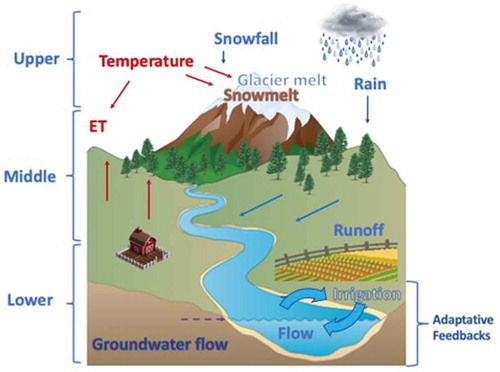
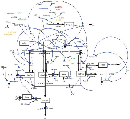
To further understand and articulate the processes and probable outcomes of hydroclimatic changes in the basin, as well as their concomitant effects on local agricultural producers, we created an SDM integrating crucial aspects of the socio-hydrological system as it pertains to irrigation. The model includes three levels: an upper climate system inclusive of snowmelt, a middle section including glacier ablation and precipitation runoff, and a lower basin level that involves irrigation withdrawals and streamflow. While there are different climatological scenarios based on simulated data using Coupled Modeling Intercomparison Project 5 (CMIP5) projections in the upper level, the lower level also incorporates feedbacks between irrigation systems and streamflow in which withdrawals become automatically dependent on flow. Our model presents a novel contribution to the literature on watershed SDMs by adding both snowpack and glacial melt, thus incorporating the whole cryosphere into the socio-hydrological context.

Gauging alternative, future scenarios helps deepen our understanding of the potential capacity for local residents to adapt to those circumstances, while gaining a sense of the adaptations that might best impact the coupled system itself. Thus, the current study goes beyond the basic social-ecological system as it addresses the adaptability and reorganization of the system that is expected to change rapidly with climate change (Robinson and Vahedifard 2016). We hypothesized that the river would be significantly impacted, and the irrigation systems with it, particularly on the eastern side. We also hypothesized that farming may have to be abandoned in some areas to maintain minimum flow levels unless adaptive strategies are considered. These efforts will help local water managers in a practical sense, while also providing a useful contribution to socio-hydrology by exhibiting a generalizable model with stylized relationships for coupled human–water systems using novel adaptation measures in a complex study site (in this case, a glacier-fed stream in a climatological transition zone).

2 Literature review

Socio-hydrology often involves the utilization of different kinds of models for understanding and projecting the evolving nature of the coupled human and water systems at a longer time scale rather than simulating a snapshot of the future (Srinivasan et al. 2017). These models, while imperfect, can offer holistic insight into the functions of system dynamics as humans leave their footprint on their environment and vice versa (Troy et al. 2015). Socio-hydrologists use statistical methods and SDMs, in particular, to understand the impacts of different scenarios and adaptive policy changes in human–water systems.

Tian et al. (2019, p. 16) used a statistical analysis to assess patterns of asymmetric water consumption during dry periods, discerning an “upward spiral” of human water consumption that a “new vision for water resources planning” could ameliorate. Studies using SDMs include the reuse of urban wastewater for irrigation in South Korea (Jeong and Adamowski 2016), the relationship between population rise and water resource demands in Ghana (Kotir et al. 2016), and glacial contributions to an agricultural basin in Iran (Ghashghaei et al. 2013). Other SDMs creatively engage with mutualist approaches to agricultural systems (Turner et al. 2016b), power generation (Feng et al. 2016), socio-economic development (Song et al. 2018), and saltwater intrusion (Lauriola et al. 2017).

No studies in socio-hydrology yet model glacial influence on irrigation systems in light of climate scenarios using SDMs, according to our research. While Kotir et al. (2016)’s insightful study illustrates the influence of climatological systems on variability in water availability for industry, it does not include a cryospheric component or a basin-scale analysis. On the other hand, while the important research by Ghashghaei et al. (2013) does include cryospheric modeling on the basin scale, it does not contain an integrated agricultural component. Similarly, Jeong and Adamowski (2016) combine a mechanistic physical model with human behavioral elements like land-use change, but their model describes an urban geography distinct from the questions of instream flows and canal losses that concern irrigation districts. Some studies do research cryospheric influence in irrigation systems (Nüsser et al. 2012, Carey et al. 2017), but not with SDMs. Thus, the present article, using an SDM to analyze the resilience of irrigation systems located in a glacially influenced watershed threatened by the impacts of climate change, is a novel contribution to the literature.

By “resilience,” we refer to a property of the system that depends on “the dynamics of system stability, the operation of structures and functions across spatial and temporal scales, and the ability of drivers on one level to influence change at other levels” (Davidson et al. 2016). These core conceptual elements assemble a definition of resilience as the ability of a system to “bounce back” from exogenous shocks that becomes heuristic for constructing representations of socio-ecological systems and disaster response (such as drought). They are also representable in an SDM through the presence of variable nodes as operational and relational structures and functions impacted, sometimes indirectly, by causal chains. Furthermore, SDMs, such as the present model, can include additional functions that can test a system’s adaptability, or “the capacity of people in a social–ecological system to build resilience through collective action” (Folke 2006, p. 262). According to the descriptions of resilience and adaptability described by Davidson et al. (2016), our model can be considered an adaptive resilience effort that would open a new direction towards a larger transformation of socio-hydrological relations in the basin.

SDMs are among the most frequently used models in socio-hydrology, along with agent-based models, because they articulate feedbacks within coupled systems that exhibit “big problems” of human–water coevolution (Sivapalan 2015). More specifically, SDMs can provide heuristic pedagogical tools to show how human behavior can and will impact the development of water systems, and how variability functions within a temporally specified system (Schlüter et al. 2012, Sivapalan 2015). As well, SDMs can offer long-term path analyses that avoid the mistakes and “back-firing” feedback of short-term planning (Turner et al. 2016a).

Developed by Massachusetts Institute of Technology (MIT) scientist Jay W. Forrester in the 1950s and subsequently taken up by General Electric and professionals in industry, military strategy, agriculture, biology, and ecology, SDMs use diagrams based on interconnected differential equations to exhibit the internal functions of a complex system expressed both graphically and quantitatively (Gustafsson 2017). Described as stock-and-flow systems or causal feedback loops, SDMs can represent essential relationships as they change over time based on alterations or perturbations at different points. Hence, uncertainty can be incorporated within nonlinear systems to produce a general model that examines how human interactions with environmental change can determine future conditions (Barlas 2009).

At the same time, Sivapalan (2015, p. 4801) notes that such models come with important qualifications: “The conceptualization, quantification and measurement of all variables, especially social variables, suffer from scale issues, a result of discrepancies between the scales at which they may be measured and the scales at which they are modeled.” Modelers often have to make important tradeoffs between precision, generality, and realism in defining the spatio-temporal boundaries of a system and its intended effects (Troy et al. 2015). To negotiate uncertainty in physical models while articulating more nuance than a conceptual model, Srinivasan (2015) offers a “stylized model” as a “simplified representation of the real world that aims to replicate the essential dynamics observed in one or more study sites, but does not attempt to calibrate and validate every variable.”

As “promising explorative tools that can help explore socio-hydrological dynamics and contribute to theory development,” stylized models have been used to examine feedback systems in flood risk (Di Baldassarre et al. 2015, p. 4779, Ciullo et al. 2017), conceptualize the dynamics of ancient systems (Kuil et al. 2016), and model the potential effects of climate extremes such as droughts (Di Baldassarre et al. 2017). SDMs with stylized characteristics, like the present effort, can then work under the assumption that while some of the variables may not be immediately verifiable, the trends modeled do present a heuristic, exploratory opportunity. If stylized models do not validate important variables, however, they are not useful, and this study recognizes those limitations by ensuring the necessary steps are taken to validate all critical variables.

3 Methods

3.1 Site selection

Located in the Columbia River Gorge that cuts through the Cascade Range on the Oregon border with Washington, Hood River relies on discharge from glaciers and snowpack for late-summer flows that nourish once-flourishing salmon runs and provide valuable water to farmers during the crucial months of the growing season. About 1248 km², the Hood River basin incorporates five irrigation districts (Fig. 1), producing close to $100 million in commodity sales annually. However, observations record the glaciers receding, while median snowpack levels reflect earlier peaks and sharper declines (Jackson and Fountain 2007, Fortner et al. 2009, Nolin et al. 2010, Bureau of Reclamation 2015, Frans et al. 2016). For farmers, this means losing water during an important dry period and potentially having to switch orchards to vineyards or other less water-intensive products.

Figure 1. Irrigation districts distributed through the Hood River Valley

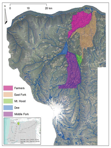
For local Native American tribes, the loss of streamflow could mean the complete collapse of already teetering salmonid runs, leading to cultural and economic impoverishment. Because of its unique place in the middle of the Cascade Range, the western part of Hood River feels the orographic effects of the mountains’ “rain shadow” more than the eastern part, which is generally drier. This unique geographical feature makes Hood River a vital habitat for four fish species considered threatened in terms of the Endangered Species Act (Bureau of Reclamation 2015, Salminen et al. 2016). These steelhead, bull trout, cutthroat trout, and spring Chinook require higher flows to ensure cooler water temperatures in order to swim up the Hood River and find spawning grounds. Since native people rely on the salmon for their livelihood and maintain water rights for in-stream flows to continue their traditional practices, water quantity becomes not just a moral issue but a potential legal quagmire (Galbreath et al. 2014). For local businesses that rely on recreation in the form of both farm tours and hiking around the glaciers, as well as some white-water kayaking, climate change will also present major problems.

Other studies have been conducted to examine the retreat of glacial mass balance on the mountain (Jackson and Fountain 2007, Fortner et al. 2009), as well as glacial contribution, and potential loss thereof, to the Hood River (Nolin et al. 2010). Indeed, such studies have contributed to a larger field of research on glacial vulnerability in the Pacific Northwest and the broader US (McCabe and Fountain 2013, Frans et al. 2018). However, studies regarding the potential impacts of retreating glaciers on the human systems that rely on them in the Mount Hood area have not been published outside of local reports. Hood River, then, becomes a valuable case study for the resilience of a socio-ecological system as the capacity for irrigators to “bounce back” from climate scenarios and drought while also integrating a balancing loop that ensures the sustainability of critical species habitat.

3.2 Data acquisition

Hood River is one of the most instrumented streams in the US. As a result of the Hood River Watershed Group’s efforts, as well, several studies of water quantity and availability have been conducted in the area (Christensen and Salminen 2013, Bureau of Reclamation 2015, Salminen et al. 2016). These studies and data installations proved instrumental in specifying an SDM to assess irrigation systems’ capacity to adapt to climate change in Hood River (Table 1). Developing stylized relationships enables an overview of a larger system involving multifarious nodes with built-in algorithms to allow for uncertainty and sensitivity analysis.

Table 1. Data used in the system dynamics model (SDM) of the Hood River Valley in Oregon, USA

Variable	Data source	Dates used
Streamflow	USGS Tucker Bridge (14120000), Middle Fork above West Fork, East Fork above Main Stem, West Fork near Dee (USGS 14120000)	1980–2004 (calibration), 2005–2020 (verification)
Precipitation (Rain/snowfall)	CMIP5/MACA simulated historical data, Climate Mapper Tool; gridMET (45.3965N, −121.6894E) observed historical data (MACA) (Gardiner et al. 2019)	1979–2005
Glacial discharge/DDF	Nolin et al. (2010)	2010
Snowpack	Mt. Hood SNOTEL Site #651 (SNOTEL)	2020
Irrigation withdrawals	Christensen and Salminen (2013)	2013
Temperature	CMIP5/MACA simulated historical data, gridMET observed (MACA)	1979–2005
Infiltration	Tang (1996), Suecker et al. (2000), Stähli et al. (2004)	1996–2004
Irrigation losses	Interviews with water managers, Christensen and Salminen (2013)	2013, 2020
Climate change scenarios	CMIP5/MACA (MACA)	2020

Observed precipitation, temperature, potential evapotranspiration, and mean monthly temperature data were generated from daily data gathered from the GridMET point (45.2965°N, −121.6894°E), located in the seasonally recurring snowpack near the Coe and Eliot glaciers that feed into the Middle Fork Hood River. GridMET provides a basin-wide, elevation-corrected climate grid for the study area at a 4 km² scale. These observed historical temperatures and precipitation from 1950–2005 were used to calibrate the model, along with average monthly snowfall estimates provided by the weather station at the Mount Hood SNOTEL Site (SNOTEL). Simulated historical conditions were generated using CMIP5 models to create a Base scenario. We relied on CMIP5’s 2050 and 2080 scenarios under the Representative Concentration Pathway (RCP) 4.5 conditions and RCP 8.5 conditions (representing reduced carbon emissions in the former case, and continued emissions in the latter) for calibration and scenario analysis, while reducing snowfall by an estimated 20% during the RCP 8.5 condition in accordance with the simulated drop in precipitation. CMIP projections were obtained using simulated daily data from MACA v. 2 METdata and bcc-csm1-1, which uses the r1i1p1 ensemble, available through the NW Climate Toolbox (Chegwidden et al. 2018).

Streamflow data were coupled with data on irrigation withdrawals at different points to measure the impacts of agriculture on streamflow (Christensen and Salminen 2013). We used a three-tiered conceptual model (Fig. 2) to show feedbacks between irrigation districts and streamflow in our model. While the schematic shows in detail the specificity of the irrigation system, to avoid overcomplicating our model, we simplified our model’s representation of the system by only showing the diversions that comprise the majority of the district (e.g. although the Middle Fork Irrigation District maintains water rights for some streams that flow from the East Fork, they only amount to 5.18 cubic meters per second [cms], so they were not factored in).

Figure 2. Three-tiered conceptual model of the system dynamics of the Hood River watershed

Because the model utilized a monthly time step in order to understand subtle changes on a decadal scale, the results can be generalized. Not all parameters are validated – for instance, groundwater was not validated because groundwater data are sparse and groundwater modeling is not the main goal of this model. At the same time, the most important and pertinent variables are specified in the present model. Capable of telling the story of what happens in the basin given different climate scenarios, this model is also used to explain why changes might occur, what strategies might be implemented to meet the demands of those new challenges, and what the results of those changes might be.

3.3 Model construction and parameterization

The SDM of the Hood River was divided into three sections (and one subsection) to fully explicate how the parts intersect (Fig. 2) (Fig. A1). The upper level comprises the climate, including the primary model drivers – precipitation and temperature – and their impacts on the snowpack and snowmelt. The middle level involves the effects of rain, snowmelt, and groundwater flows on streamflow at the top of the basin. A glacial ablation model was also included in the middle level. Lastly, the model uses real irrigation withdrawal data in order to ascertain, finally, the downstream flows of the mainstem Hood River through the city and into the Columbia River. By experimenting with different irrigation water withdrawals under different “water bank” scenarios, as well as irrigation infrastructure upgrades, we can see the feedback within a human–water system and model the outcomes of agricultural changes on streamflow.

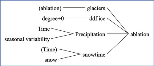
The first section of the model includes average monthly snow and rainfall (“seasonal variability” and “snow” parameters), as well as empirical monthly average temperatures, as lookup tables. Lookup tables bring an internal validity to the model logic, insofar as they represent actual diurnal variability without inference or interpolation. A simple parabolic wave lacks the exactitude of the actual monthly measurements provided by lookup tables. A degree day factor (DDF) equation following Nolin et al. (2010) (4.4 mm per degree Celsius over zero per day) was then used to track the extent of melt from the snowpack (Fig. 3).

Figure 3. Causes tree for glacial ablation showing feedback. DDF Ice indicates the degree day factor at which ice melts per degree above zero Celsius per day

The second part of the model, which includes upland flows, adds the hydro part to the hydroclimate SDM. As the melt flows from the snowpack, it is multiplied by the area of the sub-basin and the percentage of snowpack in the sub-basin by area. Thus, the linear measurement of snowmelt (i.e. the length of estimated water content of snow in millimetres over an area) is translated into a cubic measurement of water volume. A similar function is applied to the rain that flows into the watershed, with some losses to percolation in the groundwater estimated in correspondence with other studies about runoff and infiltration in similar coniferous forests and alpine and sub-alpine watersheds in Guangzhou, China (Tang 1996), the Colorado Rockies (Suecker et al. 2000), and Southern Switzerland (Stähli et al. 2004).

The glacial modeling relies on a similar DDF equation to the snowpack equation (11 mm per degree over 0 per day), multiplied by the glaciated area of the relevant sub-basins as described by Nolin et al. (2010). A feedback loop exists as well between the glaciers and the ablation rate, derived from an earlier study that found glacier discharge drops in relation to glacier retreat. Hence, as the glaciers decline, so does their contribution to runoff (Nolin et al. 2010).

A groundwater stock is also added as a conceptualization of the volume of water stored under the surface. The groundwater comprises infiltration from percolation of snowmelt, as well as rain across the span of the sub-basins. Water then moves from the groundwater stock into the streams via throughflow, becoming the baseflow for each tributary, as well as the mainstem itself. The amount of throughflow was determined by examining observed streamflow data contributed by local consultants. Since the flow meters at Tucker Bridge, West Fork near Dee, and East Fork above the Mainstem provide the best locations for identifying flow levels on the sub-watershed scale, they were used to estimate the throughflow. The average annual nadir of streamflow during the dry season, at which point no rain or snow could have influenced the streamflow, was located and used to approximate throughflow (Bureau of Reclamation 2015). As well, an evapotranspiration (ET) variable is developed using both observed and simulated scenarios from MACA to modify rainfall. Each ET scenario has built-in monthly values inputted to a lookup table that can be plugged into a modular 12-month variable, which then is subtracted from the variable for total rainfall over the basin (also a modular variable using observed or simulated data), thus rendering a generalized ET effect on total runoff.

The final segment of the model lies in irrigation, where the irrigators’ withdrawals impact the streamflow. Here, the tributary streams function as stocks in the same way as one might take a snapshot of a stream at a given time. There is water entering from runoff of snowmelt and rain, as well as throughflow. The stock empties immediately, and the flow itself is imagined as a fairly stable result of the general process of motion. Monthly measurements for irrigation withdrawals function on the outflow portion of the process in the same way as earlier lookup tables. Because farmers do not pull water out of the stream during the rainy season, actual monthly irrigation averages are used, providing different values for different months instead of averaging annual totals across 12 months. By using a lookup table with specific mean monthly water usage averages, the model provides a closer reflection of the naturally occurring socio-hydrological system, as opposed to a seasonal or annual scale, and shows the correlation between streamflow and shifts in precipitation and temperature (see Appendix B for full list of equations).

Such influences are important when experimenting with feedbacks in watershed–irrigation systems after the watershed model is complete, and while calibrating it. First, the irrigation districts are allowed to take as much water as their water rights demand, even if it leaves the stream with a negative flow. This helps us understand where, when, and how shortfalls in the water budget can be found, as well as the approximate quantity required to return to necessary values. Second, a tool is included to incorporate infrastructure improvements, vis-à-vis loss prevention. Next, a balancing loop is included comprising the calculation of the stream’s shortfall, and the subsequent substitution of that water from the irrigation flows. Thus, in the initial model, farmers may withdraw beyond the needs of instream rights. However, in subsequent scenario modeling, shortfalls (in the East Fork) are accommodated with sustainability measures like the balancing loop.

3.4 Calibration, specification and tuning

As mentioned above, the model’s logic is largely driven by a bidirectional movement. Firstly, climatological forcing of mean temperature and precipitation drove streamflow scenarios on a monthly scale in the first, top-down movement. Secondly, irrigation parameters were determined reflexively according to farmers’ needs and instream requirements in the bottom-up movement. The equations for DDF modeling were largely derived from an earlier study of the glaciers (Nolin et al. 2010), which is validated by another article on glacier contributions using a different isotope-based method (Frans et al. 2016). Based on studies of snowmelt and infiltration in other alpine and sub-alpine basins tested using sensitivity analysis, it was estimated about 15–25% of melt would enter streams directly, with the rest entering groundwater through infiltration or sublimating back into the atmosphere (Suecker et al. 2000, Stähli et al. 2004).

While the model uses metric units, it includes conversion variables to easily show conventional American measurement of cubic feet per second. In order to prevent variables from falling into negative numbers, we created algorithmic “if then else” functions that ensure zero as the lowest numerical possibility for variables other than temperature. For all lookup tables, a shadow variable of Time was modulated by 12 steps (i.e. 12 months in a year) using the Modulo function.

Internal model parameterization, specification, and logic were calibrated using climate and streamflow data from the period 1979–2005. This calibration period translates to climate scenarios in 2050 and 2080 based on the assumption of consistent crop types and general features of the basin. The model was initialized in steady state using observed data to determine its functioning, and then temperature, precipitation, and snow levels were altered in accordance with the simulated historical data and climate scenarios from CMIP5. Through this iterative process, and using the Nash-Sutcliff efficiency (NSE) to ascertain model accuracy, we calibrated the model to best reflect a precise record of the basic system, as well as results that could be validated through assessment of other studies.

3.5 Verification and validation

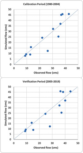
Verification in steady state took place by returning to observed flow levels from flow meters, snowpack levels from SNOTEL stations, and glacial runoff from Nolin et al. (2010) to ascertain the proximity of model outcomes and ensure that the model logic produced outcomes falling within a viable range of probability. After this iterative process involving the sensitivity analysis discussed in the next sections, the correlation between modeled mainstem streamflow using observed climate data and observed averaged monthly streamflow for a calibration period of water years from 1980–2004 produced an NSE of 0.73. Comparing the simulated flow to the observed flow for the verification period of water years from 2005 to 2019 produced an NSE of 0.675 (Fig. 4; Appendix A, Tables A1 and Tables A2, for coefficient tables). The model is particularly strong during the summer flows, which are especially important for predicting the hydrological dynamics of irrigation season. We also used other modeled predictions in basin studies conducted by federal agencies, local consultants, and the Watershed Group to assess our results by comparing them to results produced through alternative methods.

Figure 4. Observed streamflow and modeled streamflow (in cubic meters per second, cms) during the calibration period (1980–2004) and the verification period (2005–2019)

3.6 Sensitivity analysis

Lastly, sensitivity analysis was used on the rate of melt per day per degree over zero – DDF variables – to test their validity in relation to other variables, as well as the sensitivity of the whole system to them. Because these figures were derived from normalized equations across different glacierized mountain basins, they represent an estimate rather than an exact quantification. Hence, observations were made of the response of each function to reasonable variations in DDF, for both snow and ice, to document a plausible range of effects given each scenario. We then compared our model results using DDF combinations of ice and snow melt rates to the observed average monthly base flow at Tucker Bridge.

As shown in Table 2, the averaged values of 4.4 and 7.1 for snow and ice DDF used by Nolin et al. (2010) produced slightly different R² values, revealing that a sensitivity analysis could be used to fine-tune the model (Table 3). The snow DDF of 2.5 on the lower range of the scale provided a higher R² value when coupled with a 7.1 for ice, suggesting that a 9.1 ice DDF would overestimate glacial contributions. The same was true with the 4.4 snow DDF, bringing an adjusted R² value of 0.83. At the same time, an ice DDF of 11 offers only a slight reduction in streamflow, but produces better accuracy in modeling glacial discharge. Using a DDF of 2.5 (snow) and 11 (ice), then, enabled our model to predict upwards of 84% of simulated historic streamflow and explains within 86.5% of glacial discharge per Nolin et al. (2010), suggesting that it would provide a reasonable comparison. The same sensitivity analysis was used for infiltration rates and streamflow, due to the effects of generalization across different soil types. Since the Base simulation revealed that increased infiltration does not improve the model’s fitness, we maintained the ratio of snowmelt flowing directly into streams at 0.25 and rainfall at 0.175 (Appendix A, Table A2).

Table 2. Sensitivity analysis of degree day factor (DDF) snow and DDF ice (snow & ice), reporting R² values correlating to simulated streamflow and observed monthly flow at Tucker Bridge (1985–2005)

	DDF 4.4 & 7.1	DDF 2.5 & 7.1	DDF 4.4 & 9.1	DDF 2.5 & 9.1	DDF 4.4 & 11	DDF 2.5 & 11
R	0.91	0.91	0.91	0.92	0.91	0.92
R^2	0.83	0.84	0.83	0.84	0.83	0.84
Adj. R^2	0.82	0.83	0.82	0.83	0.82	0.83

Table 3. Comparison of glacial runoff degree day factor (DDF) to determine model fitness

	August–September discharge in m/month	Percent difference
Nolin et al. (2010)	4 290 000	–
Base (DDF 7.1)	3 036 460	−29.22
Base (DDF 9.1)	3 827 310	−10.79
Base (DDF 11)	4 558 000	+6.25

3.7 Scenario testing

As resilience is understood as the capacity to “bounce back” from a shock or perturbation within a system, we tested resilience to climate trends by observing whether farmers could maximize the amount of water used for agricultural production in a drought year while also maintaining minimum flow requirements for Steelhead and Cutthroat salmon rearing (Normandeau 2014). Thus, despite shocks to the natural system, farmers could ensure an appropriate socio-hydrological balance to avoid habitat die-offs and restore system functioning following the perturbation. To test the boundaries of the system, we introduced two scenarios by 2050. The Less Warm (LW2050) scenario represents simulations based on an RCP of 4.5, wherein radiative forcing caused by climate change stabilizes at 4.5 W/m², while the Hot/Dry (HD2050) scenario shows an RCP of 8.5, in which very few efforts to constrain greenhouse emissions have been successfully undertaken on a global scale (NOAA n.d.). The water managers must make a decision to risk a lawsuit and maintain their irrigation withdrawals on the East Fork or to sacrifice some of their yield for the good of the salmon by returning water to the stream.

The irrigators decide to undertake an iterative process, agreeing upon a bare minimum streamflow of about 2.24 cms in these trying times. Every time the water level drops below 2.24 cms, farmers decide to make necessary changes to draw the level back up. We also modeled other downstream feedbacks, returning irrigation losses instream through hypothetical infrastructure improvements, and through a Water Bank system derived from participant observation of Water Group meetings. The Water Bank scenarios are created by removing a given percentage of irrigation withdrawals from the East Fork Irrigation District, thus returning the flows to the stream, while infrastructure improvements are created as a variable turning irrigation losses back into streamflow.

3.8 Adaptive strategies for resilience

In assessing the water issues confronting the East Fork Hood River, we used three adaptive strategies identified during interviews with the Hood River Watershed Group and its participants: irrigation infrastructure improvements, water banking, and water conservation. Each of these measures offers insight into adaptability, representing the capacity “to build resilience through collective action” (Folke 2006, p. 262).

The first option is irrigation infrastructure improvements – especially improving piping canals that lose water to both evaporation and overflow – which would manifest the simplest adaptation that would require long-term investment. To examine and test the potential strategies for conservation, we homed in on the East Fork Irrigation District in particular, and built in a toggle for irrigation losses. Based on previous reports in the region, we determined that East Fork irrigation district losses, resulting from evaporation on open canals, amounted to upwards of 6.4 cms historically (Salminen et al. 2016). To model new infrastructure that would feed irrigation savings back into the stream given water-conserving pipelines, we included an irrigation savings variable that channels the losses back instream. Since infrastructure improvements would not compensate for total water loss given warming scenarios, they helped contribute to the study’s findings but are only included as an added benefit on top of other strategies, rather than as sufficient, stand-alone strategies in themselves.

Another option confronting the Hood River Watershed Group involves “water banking,” a system in which an alternating set of farmers allow their fields to go fallow, or grow less water-intensive crops, such as hay, during the season, in exchange for compensation from a general fund. As Parramond (2016) illustrates, water banking can develop out of collaborative social relations. Doing this would enable water to go back into the stream, theoretically resolving some important habitat conservation issues. To model these scenarios, we reduced the East Fork withdrawals by 10% (WB1), 20% (WB2), and 30% (WB3) in three different simulations using the Hot/Dry scenario.

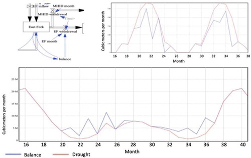
The final option is implementing a balancing feedback mechanism, which adapts to lower river flows by automatically lowering irrigation consumption in real time through water conservation. This option would involve more reflexive adaptation to streamflow minimums. Each of these would play a distinct role in the social relations of the basin. Using the method outlined above and inducing a drought by interrupting precipitation for the wet season, we simulated a perturbation to see how the system could respond reflexively. The balancing dual-feedback loop is inserted to return irrigation withdrawals instream in response to shortfalls of 2.53 cms that the farmers sacrifice to keep the minimum flows going, while most of their water rights continue to go towards crops.

3.9 Estimating impacts on agricultural production and economic losses without adaptation

While it is difficult to estimate the losses of agricultural production solely based on the decrease of instream flows, we developed a range of impacts based on the percentage of the market values sold between the years 2010 and 2017 ($77 117 000–$126 092 000) as the proportion of total irrigated acreage in Hood River taken up by the East Fork (57.86%) (USDA 2012, 2017). We used a linear relationship between water inputs and production to assess the financial losses with a reduction of in-stream flows. This rough estimation does not take into account any farmers’ adaptation strategies or other sources of water for augmenting irrigation flow.

4 Results

4.1 Change in snowpack and glaciers

The findings suggest two major issues. Firstly, snowpack will decline and peak earlier, shutting off late-summer streamflows. Secondly, glaciers will continue to recede at a faster pace, with ablation increasing at first but declining as glacier volume retreats. These two phenomena will represent a challenge to sustainability for irrigators who live downstream and rely on late-summer snowpack and glacial discharge. However, testing resilience within the system through a perturbation of drought conditions (zero rain across the rainy season) did indicate adaptive capacity through the incorporation of a compensatory mechanism triggered by low streamflow. Through this mechanism, farmers trade only enough irrigation withdrawals to ensure basic habitat protection, ensuring that agricultural production does not decline precipitously and that habitat remains safe as well.

A decrease in precipitation and increase in temperatures cut snow accumulation considerably on the mountain. Modeled snowpack based on observed historical climate data found 1.22 m, or about 48 inches, of SWE accumulation peaking in the month of May. While this number lies in the lower half of Mt. Hood snow years since 1980, it is just 8% over the median for the decade of the 2010s – 1.13 m (44.5 inches). Simulations of RCP 4.5 and 8.5 showed substantially diminished snowpack with very little deviation between them, accumulating to approximately 0.27 m (10.6 inches) in December, and then declining to virtually nothing by June (Fig. 5).

Figure 5. Causes strip for snowmelt in terms of snow water equivalent (SWE)

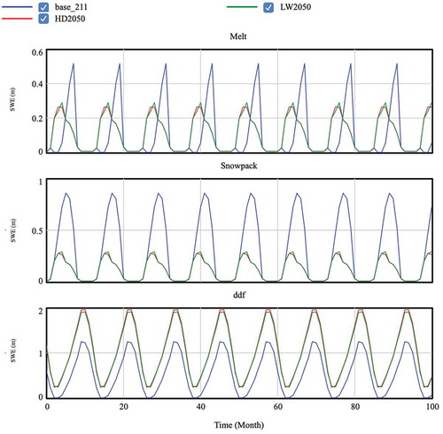
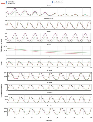
While warmer temperatures may bring increased melt to the glaciers, the reciprocal decline in glacier discharge resulting from a reduction in the glacier will counteract the higher discharge’s modest influence on streamflow under 2050 conditions for both RCP scenarios. Secondly, climatological forcing of temperature and precipitation causes streamflow to peak up to 3 months earlier (in January instead of March or April) and decline faster. These combined issues will lead to a decline in available irrigation water in summer.

Although glaciers are steadily declining, shortfalls are projected to occur most sharply for the non-glacier-influenced East Fork Irrigation District, with flows in the dry season dipping down to zero given current irrigation withdrawals (see “EF Outflow,” Fig. 6). The two scenarios Less Warm (LW2050) and Hot/Dry (HD2050) show earlier peaks and lower volume in snowpack accumulation and melt. These findings are also consistent with those of the Hood River Water Conservation Strategy (Salminen et al. 2016). As with all other streams, the East Fork peaks higher than the Base scenario, but declines more rapidly in warming scenarios, causing an average decrease of about 9.5 cms annually during the dry season. Without resolution, this scenario would likely lead to adjudication over who obtains water – conservationists and tribal interests for instream flow or farmers for crops. To avert that socio-hydrological disaster, the Watershed Group is attempting to address the potential hazard with resilience strategies. However, shortages of instream flow will be particularly troubling, because the East Fork has fewer opportunities for storage due to its more rugged geomorphology. As well, the East Fork loses more water to evapotranspiration, due to its position on the sunnier eastern side of the transition zone and the extent of logging in the West Fork.

Figure 6. Modeled glacial retreat, ablation influence, precipitation, and streamflow for Base, RCP 4.5 and RCP 8.5 scenarios in the Middle Fork, West Fork, East Fork, and Mainstem using RCP 4.5 and 8.5 scenarios

4.2 Resilience strategies

4.2.1 Instream feedback from irrigation infrastructure

Instream water levels fail to satisfy minimum requirements of at least 4.25 cms during the dry months if the irrigation districts continue to fulfil their water rights (Christensen and Salminen 2013). While the feedback mechanism of irrigation water savings can return enough water to maintain minimum in-stream flows (Fig. 7), the mechanism leads to shortfalls of an accumulated 2.92 cms in irrigation withdrawals during the onset of the drought, depleting nearly 29% (2.92/10.1 * 100 = 29%) of water demand during the growing season. Assuming no additional sources of water or diversification of crops, this could result in a loss of revenue of approximately $13 million to $21 million. Thus, while the requirements for riparian resilience were deemed fulfilled at this stage of the model results from an ecological perspective, community resilience would require collaborative efforts to engage in water sharing practices, responsible adherence to voluntary restrictions, and, in the long term, diversification of crops to prepare for a changing climate.

Figure 7. Inclusion of a balancing feedback loop for drought response (top left) keeps water instream to protect habitat (top right, in m³) by shaving off a small portion of irrigation withdrawals (bottom, in m³)

4.2.2 Water banking system

The three water banking scenarios (WB1, W2, WB3) did not have significant impacts on streamflow during the rainy and snowy seasons. However, they did save a significant amount of water during the critical dry season. In October, when the instream water right is 45.72 cms, however, the highest Water Bank savings, plus savings from infrastructure improvements, is 13.3 cms (Table 4). In this way, water banking could prove a highly effective method, with infrastructure improvements, to return instream flows given an RCP 8.5 simulation, thereby meeting more of the habitat requirements for the East Fork Hood River. While water banking may prove a simpler strategy to normalize trade-offs among farmers in order to reinforce resilience, it is less flexible and responsive than the instream feedback method. Perforce, water banking might be engaged as a method to rotate agricultural production to suitable farms in light of the sacrifices undertaken through the feedback mechanisms that ensure riparian resilience. This method would help share the costs while maximizing production given the requisite water restrictions.

Table 4. Savings in irrigation water (in cubic meters per second) due to different initiatives to improve resilience under the RCP 8.5 climate conditions. WB1, WB2, and WB3 are 10, 20, and 30% reductions in irrigation water, respectively

	Infrastructure savings	Inf + WB1	Inf + WB2	Inf + WB3
August	6.19	9.00	11.86	14.70
September	6.39	9.61	12.83	16.04
October	6.40	8.70	11.00	13.30

4.2.3 Hazard modeling: drought

Although a simulated drought causes shortfalls as farmers take time to calculate their needs, it enables quick responses that could better navigate the nuances of the conditions than simply depressing all irrigation by a given percentile (particularly in the event that water banking is already in play). In this way, socio-natural resilience depends on strong social networks that encourage long-term adaptive strategies. This would diminish the negative consequences that resonate on broader economic levels. Here, our balancing loop was able to ensure that, despite some shortfall on the monthly scale, which could be compensated for through a hybrid socio-ecological approach that combines riparian and community resilience through water banking, infrastructure improvements, and reflexive feedback mechanisms, overall resilience was achieved.

5 Discussion and conclusions

The SDM developed in the present study provides a valuable tool to determine how and why adaptive strategies can be taken to make coupled human–water systems more resilient. First and foremost, this study shows that SDMs provide a key resource for showing both how physical systems function in tandem with human interaction and how feedback mechanisms can improve conditions in coupled systems. Through this work, we learned not only that climate stresses will impact climatic transition zones in different ways but also that adaptive efforts may indeed pose an alternative to system failure resulting from stressors from climate change.

With regards to our research question – “How can an SDM be constructed to model both the potential impacts of climate change and linked efforts by irrigators to mitigate potential hazards?” – we found multiple rewarding aspects of SDM use. Our use of scenario variables derived from CMIP5 projections helped develop outcomes easily comparable to model results based on observed and simulated historical data. While SDMs can include an intricate array of interconnected equations that might appear unwieldy at times, the easy visualization and presentation of systems contributed to a capacity to understand and relate the logic of the system to stakeholders. As well, the simple arrangement of parameters enabled the modification of formulae without problems, and became particularly useful towards the inclusion of new balancing loops.

In the event of climate forcing, including drought conditions, our SDM found different measures that might improve adaptive resilience. This would involve collective efforts to respond to perturbations through long-term investment, coordinated planning, and reflexive responses to streamflow levels. By modeling different approaches, this article has shown how Hood River’s irrigators, and possibly irrigators in watersheds facing similar conditions, can collaborate with shared goals to negotiate hydrologic priorities to center the resilience of the whole system through adaptations. Instead of prioritizing irrigation alone in what would likely substitute short-term economic agricultural sustainability for the health of the ecosystem, farmers can take advantage of mechanisms within SDMs that design balancing loops to reduce withdrawals iteratively and limit wastage.

It is important to note the limitations of SDMs with stylized relationships. Firstly, they rely on forcing mechanisms that cannot integrate granular data to the extent that larger, more data-intensive climate models can. We rely on climate selection criteria that generate likely parameters based on prior occurring iterations, which may prove unpredictable in the future. Furthermore, the differences in modeled scenarios from wetter to drier issue from our uncertainty regarding the future of climate change. As well, the variability of groundwater availability requires more extensive modeling, and more studies could be conducted to build out this model by including the potential for increased well withdrawals given more restrictive cutoffs for irrigation districts. Additionally, an integrated economic–hydrologic model would involve the most thorough assessment of the impacts of crop loss, based on the forms of irrigation infrastructure deployed, the soil type and its field capacity, the saturation rate, evaporation rate, and distribution of different crop types (Rosegrant et al. 2000). Such a future build-out would lose the stylized relationships and become an even more holistic project. With this in mind, our model not only provides an adaptive path towards socio-hydrological management, where irrigators learn from changing seasonal variability and adjust withdrawals accordingly, but also opens new transformative possibilities in deepening collaboration in watershed management through organized conservation methods.

While this model’s simulations do not match perfectly the actual flows in the Hood River system, it can approximate that system’s functions on a monthly time scale and, in return, offer different ways of viewing resilience and adaptation within the watershed. While the model is heuristic in itself, it also presents a useful beginning point to which other attributes modeling agent behavior and the influence of outreach on conservation could be added at a later time. Water quality can also factor into broader system dynamics, as weakened glacial structure could also lead to collapse of the glacier, leading to flooding including potentially dangerous sediment. As well, decline in hyporheic fauna would threaten macroinvertebrate specialists, and downstream temperature change based on less glacial influence could lead to warmer water and reduced salmonid habitat. The glacier’s discharge will likely become increasingly sedimentary as it retreats. Thus, the present model provides a template that can be used for further studies on the impact of the reduction in glacial ablation on the Middle Fork Irrigation District in terms of not only quantity but also quality.

By utilizing the “hard path” approach of incorporating supply-side conservation through infrastructure, as well as “soft path” solutions that moderate water use, areas like the Hood River Valley can work to adapt to climate hazards (Medeiros and Sivapalan 2020). This effort to join soft- and hard-path solutions in one coupled model offers a template for further investigations into socio-hydrological problems in other regions. The SDM developed in the current study could be replicated with different socio-environmental conditions (i.e. different data points for different places) without losing its structural integrity or heuristic value. That said, other areas of exploration might include different modes of adaptability, given different circumstances, as well as agent-based agricultural water demand models to assess the successes in implementation of adaptive responses (Ghoreishi et al. 2021). Thus, researching specific watersheds and communities and deriving plausible scenarios for the future provides important groundwork for further socio-hydrological modeling, even where historical and current data are readily available. SDMs can provide important tools to address these issues, and expand adaptive capacity, as well as community awareness, for socio-hydrological systems, and collaboration will be important to better capture more complex social processes.

Acknowledgements

The authors thank the two reviewers and Murugesu Sivapalan for their valuable insight and assistance, as well as the local stakeholders who contributed to this study, including the Hood River Watershed Group, regional water district managers, and the Watershed Professionals Network. The authors would also like to thank Wayne Wakeland of Portland State University for his assistance with producing the SDM.

Disclosure statement

No potential conflict of interest was reported by the authors.

Appendix A:

Calibration of degree day factor variables

Table A1. Modeled mainstem for calibrating streamflow (in cubic meters per second) based on different degree day factor (DDF) variables and simulated historical data

	DDF 4.4/9.1	DDF 4.4/7.1	DDF 2.5/7.1	DDF 2.5/9.1	DDF 4.4/11	DDF 2.5/11
OCT	12.912	12.912	12.912	12.912	12.912	12.912
NOV	19.395	19.395	19.395	19.395	19.395	19.395
DEC	19.078	18.986	18.986	19.078	19.166	19.166
JAN	34.916	34.885	34.885	34.916	34.947	34.947
FEB	36.662	36.663	36.663	36.662	36.662	36.662
MAR	35.072	35.073	35.073	35.072	35.072	35.072
APR	28.534	28.526	27.769	27.776	28.541	27.783
MAY	28.220	28.188	25.484	25.516	28.250	25.546
JUN	23.936	23.877	21.599	21.657	23.991	21.712
JUL	9.604	9.510	11.852	11.946	9.693	12.035
AUG	7.569	7.442	7.442	7.569	7.688	7.688
SEPT	7.180	7.006	7.006	7.180	7.343	7.343
R	0.928	0.927	0.934	0.934	0.928	0.934
R^2	0.860	0.860	0.872	0.872	0.860	0.872
Adj. R^2	0.846	0.846	0.859	0.859	0.846	0.859
NSE	0.654	0.654	0.636	0.639	0.639	0.643

Table A2. Calibration of simulated mainstem streamflow (in cubic meters per second) based on alternating rain coefficient and observed data from test period

Month	Observed	0.1	0.15	0.175	0.2
OCT	12.7	9.03	9.03	9.03	9.03
NOV	26.29	12.15	12.25	12.29	12.34
DEC	34.69	18.19	21.78	23.58	25.38
JAN	37.76	28.42	37.02	41.32	45.63
FEB	42.76	28.39	37.09	41.45	45.8
MAR	36.76	27.91	36.49	40.78	45.07
APR	36.2	23.76	30.34	33.63	36.92
MAY	30.45	21	26.67	29.51	32.35
JUN	22	17.2	20.73	22.5	24.27
JUL	13.31	13.28	14.51	15.12	15.74
AUG	9.49	9.3	9.32	9.33	9.34
SEPT	8.8	9.45	7.83	7.83	7.83
R^2		0.845	0.838	0.832	0.828
NSE		0.321	0.721	0.773	0.73

Figure A1. A system dynamics model made in Vensim illustrating the relationship between equations producing the streamflow at Hood River

Appendix B

The following are the equations for the Warm/Hot scenario including the drought function and the balancing variable. They generally reflect the alternative scenario equations.

(B1) ablation=

IF THEN ELSE(glaciers<=ddf ice, 0, ((30*ddf ice)+PRECIPITATION1+snowtime

) * (50.6*10000))*(glaciers/1.44317e+08)

(B2) balance=

IF THEN ELSE(EF withdrawal>0, IF THEN ELSE(East Fork > 5.8e+06, 0, 5.8e+06

-East Fork), 0)

(B3) cmip 2080hd(

[(0,0)-(11,30)],(0,17.01),(1,9.1),(2,5.14),(3,4.94),(4,7.6),(5,10.48),(6,13.49),(7,18.05),(8,23.02),(9,28.11),(10,28.4),(11,24.15))

(B4) ddf=

(30*(0.0044 *“degree+0”))

Units: meters

(B5) ddf ice=

IF THEN ELSE(“degree+0”>0, (0.011*“degree+0”), 0)

Units: meters

(B6) Dee ID= INTEG (

WF withdrawal-WF irrigation,

1e+06)

(B7) Dee month(

[(0,0)-(11,1e+06)],(0,223250),(1,0),(2,0),(3,0),(4,0),(5,223250),(6,372083),(7,446500),(8,930208),(9,930208),(10,930208),(11,930208))

(B8) “degree+0”=

IF THEN ELSE((Temperature-Temp)>0, Temperature-Temp, 0)

Units: Celcius

(B9) drought=

IF THEN ELSE((Time < 36 :AND: Time > 24), 0, 1)

(B10) East Fork= INTEG (

EF inflow+throughflow EF-EF Outflow-EF withdrawal-MHID withdrawal, 1.4e+07)

(B11) ef cfs=

(EF Outflow*35.3147)/2.628e+06

Units: cfs

(B12) EF inflow=

(Rain*EF sub)*0.15+(Melt East)+Loss Prevention

Units: m3

(B13) EF irrigation=

EFID-EF losses(MODULO(Time, 12))

(B14) EF losses(

[(0,0)-(11,5e+06)],(0,0),(1,0),(2,0),(3,0),(4,0),(5,0),(6,0),(7,1.563e+06),(8,1.563e+06),(9,1.563e+06),(10,1.563e+06),(11,1.563e+06))

(B15) EF month(

[(0,0)-(12,9e+06)],(0,1.74621e+06),(1,1.04183e+06),(2,0),(3,0),(4,0),(5,1.4288e+06),(6,1.32462e+06),(7,3.89199e+06),(8,6.92074e+06),(9,8.09653e+06),(10,7.84351e+06),(11,5.61101e+06))

(B16) EF Outflow=

East Fork

(B17) EF sub=

2.8e+08

Units: meters

(B18) EF withdrawal=

EF month(MODULO(Time, 12))*0.7

(B19) EFID= INTEG (

EF withdrawal-EF irrigation,

1.04e+07)

(B20) ET=

ET85(MODULO(Time, 12))

(B21) ET1(

[(0,0)-(11,60)],(0,0.0584),(1,0.0247),(2,0.017),(3,0.0169),(4,0.0285),(5,0.0565),(6,0.0861),(7,0.13),(8,0.1481),(9,0.1796),(10,0.1572),(11,0.1111))

(B22) ET45(

[(0,0)-(11,10)],(0,0.0655),(1,0.0274),(2,0.0187),(3,0.0194),(4,0.0303),(5,0.0586),(6,0.09126),(7,0.13734),(8,0.1632),(9,0.1968),(10,0.1738),(11,0.1192

))

(B23) ET85(

[(0,0)-(11,10)],(0,0.0671),(1,0.0283),(2,0.0194),(3,0.0203),(4,0.0329),(5,0.0626),(6,0.0945),(7,0.1419),(8,0.178),(9,0.2065),(10,0.1864),(11,0.1246

))

(B24) ETobs(

[(0,0)-(11,60)],(0,0.0544),(1,0.0204355),(2,0.0144),(3,0.0165822),(4,0.0282725),(5,0.0576),(6,0.0857893),(7,0.129926),(8,0.147479),(9,0.178868),(10,0.158475),(11,0.1051))

(B25) extent=

(snow extent(MODULO(Time, 12)))*0.2

(B26) Farmers= INTEG (

FID out-FID irrigation out,

1e+07)

(B27) FID irrigation out=

Farmers

(B28) FID out=

(FID withdrawal(MODULO(Time, 12)))

(B29) FID withdrawal(

[(0,0)-(11,1e+07)],(0,3.13294e+06),(1,7.18864e+06),(2,6.69749e+06),(3,7.717e+06),(4,8.33466e+06),(5,8.2528e+06),(6,9.27231e+06),(7,7.79142e+06),(8,8.05188e+06),(9,8.08164e+06),(10,7.91793e+06),(11,6.87609e+06))

(B30) FINAL TIME = 100

Units: Month

The final time for the simulation.

(B31) glaciers = A FUNCTION OF(ablation)

glaciers= INTEG (

IF THEN ELSE(ablation > glaciers+glaciation, 0, glaciation-ablation),

1.44317e+08)

Units: meters

(B32) gridmet precip(

[(0,0)-(11,10)],(0,0.2569),(1,0.5053),(2,0.505),(3,0.5),(4,0.399),(5,0.3775),(6,0.2848),(7,0.199),(8,0.1487),(9,0.0487),(10,0.0446),(11,0.111))

(B33) gridmet temp(

[(0,-5)-(11,20)],(0,4.308),(1,-0.98),(2,-3.3),(3,-2.98),(4,-3.22),(5,-1.748),(6,-0.003),(7,3.341),(8,6.589),(9,11.97),(10,12.31),(11,9.504))

(B34) groundwater= INTEG (

infiltration-throughflow EF-throughflow MF-throughflow MS-Throughflow WF-throughflow MS,

1e+12)

(B35) hd 2050(

[(0,0)-(11,30)],(0,15.6),(1,7.82),(2,3.1),(3,3.53),(4,6.1),(5,9.15),(6,12.36),(7,16.89),(8,21.27),(9,26.11),(10,26.23),(11,22.36))

(B36) infiltration=

((Rain*0.7)*9.33e+08)+(((Melt East*0.5)+(Melt Middle*0.5)+(Melt West*0.5))*extent)

(B37) inflow=

(Rain*WF sub*0.15)+(Melt West)

Units: m3

(B38) INITIAL TIME = 0

Units: Month

The initial time for the simulation.

(B39) Loss Prevention=

EF losses(MODULO(Time, 12))

(B40) lw 2050(

[(0,0)-(11,30)],(0,14.91),(1,7.34),(2,3.45),(3,3.18),(4,5.83),(5,9.04),(6,12.13),(7,16.58),(8,20.64),(9,25.42),(10,25.54),(11,21.69))

(B41) lw 2050 precip(

[(0,0)-(11,10)],(0,0.14),(1,0.3),(2,0.33),(3,0.33),(4,0.24),(5,0.22),(6,0.14),(7,0.1),(8,0.061),(9,0.02),(10,0.03),(11,0.06))

(B42) lw 2080(

[(0,0)-(11,2000)],(0,15.47),(1,7.94),(2,3.9),(3,3.73),(4,6.36),(5,9.5),(6,12.64),(7,17.05),(8,21.44),(9,26.1),(10,26.36),(11,22.42))

(B43) lw 2080 precip(

[(0,0)-(11,30)],(0,0.15),(1,0.3),(2,0.32),(3,0.33),(4,0.24),(5,0.22),(6,0.14),(7,0.1),(8,0.06),(9,0.02),(10,0.03),(11,0.06))

(B44) Main Stem= INTEG (

throughflow MS+EF Outflow+MF outflow+throughflow MS+WF outflow-FID out-MS outflow

,

3.3934e+07)

(B45) Melt=

IF THEN ELSE(Snowpack-ddf<=0, Snowpack, ddf)

Units: meters

(B46) Melt East=

(Melt)*0.25*(EF sub)*extent

Units: m3

(B47) Melt Middle=

(Melt)*0.25*(MF sub)*extent

(B48) Melt West=

(Melt)*0.25*(WF sub)*extent

Units: m3

(B49) mf cfs=

(MF outflow*35.3147)/2.628e+06

Units: cfs

(B50) MF inflow=

(Rain*MF sub)*0.15+(Melt Middle)

Units: m3

(B51) MF irrigators=

MFID-MF losses

(B52) MF losses=

0

(B53) MF month(

[(0,0)-(12,4e+09)],(0,2.22506e+06),(1,2.59714e+06),(2,3.05108e+06),(3,2.99899e+06),(4,3.09573e+06),(5,3.3041e+06),(6,3.19247e+06),(7,3.25201e+06),(8,4.13756e+06),(9,4.72545e+06),(10,4.33105e+06),(11,3.54967e+06))

(B54) MF outflow=

Middle Fork

(B55) MF sub=

2.8e+08

Units: meters

(B56) MF withdrawal=

(MF month(MODULO(Time, 12)))

(B57) MFID= INTEG (

MF withdrawal-MF irrigators,

2.225e+06)

(B58) MHID= INTEG (

MHID withdrawal-MHID use,

372000)

(B59) MHID month(

[(0,0)-(67,800000)],(0,37208.3),(1,0),(2,0),(3,0),(4,0),(5,89299.9),(6,230691),(7,528358),(8,751608),(9,558124),(10,297666),(11,208366))

(B60) MHID use=

MHID

(B61) MHID withdrawal=

(MHID month(MODULO(Time, 12)))

(B62) Middle Fork= INTEG (

(ablation)+MF inflow -MF outflow-MF withdrawal+throughflow MF,

5e+06)

(B63) monthtemp base(

[(-0.1,-2)-(11,20)],(0,7.97),(1,2.84),(2,-0.028),(3,-0.176),(4,0.72),(5,2.937),(6,5.358),(7,8.722),(8,11.92),(9,16.68),(10,16.36),(11,13.696))

(B64) ms cfs=

(MS outflow*35.3147)/2.628e+06

Units: cfs

(B65) MS outflow=

Main Stem

Units: m3

(B66) PRECIPITATION1=

var 2080hd(MODULO(Time, 12))*drought

(B67) Rain=

IF THEN ELSE((PRECIPITATION1-ET)>0, (PRECIPITATION1-ET), 0)

Units: meters

(B68) SAVEPER =

TIME STEP

Units: Month [0,?]

The frequency with which output is stored.

(B69) snow(

[(0,-0.3)-(12,20)],(0,0.127),(1,0.9906),(2,1.3716),(3,1.27),(4,0.9398),(5,0.8382),(6,0.5588),(7,0.1524),(8,0.0254),(9,0),(10,0),(11,0))

Units: meters

(B70) snow extent(

[(0,0)-(11,10)],(0,0),(1,0.1),(2,0.7),(3,0.85),(4,0.8),(5,0.7),(6,0.5),(7

,0.25),(8,0.1),(9,0.05),(10,0),(11,0))

Units: percent

(B71) Snowfall=

(snowtime)*0.2

Units: meters

(B72) Snowpack= INTEG (

IF THEN ELSE(Snowpack+Snowfall-Melt<=0, 0, Snowfall-Melt)

,

0)

Units: meters

(B73) snowtime=

snow(MODULO(Time, 12))*0.8

Units: meters

(B74) Temp=

0

Units: Celcius

(B75) Temperature=

cmip 2080hd(MODULO(Time, 12))

Units: Celcius

(B76) throughflow EF=

5.20916e+06

(B77) throughflow MF=

5.20916e+06

(B78) throughflow MS=

1.11625e+07

(B79) Throughflow WF=

6.17658e+06

(B80) TIME STEP = 1

Units: Month [0,?]

The time step for the simulation.

(B81) var 2050hd(

[(0,0)-(11,10)],(0,0.14),(1,0.3),(2,0.34),(3,0.33),(4,0.24),(5,0.22),(6,0.15),(7,0.1),(8,0.06),(9,0.02),(10,0.03),(11,0.06))

(B82) var 2080hd(

[(0,0)-(11,10)],(0,0.14),(1,0.3),(2,0.34),(3,0.34),(4,0.25),(5,0.22),(6,0.15),(7,0.1),(8,0.06),(9,0.02),(10,0.02),(11,0.06))

(B83) var base(

[(0,0)-(11,10)],(0,0.1747),(1,0.3652),(2,0.387),(3,0.3674),(4,0.2612),(5,0.2342),(6,0.1835),(7,0.1193),(8,0.0849),(9,0.0225),(10,0.0231),(11,0.0649

))

(B84) West Fork= INTEG (

inflow+Throughflow WF-WF outflow-WF withdrawal,

1.3e+07)

(B85) wf cfs=

(West Fork*35.3147)/2.628e+06

(B86) WF irrigation=

Dee ID-WF losses

(B87) WF losses=

4.80609e+06

(B88) WF outflow=

West Fork-WF withdrawal

(B89) WF sub=

3.73e+08

Units: meters

(B90) WF withdrawal=

(Dee month(MODULO(Time, 12)))

References

- Barlas, Y., ed., 2009. System dynamics: systemic feedback modeling for policy analysis. Encyclopedia of Life Support Systems (EOLSS) Publications.
- Bureau of Reclamation, 2015. Hood River Basin study. Department of Interior.
- Carey, M., et al., 2017. Impacts of Glacier recession and declining meltwater on mountain societies. Annals of the American Association of Geographers, 107, 350–359. doi:https://doi.org/10.1080/24694452.2016.1243039
- Chegwidden, O., Hegewisch, K., Abatzoglou, J.T., Hartmann, H. and Nijssen, B., 2018. The Northwest climate toolbox: supporting stakeholder engagement with climate and hydrology information. AGU Fall Meeting Abstracts, PA23G–1057.
- Christensen, N. and Salminen, E., 2013. Hood River Basin water use assessment. Watershed Professionals Network LLC.
- Ciullo, A., et al., 2017. Socio-hydrological modelling of flood-risk dynamics: comparing the resilience of green and technological systems. Hydrological Sciences Journal, 62 (6), 880–891. doi:https://doi.org/10.1080/02626667.2016.1273527.
- Davidson, J.L., et al., 2016. Interrogating resilience: toward a typology to improve its operationalization. Ecology and Society, 21 (2). doi:https://doi.org/10.5751/ES-08450-210227.
- Di Baldassarre, G., et al., 2015. Debates-perspectives on socio-hydrology: capturing feedbacks between physical and social processes. Water Resources Research, 51 (6), 4770–4781. doi:https://doi.org/10.1002/2014WR016416.
- Di Baldassarre, G., et al., 2017. Drought and flood in the Anthropocene: feedback mechanisms in reservoir operation. Earth System Dynamics, 8 (1), 1–9. doi:https://doi.org/10.5194/esd-8-225-2017.
- Feng, M., et al., 2016. Modeling the nexus across water supply, power generation and environment systems using the system dynamics approach: Hehuang Region, China. Journal of Hydrology, 543, 344–359. doi:https://doi.org/10.1016/j.jhydrol.2016.10.011
- Folke, C., 2006. Resilience: the emergence of a perspective for social–ecological systems analyses. Global Environmental Change, 16, 253–267. doi:https://doi.org/10.1016/j.gloenvcha.2006.04.002
- Fortner, S.K., et al., 2009. Trace element and major ion concentrations and dynamics in glacier snow and melt: Eliot Glacier, Oregon Cascades. Hydrological Processes, 23 (21), 2987–2996. doi:https://doi.org/10.1002/hyp.7418.
- Frans, C., et al., 2016. Implications of decadal to century scale glacio-hydrological change for water resources of the Hood River basin, OR, USA. Hydrological Processes, 30, 4314–4329. doi:https://doi.org/10.1002/hyp.10872
- Frans, C., et al., 2018. Glacier recession and the response of summer streamflow in the Pacific Northwest United States, 1960–2099. Water Resources Research, 54 (9), 6202–6225. doi:https://doi.org/10.1029/2017WR021764.
- Galbreath, P.F., et al., 2014. Extirpation and tribal reintroduction of Coho Salmon to the interior Columbia River Basin. Fisheries, 39 (2), 77–87. doi:https://doi.org/10.1080/03632415.2013.874526.
- Gardiner, E.P., Herring, D.D., and Fox, J.F., 2019. The U.S. climate resilience toolkit: evidence of progress. Climatic Change, 153 (4), 477–490. doi:https://doi.org/10.1007/s10584-018-2216-0.
- Ghashghaei, M., Bagheri, A., and Morid, S., 2013. Rainfall-runoff modeling in a watershed scale using an object oriented approach based on the concepts of system dynamics. Water Resources Management, 27, 5119–5141. doi:https://doi.org/10.1007/s11269-013-0457-2
- Ghoreishi, M., Razavi, S., and Elshorbagy, A., 2021. Understanding human adaptation to drought: agent-based agricultural water demand modeling in the Bow River Basin, Canada. Hydrological Sciences Journal, 66 (3), 389–407. doi:https://doi.org/10.1080/02626667.2021.1873344.
- Gustafsson, E., 2017. System dynamics statistics (SDS): a statistical tool for stochastic system dynamics modeling and simulation.
- Jackson, K.M. and Fountain, A.G., 2007. Spatial and morphological change on Eliot Glacier, Mount Hood, Oregon, USA. Annals of Glaciology, 46, 222–226. doi:https://doi.org/10.3189/172756407782871152
- Jeong, H. and Adamowski, J., 2016. A system dynamics based socio-hydrological model for agricultural wastewater reuse at the watershed scale. Agricultural Water Management, 171, 89–107. doi:https://doi.org/10.1016/j.agwat.2016.03.019
- Kotir, J.H., et al., 2016. A system dynamics simulation model for sustainable water resources management and agricultural development in the Volta River Basin, Ghana. Science of the Total Environment, 573, 444–457. doi:https://doi.org/10.1016/j.scitotenv.2016.08.081
- Kuil, L., et al., 2016. Conceptualizing socio-hydrological drought processes: the case of the Maya collapse. Water Resources Research, 52 (8), 6222–6242. doi:https://doi.org/10.1002/2015WR018298.
- Lauriola, I., Ciriello, V., Antonellini, M. and Pande, S., 2017. Coupled human-water system dynamics of saltwater intrusion in the low coastal plain of the Po River, Ravenna, Italy. Presented at the EGU General Assembly Conference Abstracts, p. 12319.
- McCabe, G.J. and Fountain, A.G., 2013. Glacier variability in the conterminous United States during the twentieth century. Climatic Change, 116 (3–4), 565–577. doi:https://doi.org/10.1007/s10584-012-0502-9.
- Medeiros, P. and Sivapalan, M., 2020. From hard-path to soft-path solutions: slow–fast dynamics of human adaptation to droughts in a water scarce environment. Hydrological Sciences Journal, 65 (11), 1803–1814. doi:https://doi.org/10.1080/02626667.2020.1770258.
- NOAA, n.d. Climate model: temperature change (RCP 4.5) - 2006–2100 dataset | science on a sphere [WWW document]. Available from https://sos.noaa.gov/datasets/climate-model-temperature-change-rcp-45-2006-2100/ [ Accessed 24 March 21].
- Nolin, A.W., et al., 2010. Present-day and future contributions of glacier runoff to summertime flows in a Pacific Northwest watershed: implications for water resources. Water Resources Research, 46 (12). doi:https://doi.org/10.1029/2009WR008968.
- Normandeau., 2014. Hood river tributaries: instream flow study. Arcata, CA: Normandeau Associates, Inc.
- Nüsser, M., Schmidt, S., and Dame, J., 2012. Irrigation and development in the Upper Indus Basin: characteristics and recent changes of a socio-hydrological system in Central Ladakh, India. Mountain Research and Development, 32 (1), 51–61. doi:https://doi.org/10.1659/MRD-JOURNAL-D-11-00091.1.
- Perramond, E.P., 2016. Adjudicating hydrosocial territory in New Mexico. Water International, 41 (1), 173–188.
- Robinson, J.D. and Vahedifard, F., 2016. Weakening mechanisms imposed on California’s levees under multiyear extreme drought. Climatic change, 137 (1), 1–14.
- Rosegrant, M.W., Ringler, C., McKinney, D.C., Cai, X., Keller, A. and Donoso, G., 2000. Integrated economic‐hydrologic water modeling at the basin scale: the Maipo River basin. Agricultural economics, 24 (1), 33–46.
- Salminen, E., et al., 2016. Hood River Basin water conservation strategy. Watershed Professionals Network LLC.
- Schlüter, M., et al., 2012. New horizons for managing the environment: a review of coupled social-ecological systems modeling. Natural Resource Modeling, 25 (1), 219–272. doi:https://doi.org/10.1111/j.1939-7445.2011.00108.x.
- Sivapalan, M., 2015. Debates-Perspectives on socio-hydrology: changing water systems and the “tyranny of small problems”-socio-hydrology. Water Resources Research, 51 (6), 4795–4805. doi:https://doi.org/10.1002/2015WR017080.
- Song, J., et al., 2018. System dynamics simulation for optimal stream flow regulations under consideration of coordinated development of ecology and socio-economy in the Weihe River Basin, China. Ecological Engineering, 124, 51–68. doi:https://doi.org/10.1016/j.ecoleng.2018.09.024
- Srinivasan, V., 2015. Reimagining the past–use of counterfactual trajectories in socio-hydrological modelling: the case of Chennai, India. Hydrology and Earth System Sciences, 19 (2), 785–801.
- Srinivasan, V., et al., 2017. Prediction in a socio-hydrological world. Hydrological Sciences Journal, 62, 338–345. doi:https://doi.org/10.1080/02626667.2016.1253844
- Stähli, M., et al., 2004. Snowmelt infiltration into alpine soils visualized by dye tracer technique. Arctic, Antarctic, and Alpine Research, 36 (1), 128–135. doi:https://doi.org/10.1657/1523-0430(2004)036[0128:SIIASV]2.0.CO;2.
- Suecker, J.K., et al., 2000. Determination of hydrologic pathways during snowmelt for alpine/subalpine basins, Rocky Mountain National Park, Colorado. Water Resources Research, 36 (1), 63–75. doi:https://doi.org/10.1029/1999WR900296.
- Tang, C., 1996. Interception and recharge processes beneath a pinus elliotii forest. Hydrological Processes, 10 (11), 1427–1434. doi:https://doi.org/10.1002/(SICI)1099-1085(199611)10:11<1427::AID-HYP382>3.0.CO;2-3.
- Tian, F., et al., 2019. Dynamics and driving mechanisms of asymmetric human water consumption during alternating wet and dry periods. Hydrological Sciences Journal, 64 (5), 507–524. doi:https://doi.org/10.1080/02626667.2019.1588972.
- Troy, T.J., Pavao-Zuckerman, M., and Evans, T.P., 2015. Debates-Perspectives on socio-hydrology: socio-hydrologic modeling: tradeoffs, hypothesis testing, and validation. Water Resources Research, 51 (6), 4806–4814. doi:https://doi.org/10.1002/2015WR017046.
- Turner, L.B., et al., 2016a. System dynamics modeling for agricultural and natural resource management issues: review of some past cases and forecasting future roles. Resources, 5 (4), 40. doi:https://doi.org/10.3390/resources5040040.
- Turner, L.B., et al., 2016b. Modeling acequia irrigation systems using system dynamics: model development, evaluation, and sensitivity analyses to investigate effects of socio-economic and biophysical feedbacks. Sustainability, 8 (10), 1019. doi:https://doi.org/10.3390/su8101019.
- USDA, 2012. 2012 census of agriculture. USDA.
- USDA, 2017. 2017 census of agriculture, county profile. USDA.
- USGS. USGS Tucker Bridge (14120000). Available from: https://waterdata.usgs.gov/nwis/uv?site_no=14120000 [Accessed 31 March 2020].