Comparison between observed and remotely sensed attributes to include in the region-of-influence approach of extreme precipitation estimation: a case study in the Yangtze River basin, China

ABSTRACT

The application of remotely sensed (RS) data at ungauged locations is well recognized in hydrological studies; however, its suitability for use as a descriptor in the region-of-influence (ROI) approach is hardly assessed. This study compares two types of at-site attributes, observed and RS, to include in the ROI approach for the estimation of extreme precipitation, in particular at ungauged locations in China. The performance of the method against the fixed-group-based regional approach is also examined. The results, which are based on data for the Yangtze River basin, showed that the ROI scheme that used physical proximity and elevation combined produced the lowest error and performed better than that containing RS data. The scheme also outperformed the fixed regional models in terms of error. Overall, although the application of RS data is intuitively attractive, its inclusion is unable to outperform the observed site descriptors for the study region.

KEYWORDS:

• region-of-influence approach
• regionalization
• pooling analysis
• regional precipitation frequency analysis
• rainfall frequency analysis
• Yangtze basin

Editor A. Fiori Associate Editor A. Requena

1 Introduction

Estimation of extreme precipitation is needed in various engineering applications ranging from design and operation of drainage facilities to flood risk assessment of proposed infrastructure projects. Regionalization (Cunnane 1988, Hosking and Wallis 1997, Institute of Hydrology 1999, Wallis et al. 2007, Gado et al. 2017, Requena et al. 2019a, Srivastava et al. 2019) is considered to be a reliable approach for such estimations in situations where data is limited or unavailable. The use of annual maximum (AM) data in a regionalization framework is a standard and widely used approach (Cunnane 1988, Hosking and Wallis 1997, Institute of Hydrology 1999, Svensson and Jones 2010). An efficient regional process requires that the data gathered should pass the homogeneity test (Hosking and Wallis 1997, Viglione et al. 2007, Das and Cunnane 2011). However, a slight deviation from homogeneity still should be more useful and effective than an at-site analysis performed based on a limited dataset (Hosking and Wallis 1997, Institute of Hydrology 1999).

Different approaches have been tried to form the so-called homogeneous regions. The formation of regions on a political map is the dominant one. The regions formed in such a way are generally fixed in nature and have the same growth curve except for the scaling factor (see Equation 4)(4) $P_{T,j}=P_{Index,j}\cdot X_T$(4) . Geographical convenience is the conventional and classical approach to form regions on a map (NERC 1975, Gellens 2002, Fowler and Kilsby 2003, Norbiato et al. 2007). More sophisticated approaches have emerged in recent years, notably a multivariate approach: cluster analysis (Hosking and Wallis 1997, Satyanarayana and Srinivas 2008, Yang et al. 2010, Darwish et al. 2020). A number of hydroclimatological characteristics are used in cluster analysis to delineate groups of stations that are often found to be homogeneous from a hydrological perspective (Satyanarayana and Srinivas 2008, Yang et al. 2010, Chen et al. 2013). However, with fixed groups, when the centre of attention is shifted from one site to another, the transfer of statistics for the regional group remains unaffected (Kyselý et al. 2011). In this situation, some performance issues are encountered with sites at the borders between regions.

To avoid this inconvenience, the site-specific pooling group has come to the fore. In this approach, a specific group is formed for a subject site using the region-of-influence (ROI) method (Burn 1990) for which the frequency analysis is performed. Although the method requires the application of expert judgement in several components, especially assigning weights (Bobée and Rasmussen 1995), it has been established as a reliable method (Burn 1990, Eslamian 1995, Institute of Hydrology 1999, Kyselý et al. 2011, Hailegeorgis et al. 2013, Requena et al. 2019b) and its application in ungauged conditions is widely accepted (Zrinji and Burn 1994, Das 2018).

The method uses a similarity distance measure, which contains site descriptors to group stations for the subject site. The inclusion of appropriate descriptors plays a critical role in delineating homogeneous groups that ultimately lead to a superior estimation. The identification of attributes is, thus, an important factor in terms of formation of the governing character of extreme precipitation. Observed attributes, e.g. physical proximity, elevation and long-term climatic variables (e.g. annual mean precipitation) (Gaál and Kyselý 2009, Das 2017, Ball et al. 2019) are generally used. However, climate variables can only be used at gauged locations. To be applicable under ungauged conditions, remotely sensed climate data can be used. The application of remotely sensed data at ungauged locations is well recognized in hydrological studies (Wagner et al. 2012, Xue et al. 2013, Das et al. 2020, Das 2021); however, its suitability for use as a descriptor in the ROI approach has scarcely been assessed. Thus, there is an opportunity to examine remotely sensed data in the context of this methodology.

The ROI approach is found to be superior to the region-based approach in different parts of the world, including South Asia (Das 2017), the Middle East (Dehghan et al. 2019), Europe (Gaál et al. 2008), the UK (Reed et al. 1999) and Canada (Requena et al. 2019b). Although the method has been successfully applied to different parts of the world, it is scarcely assessed in China. Hence, there is a need to investigate its appropriateness in this region.

In China, at-site frequency analysis based on Pearson Type III (PE3) distribution is the recommended procedure (see Fang et al. 2007), but in recent years many researchers have investigated the potential utility of a regional form of frequency analysis (mainly fixed region) to estimate return period values of extreme precipitation (Yang et al. 2010, Sun et al. 2017, Wang et al. 2017). In the present work, the Yangtze River basin, which occupies one fifth of the land area of China, was chosen as the proposed study location. The basin, which is recognized for hosting major economic activities for China, is also subjected to frequent flooding due to extreme precipitation (Su et al. 2008, Zhang et al. 2008). The assessment of extreme precipitation is considered difficult because of the dynamic nature of the underlying mechanisms that control the overall precipitation patterns of the basin.

Several regional analyses have been carried out on the Yangtze basin. Notably, the studies by Su et al. (2009) and by Chen et al. (2013) should be mentioned. Su et al. (2009) categorized the Yangtze basin into 11 hydrological sub-basins using the rotated empirical orthogonal function (Su et al. 2008). In contrast, Chen et al. (2013) divided the basin into six homogeneous regions using the clustering technique of a fuzzy c-mean algorithm based on several site characteristics, namely latitude, longitude, elevation and the observed mean annual precipitation. The frequency analysis was conducted on daily extreme precipitation using the L-moment regional algorithm based on the following extreme value distributions: the generalized extreme value (GEV), generalized normal (GNO) and Pearson Type III (PE3). A fixed regional approach was used in the above studies. Hence, the site-specific ROI approach, which has been given little attention in previous studies, should provide new insight into the behaviour of extreme precipitation in the study region. Also, it remains to be seen whether the site-specific pooling approach is superior to the fixed-region-based approach in this study area.

Overall, the study has the following objectives:

• Identification of the effectiveness of attributes (observed vs. remotely sensed) to include in the ROI model for the estimation of extreme precipitation in the study area;

• Performance of the selected ROI model in comparison with the successful regional models (e.g. Su et al. 2009, Chen et al. 2013) in the study area.

2 Study area and datasets

The Yangtze basin is considered an important basin for the development of the Chinese economy, society and eco-hydrological balance. The total drainage area of the basin is approximately 1 800 000 km². The length of the Yangtze River, the basin’s principal stream, is about 6300 km. The river originates from the Tanggula Mountains in the Tibetan Plateau and flows east into the East China Sea (Ju et al. 2014). The basin has a modest sloping topography that falls from above 5000 m to sea level. The direction of the slope is from the west to the east.

Two distinct types of climate predominate in the basin. The southern part is climatically close to the tropical climate and the northern part to the temperate zone. The precipitation is primarily controlled by the Asian monsoon system, with the monsoon originating from the Indian Ocean influencing the upper basin, and the monsoon originating from the Pacific governing most of the mid- and lower basins (Yihui and Chan 2005). This brings huge precipitation during the summer for an extended period of several weeks. The basin is, thus, prone to frequent flooding due to extreme precipitation. The annual mean precipitation (AMP) of the basin is about 1100 mm, with the western side receiving about 400 mm and the value increasing to 1800 mm on the eastern side of the basin. The precipitation pattern maps reasonably well onto the decrease in altitude/elevation (see DEM and AMP values in Fig. 1).

Figure 1. Location of gauged stations along with the spatial distribution of annual mean precipitation (mm) derived from TRMM datasets. The DEM values for the basin are also indicated in the inset that shows the location of Yangtze basin in China

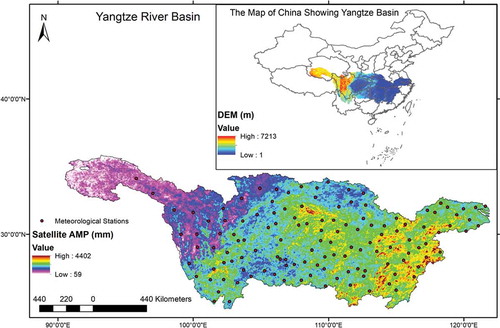
Daily AM data covering 1948–2013 at 128 stations was used for the analysis. The locations of the stations are shown in Fig. 1. The AM series were extracted from the daily datasets obtained from the National Meteorological Information Center of China Meteorological Administration (http://cdc.cma.gov.cn/index.jsp). The associated elevation values for the gauging stations were available along with the datasets. The quality of the datasets is ensured by the same organization. In this study, stations having data lengths greater than 50 years were used. The higher data length ensures the standard error of the estimate will be at the minimum level, which allows the outcome to be robust. The average length of the data series is about 57 years.

The satellite value of AMP was derived from the Tropical Rainfall Measuring Mission (TRMM), a joint mission between NASA and the Japan Aerospace Exploration Agency designed to monitor and study tropical rainfall. The AMP values were obtained from the compilation by Bookhagen (2013) which is based on a 12-year time series of the TRMM 2B31 product. The values are shown in Fig. 1 in map format.

3 Methodology

3.1 Site-specific pooling group and the associated evaluation tool

The ultimate goal of a frequency analysis is to estimate return period values at a study location. Regional analysis in terms of site-specific pooling offers a unique way to group sites for a specific location in an area. The approach uses the ROI method (Burn 1990) to pick stations that are hydrometeorologically similar in terms of the similarity distance measure. The method is generally formulated to avoid conflicts at the boundaries of regions associated with the traditional regional methods. Thus, the primary difference from the traditional (fixed-region) method lies in the technique that assists in forming groups. The homogeneity assessment and the frequency analysis are conducted in a similar way to how they are carried out in the traditional method.

The formation of homogeneous groups with the ROI method depends primarily on two criteria: selection of appropriate site descriptors in the similarity distance measure and the group size. Upon formation of a group, its homogeneity is assessed by a heterogeneity check. The Euclidean distance, $d_{ij}$ (Institute of Hydrology 1999), in the site descriptor space is generally used to estimate the similarity between the target ($i^{th}$) and pooled ($j^{th}$) sites. The general form of the Euclidean distance measure is as follows:

(1) $d_{ij}=\sqrt{{\sum }_{k=1}^n{W}_k{\left(X_{k,i}-X_{k,j}\right)}^2}$(1)

where $n$ is the number of descriptors; $X_{k,i}$and $X_{k,j}$ are the values of the $k^{th}$ descriptor at the $i^{th}$ and$j^{th}$ site, respectively; and $W_k$ is the weight allotted to the descriptors.

In this study, $W_k$ is taken as 1 (when a set comprises more than one descriptor) following the recommendation by Hosking and Wallis (1997, p. 147): when “choosing an appropriate weight is difficult and … the problem is analogous to that of deciding appropriate weights to assign to the variables used in a cluster analysis.” A similar observation was made by Bobée and Rasmussen (1995): “the selection and weighting of variables is one of the problems where no strict mathematical solution is available, but use of common sense can lead to quite acceptable results.”

The geographical and climatological descriptors are widely used in the calculation of $d_{ij}$. However, an assessment is required to find a suitable combination of descriptors so that a robust ROI model can be achieved that can even be implemented in ungauged cases. In terms of pooling group size, the 5T rule (Institute of Hydrology 1999) is often employed; this refers to the total number of station-years of data to be included when estimating the T-year event. However, a group containing 500 station-years produced a good performance (in terms of minimizing error) for a range of recurrence levels up to 100 years (Kjeldsen et al. 2008).

The groups so formed are then assessed with a homogeneity test. The popular and powerful heterogeneity measure, $H_1$, by Hosking and Wallis (1997), is used to testify the homogeneity of a group. The test, which is based on the L-coefficient of variation (L-CV), computes the sample variability of L-CV among the samples in the group and compares it to the variation that would be expected in a homogeneous group. The variability is defined as

(2) $V_1={\left[{\sum }_{i=1}^M{n}_i{\left(t_2^i-t_2^R\right)}^2/{\sum }_{i=1}^M{n}_i\right]}^{1/2}$(2)

where $t_2^i$ and $n_i$ are the values of L-CV and the sample size for site$i$; $M$ is the number of sites in the group and $t_2^R$ is the group average of L-CV.

The expected value ($\mu {\upsilon }_1$) and the standard deviation ($\sigma {\upsilon }_1$) of $V_1$for a homogeneous group are obtained by simulation. Homogeneous groups in large numbers were generated using the four-parameter distribution, kappa, with L-moment ratio values equal to $t_2^R$, $t_3^R$and $t_4^R$and the at-site mean (L-moment 1) equal to 1. The following equation is then used to estimate $H_1$:

(3) $H_1=\frac{\left(V_1-\mu {\upsilon }_1\right)}{\sigma {\upsilon }_1}$(3)

According to the guideline set by Hosking and Wallis (1997), a region is considered to be “acceptably homogeneous” if $H_1<1$, “possibly heterogeneous” if $1<H_1<2$, and “definitely heterogeneous” if $H_1>2$.

3.2 Estimation of return period values

The regional frequency procedure including the ROI framework uses the index-flood method (Dalrymple 1960) to estimate return period values. With this method, a regional/pooled growth curve ($X_T$) in terms of return period ($T$) is calculated that is common to all scaled data recorded at all sites within a homogeneous region/group. The regional curve is then multiplied by the at-site index value $(P_{Index,j})$ to obtain the estimate of quantile $P_{T,j}$ for site (Hosking and Wallis 1997, Institute of Hydrology 1999):

(4) $P_{T,j}=P_{Index,j}\cdot X_T$(4)

The mean or median of the subject site’s AM series is generally taken as the index measurement. This study uses median value as the index measurement because it is unaffected by the presence of outliers (Institute of Hydrology 1999).

The estimation of growth curve requires the identification of a suitable distribution. There are several ways to determine the suitability of a distribution. The L-moment ratio diagram (LMRD) (Vogel and Fennessey 1993, Hosking and Wallis 1997) and Hosking-Wallis goodness-of-fit (GOF) measure (Hosking and Wallis 1997) are two popular methods. The latter approach is applicable to pooling groups that are not identified in the first place in this work; in fact, this is one of the aims of this study: to produce an appropriate ROI grouping scheme. Hence, LMRD is applied to identify a suitable distribution for the whole study region. Later the groups identified by the selected ROI were assessed by the Hosking-Wallis GOF measure. The GEV (Hosking and Wallis 1997) was found to be a suitable distribution for the study region. The suitability of the GEV is explained in detail in Section 4.1.

The GEV with three parameters, location ($\xi$), scale ($\alpha$) and shape ($\kappa$), defined by (Hosking and Wallis 1997) has the following expression

(5) $F\left(x\right)=e^{-e^{-y}},y=\left\{\begin{array}{c}-k^{-1}log\left\{1-\frac{k\left(x-\xi \right)}{\alpha }\right\},k\ne 0\\ \left(x-\xi \right)/\alpha ,k=0\end{array}\right.$(5)

The shape parameter influences the tail behaviour: for $\kappa =0$, the distribution is two-parameter Gumbel; for k<0, the distribution is lower bounded whereas for k>0, the distribution is upper bounded.

The growth curve (see Equation 4)(4) $P_{T,j}=P_{Index,j}\cdot X_T$(4) based on GEV (reduced to two parameters: $\kappa$ and beta, $\beta$) has the following form (Das and Cunnane 2011):

(6) ${\mathrm{X}}_{\mathrm{T}}=1+\frac{\beta }{\kappa }\left({\left(\mathrm{l}\mathrm{n}2\right)}^{\kappa }-{\left(\mathrm{l}\mathrm{n}\left(\frac{\mathrm{T}}{\mathrm{T}-1}\right)\right)}^{\kappa }\right)$(6)

The parameters estimated based on L-moments (Hosking and Wallis 1997) have the following expressions:

(7) $\kappa =7.8590\mathrm{c}+2.9554{\mathrm{c}}^2\mathrm{i}\mathrm{n}\mathrm{w}\mathrm{h}\mathrm{i}\mathrm{c}\mathrm{h}\mathrm{c}=\frac{2}{3+{\mathrm{t}}_3}-\frac{\mathrm{l}\mathrm{n}2}{\mathrm{l}\mathrm{n}3}$(7)

(8) $\beta =\frac{\kappa {\mathrm{t}}_2}{{\mathrm{t}}_2\left(\mathrm{\Gamma }\left(1+\kappa \right)-{\left(\mathrm{l}\mathrm{n}2\right)}^{\kappa }\right)+\mathrm{\Gamma }\left(1+\kappa \right)\left(1-2^{-\kappa }\right)}$(8)

where $t_2$ is the L-coefficient of variation (L-CV), $t_3$ is the L-skewness and $\mathrm{\Gamma }$ is the complete gamma function.

The regional/pooled estimate of $t_2$ and $t_3$ takes it to the regional/pooled growth curve (Hosking and Wallis 1997). The regional estimate of $t_2$ and $t_3$ can be achieved based on the following equation:

(9) $t^{\left(i\right)R}=\frac{{\sum }_{j=1}^M{w}_{ij}{t}^{\left(j\right)}}{{\sum }_{j=1}^M{w}_{ij}}$(9)

where $t^{\left(j\right)}$ is either $t_2$ or $t_3$ for the $j^{th}$ most analogous site and $w_{ij}$ is a weight, generally taken proportional to the record length.

This study considers $w_{ij}$ to be 1 (unweighted average) following the observation noted by Hosking and Wallis (1997, p. 90): weighting it “proportionally to record length may give undue influence to sites that have frequency distributions markedly different from the region as a whole and that also have long records.”

3.3 ROI models

ROI models differ in their similarity distance measure (see Equation 1)(1) $d_{ij}=\sqrt{{\sum }_{k=1}^n{W}_k{\left(X_{k,i}-X_{k,j}\right)}^2}$(1) . A set of different descriptors (also known as pooling variables) and their combinations are generally tested to find the right one. When selecting, it is kept in mind that the chosen set should be applicable under ungauged conditions. It should also be easily accessible. A suitable ROI model is generally used for the whole region. A range of descriptors, primarily the geographical and climatological descriptors, are commonly used (Gaál and Kyselý 2009, Das 2017). However, the application of remotely sensed data is scarcely carried out.

Four site descriptors are employed in this study. Among them three are geographical (location descriptors in the form of longitude and latitude, and elevation) and one is a climatological descriptor (AMP). The location attributes are selected since the geographical proximity of the sites has proved to deliver favourable results in finding similar regimes of extreme precipitation (Reed et al. 1999, Kyselý et al. 2011, Das 2018, Requena et al. 2019a). The elevation is quite an instinctive choice since it is fairly well correlated with the precipitation field (Goovaerts 2000, Lloyd 2005). The descriptor is routinely used in ROI methodology (Das 2017, Ball et al. 2019). The AMP is also used in delineating successful homogeneous pooling groups (Gaál et al. 2008). Because observed AMP values are only available at gauged locations, the descriptor in this form may not be useful for ungauged cases. This study, thus, takes the satellite-based AMP values. The TRMM-derived AMP value has shown a good relation with the observed AMP in different territories of the world including China (Shi et al. 2015). Therefore, the remotely sensed data such as AMP has the ability to serve as a pooling variable for ROI methodology.

Based on four site descriptors, several different ROI models are formed. In order to make a comparison, in particular, with the remotely sensed AMP, an additional model containing the observed AMP is included. Table 1 lists the details of these models. The weight is taken as 1 (see Equation 1)(1) $d_{ij}=\sqrt{{\sum }_{k=1}^n{W}_k{\left(X_{k,i}-X_{k,j}\right)}^2}$(1) when a set consists of more than one descriptor (see e.g. ROI-5 and ROI-6).

Table 1. Description of ROI models that differ in their similarity distance measure

ROI model	Description
ROI-1	Physical distance: Site descriptors “latitude” and “longitude” are used to calculate the proximity between sites
ROI-2	Elevation
ROI-3	Remotely sensed annual mean precipitation (AMP). The TRMM-based AMP is used so that it can be employed at ungauged locations
ROI-4	Physical distance + Elevation
ROI-5	Physical distance + AMP
ROI-6	Physical distance + Elevation +AMP
ROI-7	Observed AMP

3.4 Means of assessment

3.4.1 Assessment between ROI models

ROI models listed in Table 1 were compared using a simulation framework. The GEV distribution suitable for the study region is used by this framework to generate data. The framework is a two-step procedure. In the first step, at-site population values of $t_2$ and $t_3$ were estimated which were then used to generate data. The use of observed at-site $t_2$ and $t_3$ as population values is considered to yield a simulated region that has much more heterogeneity than the actual data. As a consequence, Hosking and Wallis (1997, p. 93) recommended not using the observed at-site L-moment ratio values for simulation purposes. In the second step, the core simulation was conducted.

The present study uses a method outlined by Das and Cunnane (2011) to estimate at-site population values of $t_2$ and $t_3$. A similar approach can be found in other ROI studies (e.g. Castellarin et al. 2001, Gaál et al. 2008). The method uses a ROI approach with a distance measure (${\delta }_{i,j}$) defined in Equation (10)(10) ${\delta }_{i,j}=\sqrt{{\left(\frac{t_{2,i}-t_{2,j}}{{\sigma }_{t_2}}\right)}^2+{\left(\frac{t_{3,i}-t_{3,j}}{{\sigma }_{t_3}}\right)}^2}$(10) to form a group for a subject site. The population values of $t_2$ and $t_3$ are then appraised as the resultant pooled estimate of $t_2$ and $t_3$ using Equation (9)(9) $t^{\left(i\right)R}=\frac{{\sum }_{j=1}^M{w}_{ij}{t}^{\left(j\right)}}{{\sum }_{j=1}^M{w}_{ij}}$(9) .

(10) ${\delta }_{i,j}=\sqrt{{\left(\frac{t_{2,i}-t_{2,j}}{{\sigma }_{t_2}}\right)}^2+{\left(\frac{t_{3,i}-t_{3,j}}{{\sigma }_{t_3}}\right)}^2}$(10)

In the core simulation, the random series for each site was generated based on GEV with L-moments equal to the at-site population values of $t_2$ and $t_3$ (estimated in first step). The $X_T$ value for a target site (a pooling group is formed for the target site) was then evaluated using Equation (6)(6) ${\mathrm{X}}_{\mathrm{T}}=1+\frac{\beta }{\kappa }\left({\left(\mathrm{l}\mathrm{n}2\right)}^{\kappa }-{\left(\mathrm{l}\mathrm{n}\left(\frac{\mathrm{T}}{\mathrm{T}-1}\right)\right)}^{\kappa }\right)$(6) following the estimation of $\kappa$ and $\beta$ using Equations (7(7) $\kappa =7.8590\mathrm{c}+2.9554{\mathrm{c}}^2\mathrm{i}\mathrm{n}\mathrm{w}\mathrm{h}\mathrm{i}\mathrm{c}\mathrm{h}\mathrm{c}=\frac{2}{3+{\mathrm{t}}_3}-\frac{\mathrm{l}\mathrm{n}2}{\mathrm{l}\mathrm{n}3}$(7) –8(8) $\beta =\frac{\kappa {\mathrm{t}}_2}{{\mathrm{t}}_2\left(\mathrm{\Gamma }\left(1+\kappa \right)-{\left(\mathrm{l}\mathrm{n}2\right)}^{\kappa }\right)+\mathrm{\Gamma }\left(1+\kappa \right)\left(1-2^{-\kappa }\right)}$(8) ) based on the pooled estimate of $t_2$ and $t_3$ values. A detailed description of the simulation procedure can be obtained from Das and Cunnane (2011). The root mean square error ($RMS{E}_T$), defined in Equation (11(11) $RMS{E}_T=\frac{1}{M}{\sum }_{i=1}^M\sqrt{\frac{1}{R}{\sum }_{r=1}^R{\left(\frac{{\hat{X}}_{i,r}^T-X_i^T}{X_i^T}\right)}^2}$(11) ), was then employed to compare ROI models.

(11) $RMS{E}_T=\frac{1}{M}{\sum }_{i=1}^M\sqrt{\frac{1}{R}{\sum }_{r=1}^R{\left(\frac{{\hat{X}}_{i,r}^T-X_i^T}{X_i^T}\right)}^2}$(11)

where ${\hat{X}}_{i,r}^T$ is the estimated $T$-year pooled growth factor at site $i$ at the $r^{th}$ repetition, $X_i^T$ is the true $T$-year growth factor at site $i$, $M$is the total number of group members and $R$is the total number of repetitions (10 000 used in this study).

3.4.2 Assessment of ROI and regional models

The pooled uncertainty measure (PUM) was used to compare between the selected ROI model and the regional models. Simulated data (such as the synthetic data generation presented in an earlier section) was not used; rather, the actual data was used in the comparison because the models were already identified. The PUM for the return period , defined by the Flood Estimation Handbook (Institute of Hydrology 1999), is a form of weighted average of the differences between each site growth factor and the pooled growth factor measured on a logarithmic scale:

(12) $PU{M}_T=\sqrt{\frac{{\sum }_{i=1}^{M_{long}}{n}_i\left(ln{X}_{T_i}-ln{X}_T^P\right)}{{\sum }_{i=1}^{M_{long}}{n}_i}}$(12)

where $M_{long}$ is the number of long-record sites in a group, $n$is the record length, $X_{T_i}$ is the T-year site growth factor at the $i^{th}$ site and $X_T^P$ is the T-year pooled growth factor. In this study, stations that have a record length of over 50 years were used. Thus, all sites in a group are considered $M_{long}$.

4 Results and analysis

4.1 Distribution selection

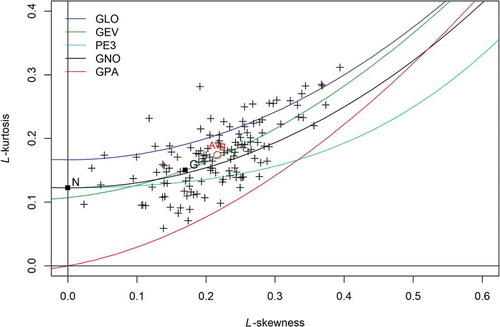
The choice of distribution plays a pivotal role in frequency analysis. In this study the distribution is identified using the LMRD. The AM series were analysed using the diagram; this analysis is reported in Fig. 2. The average estimation of L-moment ratio value falls on the theoretical line of GEV, which signifies that GEV is the most appropriate distribution for the Yangtze basin. Thus, GEV is considered to be the characteristic distribution for carrying out precipitation frequency analysis.

Figure 2. Distribution selection by the L-moment ratio diagram. Three-parameter candidate distributions are represented by lines: GLO, generalized logistic; GEV, generalized extreme value; PE3, Pearson Type III; GNO, generalized normal; GPA, generalized Pareto. Two-parameter distributions are represented by points: N, normal; G, Gumbel. The average value of L-moment ratio (red circle) falls on the GEV line

4.2 ROI model selection

The simulation framework (see Section 3.4.1) that generates samples under GEV distribution was used to compare the considered ROI models. The error measure in the form of RMSE_T defined in Equation (11(11) $RMS{E}_T=\frac{1}{M}{\sum }_{i=1}^M\sqrt{\frac{1}{R}{\sum }_{r=1}^R{\left(\frac{{\hat{X}}_{i,r}^T-X_i^T}{X_i^T}\right)}^2}$(11) ) was assessed at return periods of 10, 50 and 100 years for each station. Data from 128 stations were used in the assessment which, in turn, produces with the ROI approach 128 pooling groups.

The variation in RMSE values at the target return levels is displayed in box plot form for different schemes in Fig. 3. The associated average values are tabulated in Table 2. It appears that the statistic differs by a very small number between ROI schemes. The set that encompasses physical distance and elevation (ROI-4) performed best in connection with providing the smallest RMSE100 value, while the set consisting of only remotely sensed AMP (ROI-3) came last in the list. The set consisting of all variables (ROI-6) achieved an error comparable to that of ROI-4 but was not superior to the ROI-4 model. The same outcome is also obtained for the small and mid-range return period context: RMSE10 and RMSE 50. The observed AMP was included to compare its performance against the ROI schemes, in particular against ROI-3. That scheme (ROI-7) performed better than ROI-3 but could not outperform ROI-4, the selected model.

Table 2. Comparison of results in terms of mean RMSE corresponding to T = 10, 50 and 100 years for different ROI models listed in Table 1

Models	RMSE10	RMSE50	RMSE100
ROI-1	0.0529	0.1087	0.1347
ROI-2	0.0508	0.1057	0.1313
ROI-3	0.0602	0.1214	0.1495
ROI-4	0.0472	0.1003	0.1255
ROI-5	0.0530	0.1092	0.1356
ROI-6	0.0473	0.1004	0.1257
ROI-7	0.0589	0.1182	0.1453

Figure 3. Assessment of different ROI models. RMSE values in box plot format in three return periods (10, 50 and 100 years) are evaluated. Each box plot contains 128 values

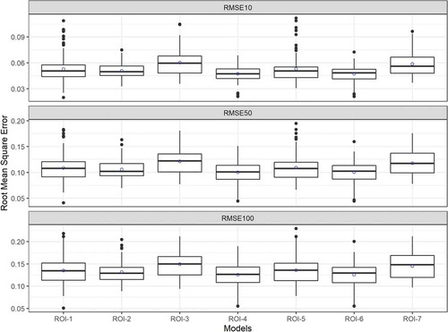
In general, the geographical distance and elevation can be taken as being the most appropriate pooling variables for Yangtze basin, and this combination performed better than the attributes associated with remotely sensed data.

4.3 Comparison between site-specific ROI model and regional model

The ROI-4 model is identified as the most appropriate site-specific pooling model for Yangtze basin. The model is compared against the regional models that have been successfully applied to the basin.

Two regional models were taken into consideration for comparison. One is based on a study by Chen et al. (2013) and is labelled R-I. Six homogeneous regions were identified using the fuzzy c-mean clustering methodology. The second one comprises 11 hydrological sub-basins divided over the whole basin. These sub-basins were used as regions in conducting a regional frequency analysis (Su et al. 2008, 2009). This model is termed R-II. The delineated regions are shown in both cases with the current datasets in Fig. 4.

Figure 4. Regions by R-I and R-II models with current datasets. R-I was delineated by cluster analysis (Chen et al. 2013) while R-II was delineated based on sub-basins (Su et al. 2009)

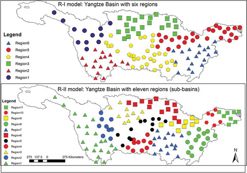
The homogeneity criterion is an important condition for a successful regional analysis. However, several studies identified that a weak homogeneity still should be more considered effective for estimating high return period values than conducting at-site frequency analysis (Hosking and Wallis 1997, Institute of Hydrology 1999). With the current datasets, the homogeneity test was revisited for both regional models. The heterogeneity measure quantified for both models is reported in Table 3. All the regions in R-I are judged to be homogeneous, which is not surprising considering that they were homogeneously delineated in the previous study. Thus, the regions formed by Chen et al. (2013) are deemed robust considering that a little variation in the datasets does not affect the homogeneity of the regions. On the other hand, mixed results were identified with R-II. Out of 11 regions, three are heterogeneous and eight are homogeneous. All of the heterogeneous regions belong to the Upper Yangtze basin. In the case of the ROI model, over 91% of the groups are homogeneous.

Table 3. Heterogeneity measure, H1 and PUM value in three return periods for regions delineated by the regional models with current datasets

Region (Model-I)	H1	PUM10	PUM50	PUM100
R-I: 1	0.58	0.0319	0.0642	0.0795
R-I: 2	1.5	0.057	0.1096	0.1351
R-I: 3	0.9	0.0606	0.1227	0.1521
R-I: 4	0.25	0.0541	0.1175	0.1482
R-I: 5	−0.14	0.06	0.135	0.1712
R-I: 6	0.26	0.0523	0.1089	0.137
Regions (Model-II)	H1	PUM10	PUM50	PUM100
R-II: 1	5.6	0.0746	0.1445	0.1761
R-II: 2	5.3	0.1047	0.1817	0.213
R-II: 3	4.8	0.0944	0.1702	0.2018
R-II: 4	−0.18	0.0493	0.1176	0.152
R-II: 5	−0.84	0.0427	0.0972	0.1245
R-II: 6	0.81	0.0608	0.1146	0.1393
R-II: 7	1.26	0.0646	0.1363	0.1698
R-II: 8	1.11	0.0572	0.115	0.1435
R-II: 9	0.175	0.0591	0.1313	0.1665
R-II: 10	0.468	0.0676	0.1421	0.1785
R-II: 11	0.014	0.0581	0.1315	0.1682

The homogeneity measure is like a significance test (Hosking and Wallis 1997), thus being homogeneous does not guarantee a superior model. Hence, an error measure is needed. The PUM described in Section 3.4.2 was used to compare two different categories of models. The PUM values measured at T = 10, 50, 100 are displayed in box plots in Fig. 5. Six data points, 11 data points and 128 data points were used to construct box plots for R-I, R-II and ROI-4, respectively. The PUM value in an individual case is reported in Table 3 (only for R-I and R-II) to demonstrate how a heterogeneous region leads to a higher quantity of error. The variation in the mean PUM value between models is reported in Table 4. It appears that the statistic differs by a very small amount between the models. The ROI model has the lowest PUM value, followed by R-I and R-II, in the three representative return period contexts: lower ($X_{10}$) as well as medium ($X_{50}$) and higher growth factors ($X_{100}$).

Table 4. Summary comparison results between site-specific, ROI-4 and regional models: R-I and R-II in terms of mean PUM value

Models	Mean PUM10	Mean PUM50	Mean PUM100
R-I	0.0527	0.1097	0.1372
R-II	0.0666	0.1347	0.1667
ROI-4	0.0521	0.1083	0.1352

Figure 5. Model selection based on PUM value in box plot form in three return periods: 10, 50 and 100 years. R-I contains six values, R-II contains 11 values and ROI-4 contains 128 values

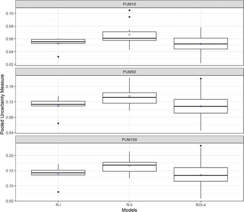
The regional model consisting of 11 hydrological sub-basins (R-II) is the least suitable method for the estimation of daily extreme precipitation quantiles. The reason might be the effect of three heterogeneous regions which greatly contributed to the overall PUM value. Although the R-I model performed better than R-II, the homogeneously formed regions were unable to outperform the ROI model in terms of mean PUM value. The difference in error between them is, however, not very large. The superior performance of ROI-4 and R-I over R-II suggests that the improved methods with additional variables give rise to a significant difference in PUM value. While R-I uses a clustering technique to divide a large group of datasets into several smaller groups, ROI selects a tailor-made group of stations for a subject site. In both cases, the similarity is provided by the chosen descriptors. In general, the identified ROI model is able to reduce the error and leads to more reliable extreme precipitation estimates over the Yangtze River basin.

5 Discussion

The accomplishments of the selected model (ROI-4) are further discussed in this section. The first point of discussion is the selection of site descriptors. Although the inclusion of remotely sensed data provides a new direction for the ROI regional analysis, the inclusion is unable to outperform the traditional (geographic) at-site observed descriptors. The location information and elevation that were identified as suitable in the distance measure are easily accessible and could be used to delineate groups for ungauged conditions. The identification of close proximity as an effective descriptor is no surprise as the regional analysis itself is based on the idea that nearby stations in a region possess similar hydroclimatological characteristics. Close proximity was found to deliver successful results in several past ROI studies (Das 2018, Requena et al. 2019a).

The addition of elevation further improves the accuracy of the model. Elevation/altitude is relatively high in the western part of the basin (upper basin) but drops dramatically towards the east. The systematic drop helps to group the stations appropriately in the study area. As a result, the inclusion of physical distance and elevation combined in the similarity distance measure serves a major role in characterizing the behaviour of extreme precipitation. The analogous distance measure defined in three dimensions using latitude, longitude and elevation was also found suitable in Australian context (Johnson and Green 2018, Ball et al. 2019). The results regarding geographic descriptors displaying superior performance to climatic descriptors are consistent with the findings of Johnson and Green (2018).

Although the incorporation of remotely sensed data was unable to overpower the traditional attributes in terms of error, the introduction of remotely sensed data paves a new way to be used with the ROI method. Due to the advent of space technology, remotely sensed data are available, but they are hardly used in regional frequency analysis. Future studies should explore their application in other basins around the world. There is an intuitive appeal to using this approach in countries where the density of gauged stations is low or where there are difficulties in installing meteorological stations.

Considering the importance of selecting a suitable distribution in the frequency analysis, we revisit our distribution selection with the selected model. The ROI-4 model is applied to each site and a pooling group is formed with a minimum of 500 years of data. The Hosking-Wallis GOF is applied to each pooling group. The GEV was the best distribution for 63% of cases and was acceptable in 100% of cases. The second best GNO was acceptable for 90% of sites but was the best distribution in only 26% of cases. The performance was sub-par for the remaining three distributions: GLO, PE3 and GPA. Thus, the GEV provided the best overall fit to the AM data of Yangtze basin. This supported the initial selection by the LMRD. The selection is also consistent with the findings of Chen et al. (2013) for the same basin.

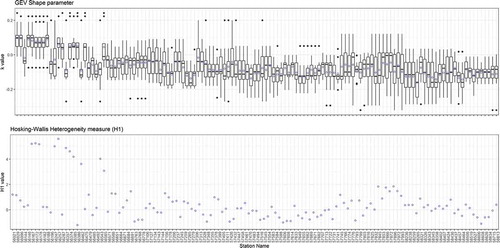
Further insights were explored for groups formed based on the selected model. Two statistics were examined that are critical to frequency analysis: the heterogeneity measure and the shape parameter of the GEV distribution. They reveal the deep understanding of the model in evaluating extreme precipitation.

The variation of the shape parameter ($\kappa$) and the corresponding pooled average $\kappa$ value, indicated by a circle, is displayed in box plot form in Fig. 6. The ${\mathrm{H}}_1$ value evaluated for each group is also displayed in the same figure. Most of the pooling groups (over 91%) passed the homogeneity test, with ${\mathrm{H}}_1$ values of less than 2. This justifies the use of combined descriptors: physical distance and elevation as pooling variables. The shape parameter, which plays a pivotal role in describing the tail behaviour of the distribution, is effectively scaled down by the ROI methodology. Similar characteristics were also noticed by Johnson and Green (2018) in their study. The pooled (group average) value of the shape parameter of most pooling groups (about 90%) is below zero which suggests that the model is unbounded (see the parametrization of GEV in Section 3.2). The use of this unbounded condition is often advisable in engineering practice (Papalexiou and Koutsoyiannis 2013) as it yields increasing difference in design precipitation between high recurrence intervals.

Figure 6. Shape parameter (k) value and heterogeneity measure of pooling groups delineated by ROI-4 model for each station. Group members’ shape parameter values are shown in box plot form with the pooled average indicated with blue circles

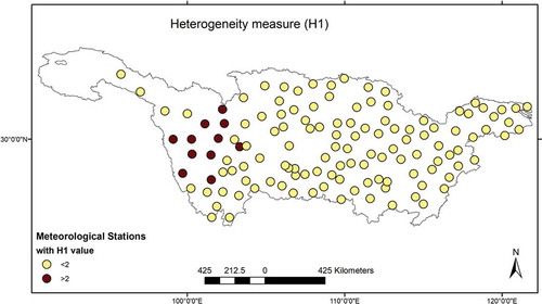
It is interesting to note that in several cases the upper bounded condition is correlated with the non-homogeneity of the group, as can be seen from Fig. 6. Another aspect to point out is that all the heterogeneous groups belong to the upper basin (see Fig. 7). A possible reason is that these stations are located in the upper part of the basin, a distinct climatic area, where fewer meteorological stations are available. This permits the model to use a number of stations from other regions to complete the 500 station-year dataset (about 10 stations per group), which may bring heterogeneity into the groups. In addition, the extremes and the yearly variation of AM data are not that significantly high, which may induce an upper bounded condition. It is suggested to carefully check ROI groups formed in this area and, if necessary, to refine the group members manually as per the suggestion by Hosking and Wallis (1997).

Figure 7. Spatial distribution of the heterogeneity measure (H1) for groups delineated based on the ROI-4 model at the gauged sites

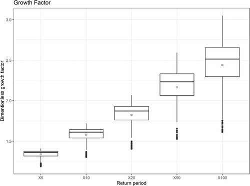
Finally, the growth factor estimated by the selected model is also assessed. The growth factors estimated for each pooling group are presented in box plots with respect to return periods in Fig. 8. A box plot for a particular return period includes the corresponding values for all stations. The mean value increases with an increasing return periods, which is understandable considering that the model, in most cases, is unbounded. The range in each case also provides a sense of uncertainty regarding how the growth factor (e.g. design estimation) can vary within a specified return period.

Figure 8. Box plots of growth factors with respect to return period. Each box plot contains values for all stations (pooling group formed for each station)

6 Conclusion

This study compares two types of at-site attributes, observed and remotely sensed, to include in the site-specific pooling approach in the estimation of extreme precipitation. The study also examines whether the selected site-specific regional model is superior to the traditional regional group in conducting regional precipitation frequency analysis in Chinese climatic conditions. The present work is carried out in Yangtze basin which is deemed appropriate for performing such examinations considering its gigantic size with varying climatic and topographical regions.

Regarding the first objective, a combination of descriptors – location variables (latitude and longitude), elevation and remotely sensed annual mean precipitation – was used. The satellite data is employed so that if selected, the attribute can be applied at ungauged locations similar to other descriptors considered. Several ROI models that differ in their similarity distance measure were investigated. With respect to the second objective, two regional models (one based on a geographical approach and the other based on a clustering approach) were examined relative to the selected ROI model.

Annual maximum daily precipitation data from 128 stations were analysed to assess the study. Only stations with a high record length (N >50) were considered for the analysis. The first aim was evaluated using a simulation technique in which data were generated based on the representative GEV distribution. The second aim was assessed using an uncertainty measure, namely PUM, based on observed data.

From the study, we draw the following conclusions:

• The GEV provided the best overall fit to the annual maximum precipitation data of the Yangtze basin.

• Although the inclusion of remotely sensed data provides a new direction for the ROI regional analysis, its incorporation was unable to outperform the traditional observed site descriptors. The ROI scheme based on physical distance and elevation combined attained the best results among the considered schemes. The groups delineated by the model in most cases successfully passed the homogeneity test. This indicates that the identified similarity measure has a strong link with the governing character of extreme precipitation in the study area. Barring a few instances, the frequency behaviour in most cases is unbounded, which is attractive in practical applications.

• The ROI, which allows having a tailor-made pooling group for a target site, was found to be superior to the traditional regional models examined in this study. The regional model that divides the whole basin into 11 sub-basins was identified as the least appropriate for estimating extreme precipitation, while the model that used a clustering technique to divide the basin into six homogeneous regions was found to be very close to the ROI model in terms of error measure.

The study is expected to help engineers and water resource managers to assess flood risk in the study region. Although the inclusion of remotely sensed data was outperformed in this case study, future studies should explore its application in other basins across the world. Further research is also required to refine the group selection criteria for the assessment of the ROI approach in the upper part of the Yangtze basin.

Acknowledgements

The authors thank Ana Requena (Associate Editor), Saeid Eslamian and one anonymous reviewer for their critical comments, which helped improve the quality of the manuscript.

Disclosure statement

No potential conflict of interest was reported by the authors.

Additional information

Funding

The study was funded by the NUIST faculty start-up grant [grant number 2243141501015] to the first author. Daily precipitation data series were obtained from the National Meteorological Information Center of China Meteorological Administration. The data that support the findings of this study are available on request from the corresponding author. The data are not publicly available due to privacy or ethical restrictions.

References

- Ball, J., Babister, M., Nathan, R., Weeks, W., Weinmann, E., Retallick, M. and Testoni, I., (Editors), 2019. Australian rainfall and runoff: a guide to flood estimation, © Commonwealth of Australia (Geoscience Australia). Barton, ACT, 1–199.
- Bobée, B. and Rasmussen, P.F., 1995. Recent advances in flood frequency analysis. Reviews of Geophysics, 33(S2), 1111–1116, doi:https://doi.org/10.1029/95RG00287, John Wiley & Sons, Ltd.
- Bookhagen, B. (2013) High resolution spatiotemporal distribution of rainfall seasonality and extreme events based on a 12-year TRMM time series. Available from: http://www.geog.ucsb.edu/~bodo/TRMM/index.php [Accessed 05 December 2020].
- Burn, D.H., 1990. Evaluation of regional flood frequency analysis with a region of influence approach. Water Resources Research, 26 (10), 2257–2265. Wiley Online Library. doi:https://doi.org/10.1029/WR026i010p02257.
- Castellarin, A., Burn, D., and Brath, A., 2001. Assessing the effectiveness of hydrological similarity measures for flood frequency analysis. Journal of Hydrology, 241 (3–4), 270–285. doi:https://doi.org/10.1016/S0022-1694(00)00383-8
- Chen, Y.D., et al., 2013. Precipitation extremes in the Yangtze River Basin, China: regional frequency and spatial–temporal patterns. Theoretical and Applied Climatology, 116 (3–4), 447–461. doi:https://doi.org/10.1007/s00704-013-0964-3
- Cunnane, C., 1988. Methods and merits of regional flood frequency analysis. Journal of Hydrology, 100, 269–290. doi:https://doi.org/10.1016/0022-1694(88)90188-6
- Dalrymple, T., 1960. Flood frequency methods. Vol. 1543–A. Reston: U. S. Geol. Surv, 11–51.
- Darwish, M.M., et al., 2020. New hourly extreme precipitation regions and regional annual probability estimates for the UK. International Journal of Climatology. April, 1–19. doi:https://doi.org/10.1002/joc.6639
- Das, S., 2017. Performance of region-of-influence approach of frequency analysis of extreme rainfall in monsoon climate conditions. International Journal of Climatology, 37, 612–623. doi:https://doi.org/10.1002/joc.5025
- Das, S., 2018. Extreme rainfall estimation at ungauged sites: comparison between region‐of‐influence approach of regional analysis and spatial interpolation technique. International Journal of Climatology. July, 1–17. doi:https://doi.org/10.1002/JOC.5819
- Das, S., 2021. Extreme rainfall estimation at ungauged locations: information that needs to be included in low-lying monsoon climate regions like Bangladesh. Journal of Hydrology, 601, 126616. doi:https://doi.org/10.1016/j.jhydrol.2021.126616
- Das, S. and Cunnane, C., 2011. Examination of homogeneity of selected Irish pooling groups. Hydrology and Earth System Sciences, 15 (3), 819–830. doi:https://doi.org/10.5194/hess-15-819-2011
- Das, S., Zhu, D., and Yin, Y., 2020. Comparison of mapping approaches for estimating extreme precipitation of any return period at ungauged locations. Stochastic Environmental Research and Risk Assessment, Springer Berlin Heidelberg 7. https://doi.org/10.1007/s00477-020-01828-7.
- Dehghan, Z., et al., 2019. Regional frequency analysis with development of region-of-influence approach for maximum 24-h rainfall (case study: urmia Lake Basin, Iran). Theoretical and Applied Climatology, 136 (3–4), 1483–1494. doi:https://doi.org/10.1007/s00704-018-2574-6
- Eslamian, S.S., 1995. Regional flood frequency analysis using a region of influence’approach. Sydney, Australia: University of New South Wales.
- Fang, B., et al., 2007. Non-identical models for seasonal flood frequency analysis. Hydrological Sciences Journal, 52 (5), 974–991. doi:https://doi.org/10.1623/hysj.52.5.974
- Fowler, H.J. and Kilsby, C.G., 2003. A regional frequency analysis of United Kingdom extreme rainfall from 1961 to 2000. International Journal of Climatology, 23 (11), 1313–1334. doi:https://doi.org/10.1002/joc.943
- Gaál, L. and Kyselý, J., 2009. Comparison of region-of-influence methods for estimating high quantiles of precipitation in a dense dataset in the Czech Republic. Hydrology and Earth System Sciences, 13 (11), 2203–2219. doi:https://doi.org/10.5194/hess-13-2203-2009
- Gaál, L., Kyselý, J., and Szolgay, J., 2008. Region-of-influence approach to a frequency analysis of heavy precipitation in Slovakia. Hydrology and Earth System Sciences, 12 (3), 825–839. doi:https://doi.org/10.5194/hess-12-825-2008
- Gado, T.A., Hsu, K., and Sorooshian, S., 2017. Rainfall frequency analysis for ungauged sites using satellite precipitation products. Journal of Hydrology, 554, 646–655. doi:https://doi.org/10.1016/j.jhydrol.2017.09.043
- Gellens, D., 2002. Combining regional approach and data extension procedure for assessing GEV distribution of extreme precipitation in Belgium. Journal of Hydrology, 268 (1–4), 113–126. doi:https://doi.org/10.1016/S0022-1694(02)00160-9
- Goovaerts, P., 2000. Geostatistical approaches for incorporating elevation into the spatial interpolation of rainfall. Journal of Hydrology, 228, 113–129. doi:https://doi.org/10.1016/S0022-1694(00)00144-X
- Hailegeorgis, T.T., Thorolfsson, S.T., and Alfredsen, K., 2013. Regional frequency analysis of extreme precipitation with consideration of uncertainties to update IDF curves for the city of Trondheim. Journal of Hydrology, 498, 305–318. doi:https://doi.org/10.1016/j.jhydrol.2013.06.019 Elsevier B.V.
- Hosking, J.R.M. and Wallis, J.R., 1997. Regional frequency analysis: an approach based on L-moments. Cambridge: Cambridge University Press.
- Institute of Hydrology., 1999. Flood Estimation Handbook, Vols. 1-5. Wallingford Wallingford, U.K.: Institute of Hydrology.
- Johnson, F. and Green, J., 2018. A comprehensive continent-wide regionalisation investigation for daily design rainfall. Journal of Hydrology: Regional Studies, 16(March), 67–79, doi:https://doi.org/10.1016/j.ejrh.2018.03.001, Elsevier
- Ju, Q., et al., 2014. Response of hydrologic processes to future climate changes in the Yangtze River Basin. Journal of Hydrologic Engineering, 211–222. January. doi:https://doi.org/10.1061/(ASCE)HE.1943-5584.0000770
- Kjeldsen, T., et al.(2008) Improving the FEH statistical method. Flood and Coastal Management Conference 2008. Manchester, UK: University of Manchester: Environment Agency/Defra.
- Kyselý, J., Gaál, L., and Picek, J., 2011. Comparison of regional and at-site approaches to modelling probabilities of heavy precipitation. International Journal of Climatology, 31 (10), 1457–1472. doi:https://doi.org/10.1002/joc.2182
- Lloyd, C.D., 2005. Assessing the effect of integrating elevation data into the estimation of monthly precipitation in Great Britain. Journal of Hydrology, 308 (1), 128–150. doi:https://doi.org/10.1016/j.jhydrol.2004.10.026
- NERC, 1975. Flood studies report. London, U.K: Natural Environment Research Council.
- Norbiato, D., et al., 2007. Regional frequency analysis of extreme precipitation in the eastern Italian Alps and the August 29, 2003 flash flood. Journal of Hydrology, 345 (3–4), 149–166. doi:https://doi.org/10.1016/j.jhydrol.2007.07.009
- Papalexiou, S.M. and Koutsoyiannis, D., 2013. Battle of extreme value distributions: a global survey on extreme daily rainfall. Water Resources Research, 49 (1), 187–201. doi:https://doi.org/10.1029/2012WR012557
- Reed, D.W., Faulkner, D.S., and Stewart, E.J., 1999. The FORGEX method of rainfall growth estimation II: description. Hydrology and Earth Systems Sciences, 3 (2), 197–203. doi:https://doi.org/10.5194/hess-3-205-1999
- Requena, A.I., Burn, D.H., and Coulibaly, P. 2019a. Estimates of gridded relative changes in 24-h extreme rainfall intensities based on pooled frequency analysis. Journal of Hydrology, 577, July. 123940. Elsevier. https://doi.org/10.1016/j.jhydrol.2019.123940
- Requena, A.I., Burn, D.H., and Coulibaly, P., 2019b. Pooled frequency analysis for intensity–duration–frequency curve estimation. Hydrological Processes, 33 (15), 2080–2094. doi:https://doi.org/10.1002/hyp.13456
- Satyanarayana, P. and Srinivas, V.V., 2008. Regional frequency analysis of precipitation using large-scale atmospheric variables. Journal of Geophysical Research Atmospheres, 113 (24), 1–16. doi:https://doi.org/10.1029/2008JD010412
- Shi, Y., et al., 2015. Mapping annual precipitation across Mainland China in the period 2001-2010 from TRMM3B43 product using spatial downscaling approach. Remote Sensing, 7 (5), 5849–5878. doi:https://doi.org/10.3390/rs70505849
- Srivastava, A., et al. 2019. A unified approach to evaluating precipitation frequency estimates with uncertainty quantification: application to Florida and California watersheds. Journal of Hydrology, 578, March. 124095. Elsevier. doi:https://doi.org/10.1016/j.jhydrol.2019.124095
- Su, B., Gemmer, M., and Jiang, T., 2008. Spatial and temporal variation of extreme precipitation over the Yangtze River Basin. Quaternary International, 186 (1), 22–31. doi:https://doi.org/10.1016/j.quaint.2007.09.001
- Su, B., Kundzewicz, Z.W., and Jiang, T., 2009. Simulation of extreme precipitation over the Yangtze River Basin using Wakeby distribution. Theoretical and Applied Climatology, 96, 209–219. doi:https://doi.org/10.1007/s00704-008-0025-5
- Sun, H., et al., 2017. Regional frequency analysis of observed sub-daily rainfall maxima over eastern China. Advances in Atmospheric Sciences, 34 (2), 209–225. doi:https://doi.org/10.1007/s00376-016-6086-y
- Svensson, C. and Jones, D.A., 2010. Review of rainfall frequency estimation methods. Journal of Flood Risk Management, 3 (4), 296–313. doi:https://doi.org/10.1111/j.1753-318X.2010.01079.x/abstract
- Viglione, A., Laio, F., and Claps, P., 2007. A comparison of homogeneity tests for regional frequency analysis Wiley Online Library. Water Resources Research - WATER RESOUR RES, 43 (3). doi: https://doi.org/10.1029/2006WR005095
- Vogel, R.M. and Fennessey, N.M., 1993. L moment diagrams should replace product moment diagrams. Water Resources Research, 29 (6), 1745–1752. Wiley Online Library. https://doi.org/10.1029/93WR00341.
- Wagner, P.D., et al., 2012. Comparison and evaluation of spatial interpolation schemes for daily rainfall in data scarce regions. Journal of Hydrology, 464, 388–400. doi:https://doi.org/10.1016/j.jhydrol.2012.07.026
- Wallis, J.R., et al., 2007. Regional precipitation-frequency analysis and spatial mapping for 24-hour and 2-hour durations for Washington State. Hydrological Earth System Science, 11 (1), 415–442. doi:https://doi.org/10.5194/hess-11-415-2007
- Wang, Z., et al., 2017. A regional frequency analysis of precipitation extremes in Mainland China with fuzzy c-means and L-moments approaches. International Journal of Climatology, 37, 429–444. doi:https://doi.org/10.1002/joc.5013
- Xue, X., et al., 2013. Statistical and hydrological evaluation of TRMM-based Multi-satellite Precipitation Analysis over the Wangchu Basin of Bhutan: are the latest satellite precipitation products 3B42V7 ready for use in ungauged basins? Journal of Hydrology, 499, 91–99. Elsevier B.V. doi:https://doi.org/10.1016/j.jhydrol.2013.06.042
- Yang, T., et al., 2010. Regional frequency analysis and spatio-temporal pattern characterization of rainfall extremes in the Pearl River Basin, China. Journal of Hydrology, 380 (3), 386–405. doi:https://doi.org/10.1016/j.jhydrol.2009.11.013
- Yihui, D. and Chan, J.C.L., 2005. The East Asian summer monsoon: an overview. Meteorology and Atmospheric Physics, 89 (1–4), 117–142. doi:https://doi.org/10.1007/s00703-005-0125-z
- Zhang, Q., et al., 2008. Spatial and temporal variability of precipitation maxima during 1960-2005 in the Yangtze River basin and possible association with large-scale circulation. Journal of Hydrology, 353, 215–227. doi:https://doi.org/10.1016/j.jhydrol.2007.11.023
- Zrinji, Z. and Burn, D.H., 1994. Flood frequency analysis for ungauged sites using a region of influence approach. Journal of Hydrology, 153 (1), 1–21. Elsevier. https://doi.org/10.1016/0022-1694(94)90184-8.