Estimation of the hydraulic properties of a fractured aquifer using numerical experiments with the discrete fracture network model

ABSTRACT

Inversion simulations have been applied to reconstruct the spatial variability of the hydraulic characteristics of fractured aquifers. Discrete fracture network (DFN) models exhibit good performances for complex fractured systems, whereas few hydraulic tomography (HT)-based inversion studies of DFN models provide new insights into data selection. The study objective is to find reasonable data selection strategies that accurately estimate the hydraulic properties in a DFN model. A two-dimensional DFN model was constructed, and nine pumping tests were designed for forward simulations. Three cases were designed considering different conditions during inversion simulations. Two hypotheses were verified. First, the feasibility of using HT to identify the hydraulic properties in DFN models with high heterogeneity was demonstrated. Second, the flow behaves as quasi-steady flow because of the minimal effects of storage, and the inverse model can use steady-state conditions to estimate hydraulic conductivity. This study promotes the use of HT surveys for mapping fracture zones.

KEYWORDS:

• groundwater
• inversion
• fracture
• DFN
• hydraulic tomography

Editor A. Fiori Associate editor G. Chiogna

1 Introduction

Fractured media are studied in many engineering applications, such as geological disposal of nuclear waste and shale gas development (Basquet et al. 2004, Moreno et al. 2006, Williams-Stroud and Eisner 2010, Cheong et al. 2017). During the execution of these projects, fractured rocks are the main contamination transmission medium, and the fracture characteristics determine the contaminated areas. The groundwater flow characteristics induced by complex rock structures in fractured media are discontinuous, heterogeneous, and anisotropic. Three principal numerical models are used for the simulation of fractured media: the equivalent porous model (EPM; Browning et al. 2003, Kelkar et al. 2013), the dual-continuum model (Spycher et al. 2003, Schwartz 2012), and the discrete fracture network (DFN) model (Moench 1984, Bodin et al. 2007, Blessent et al. 2011). In an EPM, the fractured rock is regarded as a single porous medium. This model averages the fracture permeability over the entire rock matrix based on the conversion of discrete fractures, without considering the physical structure of each fracture (Reeves et al. 2008). In the dual-continuum model, the media are assumed to comprise two parallel continuous systems composed of fractures and bedrock.

In a DFN model, the rock matrix is considered to be an impermeable medium, and the fractures are considered to be an independent, discrete fractured system, which describes the true status of the fluid flow through a fracture network well (Araujo et al. 2004, Basquet et al. 2004, Zhang et al. 2016, Yan et al. 2018). To develop a DFN model, a clear fracture geometry and spatial position information are required (Selroos and Painter 2012). Information about the fracture characteristics (e.g. density, spatial location, permeability, length, and orientation) is necessary for the construction of these models (Streltsova 1976). Recently, hydraulic tomography (HT) has been applied to reconstruct the spatial variability of the hydraulic properties of aquifers (Mao et al. 2013, Illman 2014, Zha et al. 2014; Yeh et al. 2015b). By integrating various types of information on the study site, HT has gradually become a mature technology, used to delineate the hydraulic properties of porous media in numerous studies (Liu et al. 2002, 2007, 2014, Lu et al. 2005, Ye et al. 2005, Zhu and Yeh 2006, Kuhlman et al. 2008, Wen et al. 2010, Huang et al. 2011, Hao et al. 2012, Illman et al. 2012, Michael Tso et al. 2016). In several cases of fractured media with high heterogeneity (Basquet et al. 2005), HT considers the fractured rock to be an equivalent porous medium. Specifically, a large number of grid cells with extremely high hydraulic conductivity are used to serve as the preferential flow in fractured rocks (Zhu and Yeh 2005; Hao et al. 2008).

HT has been applied to several actual fractured field sites and in laboratory experiments to investigate the characteristics of the fractured medium (Yeh et al. 2015b; Wang et al. 2016, Klepikova et al. 2020). For instance, in the fractured granite formation at the Mizunami Underground Research Laboratory site, two cross-hole pumping tests were utilized for three-dimensional (3D) transient HT analysis (Illman 2014). Different sets of pumping data from more pumping wells were also used to investigate the 3D spatial distributions of the hydraulic conductivity (K) and the specific storage (Ss) of the fractured medium, which made the identification results more precise (Zha et al. 2016). Furthermore, HT was applied to a basin-scale study (Kuhlman et al. 2008, Yeh et al. 2009). In addition to actual cases, a few simulated cases have been studied to explore the potential utility of HT for characterizing the fracture zone distribution and connectivity (Hao et al. 2008, Zha et al. 2015).

Many researchers have focused on the study of highly heterogeneous EPMs to depict the fracture network. Long et al. (1982) investigated the sizes and shapes of the permeability ellipses of fractures and showed that fractured rock does not always behave as a homogeneous, anisotropic porous medium with a symmetric permeability tensor. Robinson (1984) used a continuum approach to describe the fractured medium because of its computational simplicity, although it ignored the fractures completely. A highly heterogeneous EPM can be utilized to delineate fractures with many refined grids (Hao et al. 2008, Zha et al. 2014). There are very few HT-based inversion studies of DFN models that do not consider matrix effects (Dong et al. 2019, Klepikova et al. 2020), but these studies did not consider how to provide new insights in data selection.

Based on the good adaptability of HT, the objective of this research is to find reasonable data selection strategies that can accurately invert the heterogeneous distribution of fractures in the DFN model. We examined the following hypotheses in this study: (1) HT may be used to delineate the fracture properties in the DFN model; (2) the specific storage of fractures in a DFN model are closely related to the compressibility of water due to the large porosity and incompressibility of the rock matrix. Since the compressibility of water is on the order of 10⁻¹⁰ Pa⁻¹ (Motakabbir and Berkowitz 1990), the flow behaves as quasi-steady flow (i.e. the effects of storage are minimal), and an inverse model can be used to estimate K assuming the conditions are at steady state.

Therefore, a two-dimensional (2D) DFN model was constructed, and nine numerical pumping tests were conducted in this simulated fractured medium. A particle tracking simulation was conducted to investigate the connectivity of the fracture network. Furthermore, HT was utilized to identify the hydraulic properties in the DFN model based on the pumping data. Steady-state data were used to determine whether one set of static data was sufficient to yield a good result. Furthermore, transient simulations with and without estimates of Ss were also carried out. Moreover, the grids in the previous models were refined to obtain better results. The performance of the estimated fields are assessed below in terms of two aspects: the tomograms obtained from simulated and real data are investigated, and the responses of the pumping tests in the estimated field are compared with those in the true DFN model. Finally, the results are summarized.

2 Material and methods

2.1 Subsurface flow in the DFN model

A DFN model was constructed using various shapes for the fracture plates. The finite element method was adopted to solve the seepage problem in the DFN model. Without considering matrix seepage, the discrete fracture plates were sub-divided into triangular meshes to solve the seepage problem. Based on a continuum mass balance, for a nearly incompressible fluid, the mass balance equation in the 2D fracture plates can be simplified as follows (El Alfy 2014):

(1) $Ss\frac{\mathrm{\partial }h}{\mathrm{\partial }t}b-T{\bar{\mathrm{\nabla }}}^{2}h=q$(1)

(2) $T=\frac{k\rho \mathrm{g}b}{\mu }$(2)

where Ss is the fracture specific storage (m⁻¹), h is the hydraulic head (m), T is the fracture transmissivity (m²/s), b is the fracture aperture (m), $\rho$ is the fluid density (kg/m³), $\mu$ is the fluid viscosity (kg/(m·s)), k is the permeability (m²), g is the gravitational acceleration (m/s²), and q denotes the volumetric flux per unit area and represents sources and/or sinks of water (m/s), and ${\bar{\mathrm{\nabla }}}^2$ is the 2D Laplace operator. A Galerkin finite element method was used to calculate the head distributions on the nodes of the Finite Element Method (FEM) discretization. The employed DFN model contained a large number of 2D intersecting fractures. The plunges of all the fractures were set to 90, and the heights of the model were so small that the fractures could be treated as connective channels from the plane view.

The Monte Carlo sampling method (Benke and Painter 2003) was employed in this study. For numerical problems involving a large number of dimensions (Hastings 1970), a high-performance computer is required for the application of the Monte Carlo method, which is included in the FracMan software (Dershowitz et al. 1993). Each fracture was partitioned into 2D triangular finite elements by Meshmaster (FracMan sub-routine).

2.2 Successive linear estimator

A successive linear estimator (SLE; Yeh and Liu 2000) was used to estimate the parameter fields in this study. The SLE considers the hydraulic parameters to be determined by spatial stochastic processes and assumes that $\mathrm{l}\mathrm{n}K=E\left[\mathrm{l}\mathrm{n}K\right]+f$ and $\mathrm{l}\mathrm{n}Ss=E\left[\mathrm{l}\mathrm{n}Ss\right]+s$, where ln denotes the natural logarithm, $E\left[\mathrm{l}\mathrm{n}K\right]$ and $E\left[\mathrm{l}\mathrm{n}Ss\right]$ represent mean values, and f and s represent the perturbations of the natural logarithms of the parameters. The transient head response to a pumping test is also expressed as the sum of the unconditional mean ($\bar{H}$) and unconditional perturbation (h) (Yeh and Zhu 2007).

SLE requires some prior information about the estimated fields. Differences between the simulated and observed heads at sampling locations are used for the inversion. The estimated parameter field is iteratively determined using the following linear estimator:

(3) ${\hat{\mathbf{Y}}}_c^{\left(r+1\right)}={\hat{\mathbf{Y}}}_c^{\left(r\right)}+{\omega }^{\mathrm{T}}\left({\mathbf{d}}^{\ast }-{\mathbf{d}}^{\left(r\right)}\right)$(3)

where ${\hat{\mathbf{Y}}}_{\mathrm{c}}^{\left(\mathrm{r}\right)}$ is the estimated parameter field at iteration r, the subscript c denotes conditional, $\omega$ is the weighting coefficient that determines the contribution of the difference between the observed and simulated head values at each observation location and time, the superscript T denotes the transpose, ${\mathbf{d}}^{\ast }$ is the observed head vector, and ${\mathbf{d}}^{\left(r\right)}$ is the simulated head vector obtained from the forward model at iteration r.

As an important coefficient, the weighting coefficient $\omega$ is calculated by solving the following equations:

(4) $\left[{\epsilon }_{dd}^{\left(r\right)}+{\theta }^{\left(r\right)}diag\left({\epsilon }_{dd}^{\left(r\right)}\right)\right]{\mathit{\omega }}^{\left(r\right)}={\epsilon }_{dy}^{\left(r\right)}$(4)

where ${\epsilon }_{dd}^{\left(r\right)}$ and ${\epsilon }_{dy}^{\left(r\right)}$ are the conditional covariance matrix and conditional cross-covariance matrix, respectively, at iteration r, and $\theta$ is a stability multiplier that is added to the diagonal matrix $diag\left({\epsilon }_{dd}^{\left(r\right)}\right)$ to assure a stable solution. The covariance matrix ${\epsilon }_{dd}^{\left(r\right)}$ and the cross-covariance matrix ${\epsilon }_{dy}^{\left(r\right)}$ are derived from a first-order numerical approximation (Zha et al. 2015), which can be written as follows:

(5) ${\epsilon }_{dd}^{\left(r\right)}={\mathbf{J}}_d^{\left(r\right)}{\epsilon }_{yy}^{\left(r\right)}{\mathbf{J}}_d^{\left(r\right)\mathrm{T}}$(5)

(6) ${\epsilon }_{dy}^{\left(r\right)}={\mathbf{J}}_d^{\left(r\right)}{\epsilon }_{yy}^{\left(r\right)}$(6)

where ${\mathbf{J}}_d^{\hspace{0.17em}}$ is the sensitivity matrix of the head with respect to the estimated parameters. At the first iteration (i.e. r = 0), the covariance matrix ${\epsilon }_{yy}^{\hspace{0.17em}}$ is constructed from the prior geological information of K and Ss. As soon as iteration r ≥ 1, the conditional covariance function is derived from the following:

(7) ${\epsilon }_{yy}^{\left(r\right)}={\epsilon }_{yy}^{\left(r-1\right)}-{\omega }^{\mathrm{T}}{\epsilon }_{dy}^{\left(r-1\right)}$(7)

Equations (3(3) ${\hat{\mathbf{Y}}}_c^{\left(r+1\right)}={\hat{\mathbf{Y}}}_c^{\left(r\right)}+{\omega }^{\mathrm{T}}\left({\mathbf{d}}^{\ast }-{\mathbf{d}}^{\left(r\right)}\right)$(3) –7(7) ${\epsilon }_{yy}^{\left(r\right)}={\epsilon }_{yy}^{\left(r-1\right)}-{\omega }^{\mathrm{T}}{\epsilon }_{dy}^{\left(r-1\right)}$(7) ) provide the inversion algorithm of the SLE. Three criteria for the performance assessment were utilized: the mean absolute error L1, the mean square error L2, and the coefficient of determination (R²) (Sun et al. 2013). These are defined as follows:

(8) $\mathrm{L}1=\frac{1}{\mathrm{N}}{\sum }_{\mathrm{i}=1}^{\mathrm{n}}|{\chi }_{\mathrm{i}}-{\hat{\chi }}_{\mathrm{i}}|,$(8)

(9) $\mathrm{L}2=\frac{1}{\mathrm{N}}{\sum }_{\mathrm{i}=1}^{\mathrm{n}}({\chi }_{\mathrm{i}}-{\hat{\chi }}_{\mathrm{i}}{)}^2,$(9)

(10) ${\mathrm{R}}^2={\left[\frac{{\sum }_{\mathrm{i}=1}^{\mathrm{N}}({\chi }_{\mathrm{i}}-{\mu }_{\chi })\left({\hat{\chi }}_{\mathrm{i}}-{\mu }_{\hat{\chi }}\right)}{\sqrt{{\sum }_{\mathrm{i}=1}^{\mathrm{N}}{({\chi }_{\mathrm{i}}-{\mu }_{\chi })}^2{\sum }_{\mathrm{i}=1}^{\mathrm{N}}{({\hat{\chi }}_{\mathrm{i}}-{\mu }_{\hat{\chi }})}^2}}\right]}^2,$(10)

where ${\chi }_{\mathrm{i}}$ and ${\hat{\chi }}_{\mathrm{i}}$ represent the estimates from two sets of data, N is the total number of data points, i is the data point index, and ${\mu }_{\chi }$ and ${\mu }_{\hat{\chi }}$ are the means of two sets of data (${\chi }_{\mathrm{i}}$ and ${\hat{\chi }}_{\mathrm{i}}$, respectively). In general, the smaller the values of L1 and L2 are, the better the estimated field becomes. The head data from independent pumping tests were used to calculate R² for the verification process. The coefficient of determination was in the range $0\le {\mathrm{R}}^2\le 1$, and it indicates the strength of the linear association between ${\mu }_{\chi }$ and ${\mu }_{\hat{\chi }}$. The closer the value of R² was to 1, the better the inverted results were.

2.3 Forward simulation of DFN model

2.3.1 Model construction

The forward simulation was conducted in FracMan (Dershowitz et al. 1993), and a 2D model with a size of 1000 m (x) × 1000 m (y) was built. This model contained two sets of relatively small discrete fractures and three faults with relatively greater lengths and permeabilities (e.g. F1, F2, and F3 in Fig. 1).

Figure 1. Plan view sketch of the fracture pattern in the discrete fracture network model. F1, F2 and F3 denote three faults with relatively greater lengths and permeabilities

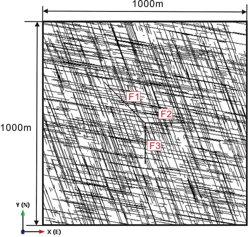
The lengths of the faults were 282.8, 200, and 200 m. The three faults intersected at the centre of the model. The total number of fractures in the two different fracture sets is 1600. The mean pole trends of these two sets of fractures were 10° and 70°, according to previous research (Wang et al. 2016). The mean equivalent radii of the two sets of fractures were set at 50 m. The permeabilities (k) of the two sets of stochastic fractures were set at 5 × 10³ mD (5 × 10⁻¹² m²), and the specific storage Ss was 1 × 10⁻⁶ m⁻¹. For the larger faults, the permeability was 1 × 10⁷ mD, and the specific storage was 1 × 10⁻⁶ m⁻¹. A transient flow model was used to obtain as much data as possible. In this simulated case, the six sides of the model were assigned no-flux boundaries.

2.3.2 Pumping experiment design

Nine boreholes were arranged, named W0–W8. The well locations are shown in Fig. 2(a). Detailed information about the pumping experiments (e.g. the pumping location coordinates and the relative positions of the pumping wells and large faults) is listed in Table 1. It should be noted that W0, W3, W5, and W8 were crossed by the nearest large faults, wherein W0 was crossed by F1, F2, and F3. To obtain more data from the limited wells, each well in the model was selected in turn to be a pumping well. When each pumping test was carried out, the remaining wells were treated as observation segments. The initial hydraulic head distribution was spatially uniform with a value of 100 m. The pumping operations lasted 5 d with a constant rate of 0.159 m³/d.

Table 1. Information about the pumping wells and the relative positions of the fault and pumping wells

Well no.	Pumping point oordinates: x	Pumping point coordinates: y	Relative position
0	500.000	502.609	Connected with F1, F2, and F3
1	500.000	700.859	–
2	700.000	704.540	–
3	700.000	501.150	Connected with F3
4	700.000	292.503	–
5	500.000	277.781	Connected with F2
6	279.747	300.000	–
7	300.000	502.467	–
8	296.333	700.000	Connected with F1

Figure 2. (a) Diagram of the well layout used to carry out hydraulic tomography analysis. The blue circles represent the nine pumping locations. (b) Diagram of the well layout used for validation. The blue circles represent the wells, and the pink circles (W02 and W04) represent the two pumping locations used in the validation analysis

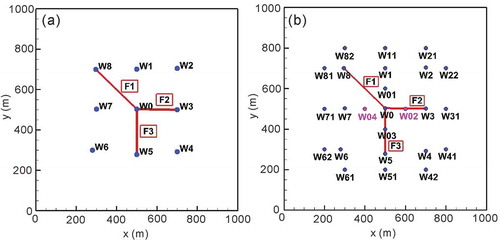
Furthermore, two independent pumping tests were carried out to validate the inversion results. To prove the inversion results for the entire area, the wells used for verification were refined and extended based on the layout used for the HT analysis. We set 12 wells on the outside and four wells on the inside of the original layout. There were 25 wells utilized for verification, as shown in Fig. 2(b). Meanwhile, W02 (between W0 and W3) and W04 (between W0 and W7) were set as pumping wells to carry out two pumping tests. In particular, W02 was connected to F2. During each pumping test, the remaining 24 wells were regarded as observation wells. The time of each pumping test was 5 d, and six groups of drawdown data were collected, at 0.1, 1, 2, 3, 4, and 5 d. The six boundaries of the verification model were set as no-flux boundaries. Two pumping tests were conducted, then drawdown data were compared with the data from the forward simulation of the inversion parameter fields. Moreover, a particle tracking simulation was conducted to determine the connectivity of the fracture system in this study (see Supplementary material, Fig. S1).

2.4 Inversion case design

The head values at eight observation wells in nine pumping tests were used for inversion in the VSAFT2 (Variably Saturated Flow and Transport in 2-Dimensions) software. Three sets of head values were chosen based on the different time periods from the transient head values calculated in the forward simulation. The result was validated with the particle tracking simulation and the transient data from two independent pumping tests.

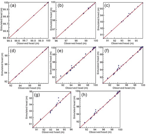
Case 1 was implemented to study the feasibility of the inversion results based on the static data. In this case, the effect of different observed data at various times was investigated. To examine the differences between the results of the static and transient data, the hydraulic properties were estimated using the transient data. This case was identified as Case 2. In this case, the strategy of choosing separate observation wells was investigated. In addition, the differences between the results when Ss was and was not estimated were investigated. Finally, the effect of the grid size in the inversion models was examined in Case 3. In Case 1 and Case 2, the grid size in the inversion models was set to 20 m × 20 m, and there were 2500 cells (2601 nodes) in these models (Fig. 3(a)). The grids of the models in Case 3 were refined, and the number of grids and nodes increased to 5329 and 5476, respectively, which is shown in Fig. 3(b). The initial guesses for K, Ss, and the correlation scales in the three cases are shown in Table 2. There were eight scenarios in total, among the three cases. The calibration results of the eight simulations are presented in Fig. 4. The calibration results indicate that all the observed head data were in good agreement with the simulated head data in the pumping tests used for inversion.

Table 2. Initial guesses for K and Ss, and correlation scales of the three cases

	K (m/d)	Ss (m^−1)	Correlation scale (m)
Case 1a	10	1.00 × 10^−7	200
Case 1b	10	1.00 × 10^−7	200
Case 1c	10	1.00 × 10^−7	200
Case 2a	0.1	1.00 × 10^−6	100
Case 2b	0.1	1.00 × 10^−6	100
Case 2c	0.1	1.00 × 10^−6	100
Case 3a	10	1.00 × 10^−7	200
Case 3b	0.1	1.00 × 10^−6	100

Figure 3. (a) Grid patterns used in Cases 1 and 2. (b) Grid pattern used in Case 3, which was refined based on the grid in Case 1. The green circles denote the pumping locations

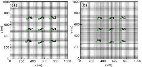
Figure 4. Head scatter plots of the calibration results in the three cases. Calibration results of (a–c) Case 1a–c, (d–f) Case 2a–c, and (g–h) Case 3a–b. The red dashed line in each graph shows a linear fit of the data, and the black line denotes the 1:1 line indicating a perfect match

3 Results and discussion

3.1 Applicability of static data at different times for parameter estimation

The static data were used in Case 1, namely the head values of nine pumping tests at 0.1, 1, and 5 d. Contour maps of the K field at the three time points are shown in Fig. 5(a–c). K and Ss were estimated simultaneously in this case. The initial guess for K was 10 m/d, and the initial guess for Ss was 1 × 10⁻⁷ m⁻¹. Since the DFN model ignores the matrix effects and the model was shown to be an equivalent continuum model after using the SLE algorithm, the inversion results of K contained high variance. From Fig. 5(a), a vague pattern was obtained using the steady-state data at 0.1 d. This is reasonable partly because the head contour affected a relatively small area after short times. Figure 5(c) shows the estimated K field using the static data at 5 d. As expected, the locations of three large faults were evident. Meanwhile, when the aggregate time was used in the static inversion, the variance of K gradually decreased. The fractures between W2 and W3 exhibited relatively better connectivity than the other areas, which will be verified below.

Figure 5. Contour maps of estimated K fields and validation results in Case 1 with the static data. Estimated K fields and validation results using the data at (a, d) 0.1 d, (b, e) 1 d, and (c, f) 5 d are presented. In (a–c), the black circles represent the nine pumping locations, and the black lines represent the large fractures. In (d–f), the red dashed line shows a linear fit of the data, and the black line is the 1:1 line indicating a perfect match

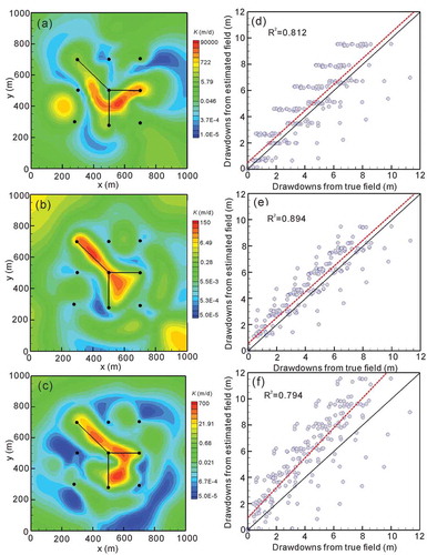
A linear model was utilized to fit the scatter data. All statistics of the verification criteria in the three cases are presented in Table 3. Figure 5(d–f) clearly shows the accuracy of the model in each case using static data. The longer term head data were further found to increase the R² and decrease L1 and L2 in Cases 1a and 1b. The high-K zones in Case 1c were more vivid than those in Case 1b. However, the verification results of these two cases were very similar. This is because the data of the static case at 1 d may have been sufficient to show the effect on all the observed wells. It is equally important to choose an appropriate time when using steady-state data for inversion. Overall, the quantitative verification results were in agreement with the K field and the actual data, which indirectly proved our hypothesis that a set of longer term data produced better results.

Table 3. Statistics of the validation criteria for the estimated hydraulic conductivity fields in Cases 1–3

		R^2	L1 (m)	L2 (m^2)	Slope	Intercept (m)
Case 1	a	0.812	1.032	2.001	0.993	0.516
	b	0.894	0.845	1.197	0.983	0.617
	c	0.794	1.771	4.890	1.143	0.919
Case 2	a	0.824	0.839	1.448	0.917	0.282
	b	0.299	2.165	10.734	0.482	−0.172
	c	0.858	0.732	1.130	0.880	0.294
Case 3	a	0.829	1.234	2.660	1.077	0.587
	b	0.860	0.721	1.097	0.887	0.329

3.2 Applicability of transient data for parameter estimation

The transient data were utilized to estimate the K field to test whether better results could be obtained in Case 2. Three scenarios were examined in this case, and the inversion results are shown in Fig. 6. The initial guesses for K and Ss in the scenarios were 0.1 m/d and 1 × 10⁻⁶ m⁻¹, respectively. The head data of four pumping tests were used in the first scenario (Fig. 6(a)), and the results showed a relatively inaccurate zone for the three big faults, especially the location of F1. Compared with Fig. 6(c), the estimated high-K zones with the data from nine pumping tests were more consistent with the actual locations of large faults. This led to the conclusion that more data fusion could create a more accurate estimated K pattern, a conclusion also reached by Zha et al. (2014) and Hao et al. (2008).

Figure 6. Contour maps of estimated K fields and validation results in Case 2 with the transient data. (a, d) Estimated K field and validation results using the data from four pumping tests at W0, W3, W5, and W8 (pink rectangles), where K and Ss were estimated simultaneously. (b, e) Estimated K field and validation results using the data from nine pumping tests without estimating Ss. (c, f) Estimated K field and validation results using the data from nine pumping tests, where K and Ss were estimated simultaneously. In (a–c), the black circles represent the nine well locations, and the black lines represent the large fractures. In (d–f), the red dashed line represents a linear fit of the data, and the black line is the 1:1 line indicating a perfect match

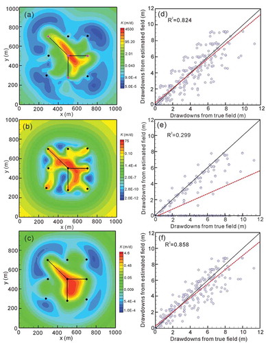
The effect of estimating Ss was further studied. The range of perturbations of lnK in Case 2b was from −24.5 to 6.6, which was significantly larger than the perturbation of the K value in Case 2c. Ss was set at the same value in the inversion model of Case 2b. The grids with uniform Ss values tried to adjust the head differences by modifying the K value. Thus, an estimated K field with high variance was obtained. There was a significant improvement in the pattern of the high-K zones in Case 2c compared with the previous two scenarios. In particular, the location of F1 was more accurately described, and the other faults were described well overall.

The verification of the inversion using transient data is presented in Fig. 6(d–f). The verification results of the inversions based on transient data were significantly better than those based on static data. The R² values of the verification results in Cases 2a and 2c were 0.824 and 0.858, respectively. The main reason was speculated to be that the four pumping locations in Case 2a were all set on large faults, and the distribution of surrounding fractures was almost uniform. With a proper arrangement of the pumping locations, less data in a DFN model could be used to obtain reasonable inversion results. As excepted, verification results in Case 2b were inaccurate because a constant Ss was given in each grid during the HT analysis. Thus, for the transient HT analysis using the data from a DFN model, K and Ss should be estimated simultaneously.

3.3 Applicability of refined grids for parameter estimation

The grids were refined to obtain a more detailed result in Case 3. The inversion results of Case 3 are shown in Fig. 7(a–b). The static data at 5 d (Case 3a) and the transient data (Case 3b) were utilized in this case. The high-K zones in Case 3 were narrow compared with the patterns in Cases 1c and 2c. There was a good consistency between the high-K zones and the positions of three faults.

Figure 7. Contour maps of estimated K fields and validation results in Case 3 using the refined grid. (a, c) Estimated K field and validation results using the data at 5 d of nine pumping tests and (b, d) the transient data of nine pumping tests are presented. In (a, b), the black circles represent the nine pumping locations, and the black lines represent the large fractures. In (c, d), the red dashed line represents a linear fit of the data, and the black line is the 1:1 line indicating a perfect match

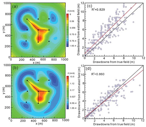
The verification results of the refined model in Case 3 are presented in Fig. 7(c–d). The R² increased to 0.860 compared with that in Case 2c, and L1 and L2 decreased to 0.721 and 1.097, respectively. L1 and L2 in Case 3a also decreased – to 1.234 and 2.660, respectively – compared with Case 1c. The verification results showed the model with the refined grids produced a better inversion result.

4 Discussion

The statistics of the verification criteria for the estimated hydraulic conductivity fields in the three cases are presented in Table 3. The verification results for Case 1b were better than those for Case 1a. This is reasonable because the groundwater flowed farther, over a longer time. The estimated parameter field was more accurate when more pumping tests were used, in Case 2. The best R² in Case 2 was 0.858. Moreover, for the transient HT analysis, K and Ss should be estimated simultaneously, and the synchronous inversion of parameters has a great influence on the results. It was also found that the refined grids produced better results than the primary grids. However, the use of excessive data in inversion calculations may cause waste of time and money.

It is notable that the deviation in the value of hydraulic conductivity between Figs 5(c) and 6(c) is due to the different data selection strategies. Formally, this large-magnitude deviation reflects the importance of data selection. In addition to using L1, L2, and other indicators to measure the reliability of the inversion results, the distribution and value of the hydraulic conductivity were also used to perform reliability analysis. Since the fracture is equivalent to a continuum with an extremely high hydraulic conductivity, when the fracture is considered in terms of its interaction with the surrounding matrix, the magnitude of the comprehensive hydraulic conductivity is unknown. In addition, the verification results of Cases 1b and 2c were better, and the hydraulic conductivity fields inverted by the two cases were mainly in the range of 10⁻⁵–10² m/d, which was consistent to a certain extent. Besides, the verification results show that Case 2c produced the best results. In situations where there is sufficient data, the final inversion result will be determined based on Case 2c or Case 3b. Therefore, the SLE inversion results based on different data are quite different, which also reflects the importance of the data selection strategy.

This study was conducted based on numerical experiments, and it is the first step for a series of follow-up field experiments. The relevant strategies formulated in this study will play a decisive role in actual field applications in the future.

5 Conclusion

This study focused on investigating the feasibility of HT in identifying the hydraulic properties in DFN models and in finding reasonable data selection strategies. Two hypotheses were verified. First, the feasibility of using HT to identify the hydraulic properties in DFN models with high heterogeneity was investigated successfully. Second, since the effects of storage are minimal, the flow behaves as quasi-steady flow, and the inverse model can use steady-state conditions to estimate K. For instance, the estimated K fields were consistent with the connectivity of the fracture network, and the verification criteria also proved the inversion results. Furthermore, some strategies for data selection for inversion were also acquired. Using the static head data to invert the DFN model was appropriate, and it was validated by Cases 1b and 1c. With the increase in the effect range of the pumping test, the steady-state data over a longer time yielded better results. In the fractured medium with high heterogeneity, K and Ss should be estimated simultaneously. In addition, four pumping tests conducted on the large faults were sufficient to give a reasonable result in our DFN model. The results using data from nine pumping tests produced the best results, although this was time-consuming and costly.

As described by Hao et al. (2008), the K variations in fractured rock can exceed those used in their study (factor of 100) by several orders of magnitude in field situations. The inversion becomes highly nonlinear and difficult to simulate. This is the reason that the verification results were not as good as those obtained by Zha et al. (2014), where an EPM model was used to conduct inversion simulations. Finally, the results of this study proved the feasibility of HT to identify the hydraulic properties in a highly heterogeneous medium. This study advances the HT characterization of fractured media. The robustness of HT has been further verified, and more data fusion can produce better results for fracture network identification.

Acknowledgements

We thank the University of Arizona and the Institute of Geology and Geophysics of the Chinese Academy of Sciences. We are also very grateful to the anonymous reviewers for their constructive comments on this article.

Disclosure statement

No potential conflict of interest was reported by the authors.

Supplementary material

Supplemental data for this article can be accessed here.

Additional information

Funding

This work was supported by the National Key R&D Program of China [grant number 2018YFC1800204].

References

- Araujo, H., et al., 2004. Dynamic behavior of discrete fracture network (DFN) models. SPE international petroleum conference in Mexico, society of petroleum engineers. Mexico, Puebla Pue.
- Basquet, R., Bourbiaux, B.J., and Cohen, C.E., 2005. Fracture flow property identification: an optimized implementation of discrete fracture network models. SPE Middle East oil and gas show and conference, society of petroleum engineers. Bahrain, Manama.
- Basquet, R., et al., 2004. Gas-flow simulation in discrete fracture-network models. SPE Reservoir Evaluation & Engineering, 7 (5), 378–384. doi:https://doi.org/10.2118/88985-PA
- Benke, R. and Painter, S., 2003. Modeling conservative tracer transport in fracture networks with a hybrid approach based on the Boltzmann transport equation. Water Resources Research, 39 (11), 1–11. doi:https://doi.org/10.1029/2003WR001966
- Blessent, D., Therrien, R., and Gable, C.W., 2011. Large-scale numerical simulation of groundwater flow and solute transport in discretely-fractured crystalline bedrock. Advances in Water Resources, 34 (12), 1539–1552. doi:https://doi.org/10.1016/j.advwatres.2011.09.008
- Bodin, J., et al., 2007. Simulation and analysis of solute transport in 2D fracture/pipe networks: the SOLFRAC program. Journal of Contaminant Hydrology, 89 (1–2), 1–28. doi:https://doi.org/10.1016/j.jconhyd.2006.07.005
- Browning, L., et al., 2003. Reactive transport model for the ambient unsaturated hydrogeochemical system at Yucca Mountain, Nevada. Computers & Geosciences, 29 (3), 247–263. doi:https://doi.org/10.1016/S0098-3004(03)00003-7
- Cheong, J.-Y., et al., 2017. Hydraulic parameter generation technique using a discrete fracture network with bedrock heterogeneity in Korea. Water, 9 (12), 937. doi:https://doi.org/10.3390/w9120937
- Dershowitz, W., et al., 1993. FracMan user documentation. Seattle: Golder Associates Inc.
- Dong, Y., et al., 2019. Equivalence of discrete fracture network and porous media models by hydraulic tomography. Water Resources Research, 55 (4), 3234–3247. doi:https://doi.org/10.1029/2018WR024290
- El Alfy, M., 2014. Numerical groundwater modelling as an effective tool for management of water resources in arid areas. Hydrolological Sciences Journal, 59 (6), 1259–1274. doi:https://doi.org/10.1080/02626667.2013.836278
- Hao, Y., et al., 2012. Differences in karst processes between northern and southern China. Carbonates and Evaporites, 27 (3–4), 331–342. doi:https://doi.org/10.1007/s13146-012-0116-3
- Hao, Y., et al., 2008. Hydraulic tomography for detecting fracture zone connectivity. Ground Water, 46 (2), 183–192. doi:https://doi.org/10.1111/j.1745-6584.2007.00388.x
- Hastings, W.K., 1970. Monte Carlo sampling methods using Markov chains and their applications. Biometrika, 57 (1), 97–109. doi:https://doi.org/10.1093/biomet/57.1.97
- Huang, S.-Y., et al., 2011. Robustness of joint interpretation of sequential pumping tests: numerical and field experiments. Water Resources Research, 47 (10), 1–18. doi:https://doi.org/10.1029/2011WR010698
- Illman, W.A., 2014. Hydraulic tomography offers improved imaging of heterogeneity in fractured rocks. Ground Water, 52 (5), 659–684. doi:https://doi.org/10.1111/gwat.12119
- Illman, W.A., Berg, S.J., and Yeh, T.C., 2012. Comparison of approaches for predicting solute transport: sandbox experiments. Ground Water, 50 (3), 421–431. doi:https://doi.org/10.1111/j.1745-6584.2011.00859.x
- Kelkar, S., et al., 2013. Breakthrough of contaminant plumes in saturated volcanic rock: implications from the Yucca Mountain site. Geofluids, 13 (3), 273–282. doi:https://doi.org/10.1111/gfl.12035
- Klepikova, M., Brixel, B., and Jalali, M., 2020. Transient hydraulic tomography approach to characterize main flowpaths and their connectivity in fractured media. Advances in Water Resources, 136, 103500. doi:https://doi.org/10.1016/j.advwatres.2019.103500
- Kuhlman, K.L., et al., 2008. Basin-scale transmissivity and storativity estimation using hydraulic tomography. Ground Water, 46 (5), 706–715. doi:https://doi.org/10.1111/j.1745-6584.2008.00455.x
- Liu, S., Yeh, T.C.J., and Gardiner, R., 2002. Effectiveness of hydraulic tomography: sandbox experiments. Water Resources Research, 38 (4), 5-1–5-9. doi:https://doi.org/10.1029/2001WR000338
- Liu, X., et al., 2007. Laboratory sandbox validation of transient hydraulic tomography. Water Resources Research, 43 (5), 1–13. doi:https://doi.org/10.1029/2006WR005144
- Liu, Y., et al., 2014. A nonstationary extreme value distribution for analysing the cessation of karst spring discharge. Hydrological Processes, 28 (20), 5251–5258. doi:https://doi.org/10.1002/hyp.10013
- Long, J., et al., 1982. Porous media equivalents for networks of discontinuous fractures. Water Resources Research, 18 (3), 645–658. doi:https://doi.org/10.1029/WR018i003p00645
- Lu, -C.-C., et al., 2005. Integration of transfer function model and back propagation neural network for forecasting storm sewer flow in Taipei metropolis. Stochastic Environmental Research and Risk Assessment, 20 (1–2), 6–22. doi:https://doi.org/10.1007/s00477-005-0243-7
- Mao, D., et al., 2013. Joint interpretation of sequential pumping tests in unconfined aquifers. Water Resources Research, 49 (4), 1782–1796. doi:https://doi.org/10.1002/wrcr.20129
- Michael Tso, C.-H., et al., 2016. The relative importance of head, flux, and prior information in hydraulic tomography analysis. Water Resources Research, 52 (1), 3–20. doi:https://doi.org/10.1002/2015WR017191
- Moench, A.F., 1984. Double‐porosity models for a fissured groundwater reservoir with fracture skin. Water Resources Research, 20 (7), 831–846. doi:https://doi.org/10.1029/WR020i007p00831
- Moreno, L., Crawford, J., and Neretnieks, I., 2006. Modelling radionuclide transport for time varying flow in a channel network. Journal of Contaminant Hydrology, 86 (3–4), 215–238. doi:https://doi.org/10.1016/j.jconhyd.2006.03.004
- Motakabbir, K.A. and Berkowitz, M., 1990. Isothermal compressibility of SPC/E water. Journal of Physical Chemistry, 94 (21), 8359–8362. doi:https://doi.org/10.1021/j100384a067
- Reeves, D.M., Benson, D.A., and Meerschaert, M.M., 2008. Transport of conservative solutes in simulated fracture networks: 1. Synthetic data generation. Water Resources Research, 44 (5), 1–10. doi:https://doi.org/10.1029/2007WR006069
- Robinson, P.C., 1984. Connectivity, flow and transport in network models of fractured media. Oxford, Oxfordshire, England: University of Oxford.
- Schwartz, M.O., 2012. Modelling radionuclide transport in large fractured-media systems: the example of Forsmark, Sweden. Hydrogeology Journal, 20 (4), 673–687. doi:https://doi.org/10.1007/s10040-012-0837-3
- Selroos, J.-O. and Painter, S.L., 2012. Effect of transport-pathway simplifications on projected releases of radionuclides from a nuclear waste repository (Sweden). Hydrogeology Journal, 20 (8), 1467–1481. doi:https://doi.org/10.1007/s10040-012-0888-5
- Spycher, N.F., Sonnenthal, E.L., and Apps, J.A., 2003. Fluid flow and reactive transport around potential nuclear waste emplacement tunnels at Yucca Mountain, Nevada. Journal of Contaminant Hydrology, 62, 653–673. doi:https://doi.org/10.1016/S0169-7722(02)00183-3
- Streltsova, T., 1976. Hydrodynamics of groundwater flow in a fractured formation. Water Resources Research, 12 (3), 405–414. doi:https://doi.org/10.1029/WR012i003p00405
- Sun, R., et al., 2013. A temporal sampling strategy for hydraulic tomography analysis. Water Resources Research, 49, 3881–3896. doi:https://doi.org/10.1002/wrcr.20337
- Wang, X., et al., 2016. Characterisation of the transmissivity field of a fractured and karstic aquifer, Southern France. Advances in Water Resources, 87, 106–121. doi:https://doi.org/10.1016/j.advwatres.2015.10.014
- Wen, J.-C., et al., 2010. Estimativa das propriedades hidráulicas efectivas de um aquífero em resultado de testes utilizando múltiplos furos de observação em Taiwan. Hydrogeology Journal, 18 (5), 1143–1155. doi:https://doi.org/10.1007/s10040-010-0577-1
- Williams-Stroud, S.C. and Eisner, L., 2010. Stimulated fractured reservoir DFN models calibrated with microseismic source mechanisms. 44th US rock mechanics symposium and 5th US-Canada rock mechanics symposium, American rock mechanics association. Salt Lake City, Utah, USA.
- Yan, B., et al., 2018. Multi-porosity multi-physics compositional simulation for gas storage and transport in highly heterogeneous shales. Journal of Petroleum Science and Engineering, 160, 498–509. doi:https://doi.org/10.1016/j.petrol.2017.10.081
- Ye, M., Khaleel, R., and Yeh, T.-C.J., 2005. Stochastic analysis of moisture plume dynamics of a field injection experiment. Water Resources Research, 41 (3), 1–13. doi:https://doi.org/10.1029/2004WR003735
- Yeh, T.-C., Khaleel, R., and Carroll, K.C., 2015a. Flow through heterogeneous geologic media. Cambridge (HQ), United Kingdom: Cambridge University Press.
- Yeh, T.C.J. and Liu, S., 2000. Hydraulic tomography: development of a new aquifer test method. Water Resources Research, 36 (8), 2095–2105. doi:https://doi.org/10.1029/2000WR900114
- Yeh, T.-C.J., et al., 2015b. Uniqueness, scale, and resolution issues in groundwater model parameter identification. Water Science and Engineering, 8 (3), 175–194. doi:https://doi.org/10.1016/j.wse.2015.08.002
- Yeh, T.-C.J., et al., 2009. River stage tomography: a new approach for characterizing groundwater basins. Water Resources Research, 45 (5), 1–14. doi:https://doi.org/10.1029/2008WR007233
- Yeh, T.‐.C.J. and Zhu, J., 2007. Hydraulic/partitioning tracer tomography for characterization of dense nonaqueous phase liquid source zones. Water Resources Research, 43 (6), 1–16. doi:https://doi.org/10.1029/2006WR004877
- Zha, Y., et al., 2015. What does hydraulic tomography tell us about fractured geological media? A field study and synthetic experiments. Journal of Hydrology, 531, 17–30. doi:https://doi.org/10.1016/j.jhydrol.2015.06.013
- Zha, Y., et al., 2014. Usefulness of flux measurements during hydraulic tomographic survey for mapping hydraulic conductivity distribution in a fractured medium. Advances in Water Resources, 71, 162–176. doi:https://doi.org/10.1016/j.advwatres.2014.06.008
- Zha, Y., et al., 2016. An application of hydraulic tomography to a large-scale fractured granite site, Mizunami, Japan. Ground Water.
- Zhang, Z., Li, X., and He, J., 2016. Numerical study on the permeability of the hydraulic-stimulated fracture network in naturally-fractured shale gas reservoirs. Water, 8 (9), 393. doi:https://doi.org/10.3390/w8090393
- Zhu, J. and Yeh, T.-C.J., 2005. Characterization of aquifer heterogeneity using transient hydraulic tomography. Water Resources Research, 41 (7), 1–10. doi:https://doi.org/10.1029/2004WR003790
- Zhu, J. and Yeh, T.-C.J., 2006. Analysis of hydraulic tomography using temporal moments of drawdown recovery data. Water Resources Research, 42 (2), 1–11. doi:https://doi.org/10.1029/2005WR004309