Non-stationary flood frequency analysis and attribution of streamflow series: a case study of Periyar River, India

ABSTRACT

The occurrence of extreme hydrological flood events has become frequent recently, especially in India. Flood analysis methods need to capture variations in trends and identify key factors causing this variation. Non-stationary flood frequency analysis is one of the few methods that can account for these variations. In this study, the non-stationarity of Periyar River discharge was investigated through the flood frequency analysis of one stationary and 12 non-stationary models, produced using a generalized extreme value distribution with annual precipitation, urban extent and time as a linear function of its location and scale parameter. The analysis found that both climate change and anthropogenic activities are responsible for the non-stationarity of the Periyar River discharge. Also, the 50-year return level of the stationary model was found to be equal to the 39-year return level of the optimal non-stationary model, thus, the assumption of stationarity may lead to the unsafe design of structures.

KEYWORDS:

• non-stationarity
• flood frequency analysis
• return period
• climate change
• urbanization
• Indian floods

Editor A. Castellarin Associate Editor I. Prosdocimi

1 Introduction

Floods are caused when rivers cannot contain the upstream runoff within their banks. Floods are intensified by natural phenomena such as a reduction in the carrying capacity of the river due to erosion and silting of the river bed, landslides and earthquakes causing obstruction and change in river paths, or simultaneous floods in main and tributary rivers; and by anthropogenic phenomena such as encroachment of floodplains and unplanned urban settlements (Salas and Obeysekera 2014; Chinnasamy and Sood 2020, Chinnasamy et al. 2020). In India, more than 40 million hectares of land, or 12% of the geographical area, is flood-prone, and every year over 1600 people die due to floods, with damages costing over Rs. 5600 crores (73 million USD) annually (Central Water Commission 2018).

To protect against floods in India, structural measures like flood defences, dams, and reservoirs have been adopted (Chinnasamy et al. 2021). For designing these hydraulic structures and to better understand the occurrence of floods based on the concepts of the return period, risk and reliability, a wide range of statistical techniques have been developed, such as probability distribution functions, time series models, stochastic models, and physically based watershed models (Salas et al. 2018). These techniques and models have generally been developed with the assumption that hydrological events have stationarity (Merz et al. 2012). Stationarity is the property of a system according to which the statistical parameters like the mean and variance of the system do not change with time and exhibit no trend (Sivakumar 2016). However, under the influence of climate change, land use/land cover change, and construction of river regulation structures, the assumption of stationarity may no longer be valid (Ray and Goel 2019). Thus, alternative methods that incorporate the consideration of non-stationarity need to be developed, for the effective design, planning, and management of hydraulic structures (Salas et al. 2018).

Statistical methods are used globally for the detection of non-stationarity in streamflow time series (Salas and Obeysekera 2014). As per Machiwal and Jha (2009), non-stationarity of a time series statistically indicates the presence of a trend, because of which two sample series of the population time series may look similar but would be scattered around different mean values. These sample series with different mean values signify the presence of a change in the distribution of the population time series, and the locations at which they are separated are called change points (Ryberg et al. 2020). Trend tests like Mann-Kendall test (Jaiswal et al. 2015), along with change point tests like the pruned exact linear time method (Haynes et al. 2017), the E-divisive method (Matteson and James 2014), the change point procedure via pruned objectives (Zhang et al. 2017), and the Pettitt test (Faulkner et al. 2020), have been used widely to detect the presence of non-stationarity in streamflow time series.

For optimum flood frequency analysis, both detection and attribution of non-stationarity are important. The process of finding the variables responsible for the non-stationarity of hydrological events is called attribution (Merz et al. 2012). These variables are termed covariates, and can be associated with a natural or an anthropogenic phenomenon. Serago and Vogel (2018) and Kang et al. (2020) used time as the covariate, considering it a proxy for all changing physical phenomena. But this implies that the non-stationarity in the streamflow time series will remain indefinitely. Thus, for the attribution of non-stationarity, it is crucial to analyse the influence of physical covariates.

The physical covariates that can be used to accommodate the non-stationarity of streamflow time series due to natural phenomena include annual precipitation (Faulkner et al. 2020) and downscaled meteorological variables from general circulation models (GCMs) (Du et al. 2015). At present, GCMs work only on a coarse spatial and temporal scale, and thus need robust downscaling to basin scale (Salas and Obeysekera 2014). Also, the uncertainty associated with these models may lead to inaccurate flood frequency analysis and risk estimation (Faulkner et al. 2020). On the other hand, the annual precipitation that encompasses the effects of climate change relates closely to the catchment soil moisture and other catchment characteristics, and thus can be used for the attribution of non-stationarity. The covariates that can represent anthropogenic phenomena are the urban extent (Prosdocimi et al. 2015), population (Yan et al. 2017), and reservoir index (Ray and Goel 2019). These covariates can be used according to the prevailing conditions of the study site.

The detection and attribution of non-stationarity of streamflow time series have been carried out using sophisticated models such as vector generalized additive models (VGAMs) (Yee and Wild 1996), vector generalized linear models (VGLMs) (Yee and Stephenson 2007) and generalized additive models in location, scale, and shape (GAMLSS) (Rigby and Stasinopoulos 2005), but to implement these models it is important to thoroughly understand these advanced tools to avoid incorrect conclusions (Serinaldi and Kilsby 2015). In contrast, regression analysis can be more convenient for characterizing the non-stationarity of streamflow time series (Salas et al. 2018). In regression analysis a single equation can be used to estimate all conditional moments required for non-stationary flood frequency analysis, and multivariate regression can incorporate multiple covariates to represent multiple influencing phenomena (Condon et al. 2015, Prosdocimi et al. 2015).

In India, due to the rising frequency and volume of extreme events (Central Water Commission 2018), it is crucial to incorporate non-stationary flood frequency analysis for water resources planning and management. The application of this approach is demonstrated using a case study of the Periyar River basin. Over the past few decades, the Periyar River basin of the southern state of Kerela in India has experienced an increase in extreme flood events (Madhusoodanan 2018). In 1924, due to heavy rain and high wind speed, the Periyar River experienced the worst flood of the decade, with the average rainfall being 64% (3368 mm) higher than the normal rainfall (Hunt and Menon 2020). In 1961, a long duration of high-intensity rainfall flooded the Periyar River basin, due to which 115 people lost their lives (CWC 2018). In 2018, Kerala experienced rainfall 53% higher than normal, resulting in a loss of more than 400 lives (Amritanand et al. 2020) and an economic loss of more than Rs. 200 billion, primarily in the Periyar River basin (Lal et al. 2020). However, flood frequency analysis of the Periyar River including a consideration of factors influencing the variations in streamflow has not been conducted, even though such study is vital for safe design, planning, and water resources management.

The specific objectives of this study are to: (1) identify the presence of non-stationarity in Periyar River streamflow series; (2) detect change points in the streamflow series to find the location of non-stationarity; (3) fit stationary and non-stationary generalized extreme value (GEV) distributions to streamflow series with annual precipitation, urban extent, and time as covariates; and (4) obtain the optimum GEV distribution for efficient flood frequency analysis.

2 Study area

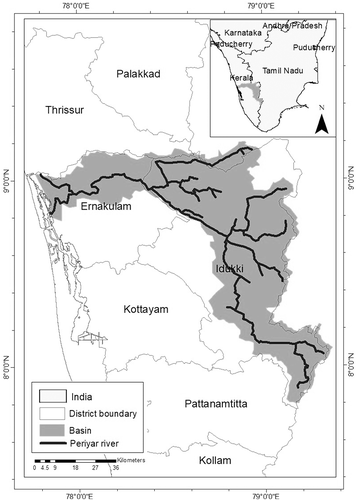
Kerala, the most southwestern state of India, lies between latitudes 8°17’30” and 12°47’40”N and longitudes 74°27’47” and 77°37’12” E. The longest river of Kerala is the Periyar River, which is considered as its lifeline. The total length of the Periyar River is 300 km and the total drainage area of Periyar inside Kerala is 5284 km², as shown in Fig. 1. The river originates at the Sivagiri peaks of Sundaramala in Tamil Nadu. The major tributaries of the Periyar are Mullayar, Perumthurai Aar, Kattapanayar, Cherutohnniyar, Chittar, Perinjankutty Aar, Muthirapuzha, Thottiyar and Idamalayar. At Alwaye, the river bifurcates into two streams, Mangalapuzha and the Marthanadavarma, and then, after forming various islands, joins the Arabian Sea (Priju et al. 2018).

Figure 1. Periyar River and basin in Tamil Nadu and Kerala states of India

In the Periyar River basin, 28% of the area is covered by forest; however, due to various development activities such as hydroelectric projects, and human settlements, a large part of the forest cover has been removed (Sudheer et al. 2019).

3 Hydrological data and pre-processing

In this study, for the flood frequency analysis, daily streamflow data of the Neeleshwaram gauging site (maintained by the Central Water Commission) were used. The Neeleshwaram gauging site is situated at the downstream of Periyar River in the Ernakulam district of Kerala. For this study, 40 years’ daily streamflow data, from 1979 to 2018, were downloaded from the Water Resources Information System of India (India WRIS 2020).

For modelling the extreme hydrological variables, the concept of block maxima was used, which involves dividing the whole observation period into non-overlapping periods of equal size and focusing on the maximum value of each period (Gumbel 1958). The block maxima series for the Neeleshwaram site was obtained by dividing the observation period of 40 years from 1979 to 2018 chronologically into equal-sized non-overlapping periods of 365 d and considering the maximum observation of each period.

In this study, non-stationary streamflow block maxima were modelled with the covariates representing natural phenomena and human interference. In a basin, precipitation can depict the impacts of climate change and relates closely to the soil moisture along with the other basin characteristics; thus it can be used as a covariate to represent natural phenomena. The Periyar River basin experiences precipitation during the whole year; the precipitation seasons can be divided into pre-monsoon (March to May), southwest monsoon (June to September), post-monsoon (October to November), and winter (December to February). The contributions of these four seasons towards the annual precipitation of the basin are 13.10%, 67.85%, 6.46% and 2.58%, respectively, where the annual precipitation (AP) is defined as the sum of the daily rainfall for a particular year. In this study, the AP series was built using the daily precipitation data of the Periyar River basin for the period 1979–2018. The annual precipitation and seasonal precipitation can be considered covariates. Thus, the annual and seasonal precipitation were examined using the Spearman rank correlation test, to obtain the strength of their correlation with the streamflow block maxima. The Spearman rank correlation coefficient (rho) of AP with the streamflow block maxima (rho = 0.43) was found to be better than that of pre-monsoon precipitation (rho = 0.03), southwest monsoon (rho = 0.36), post-monsoon precipitation (rho = 0.26) and winter precipitation (rho = −0.03), which indicates that the seasonal precipitation had lower correlation compared to the annual precipitation, thus the seasonal precipitation will not be considered further in this study.

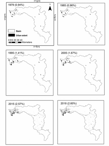
The change in land use in a basin indicates the influence of human interference. The urban extent that corresponds to the impervious area of the basin is responsible for the rise in peak, volume and reduction of the time of concentration of flood. Thus, for the Periyar River basin, the non-stationarity of streamflow block maxima was analysed with the percentage urban extent (URBEXT) as the covariate representing the human interference (Prosdocimi et al. 2015). To construct the URBEXT series, the urban extent in 1979, 1985, 1995, 2005, 2015, and 2018 was obtained by performing unsupervised classification (Henderson et al. 2009) of the Landsat, Resourcesat1 and Resourcesat2 land-use maps of the study area in Geographic Information System (GIS) software as shown in Fig. 2, and then the obtained percentage of urban extent was fitted to a polynomial function to generate the URBEXT time series.

Figure 2. Evolution of urban extent in the Periyar basin in Kerala. The year to which the image refers is indicated along with the urban extent percentage in parentheses

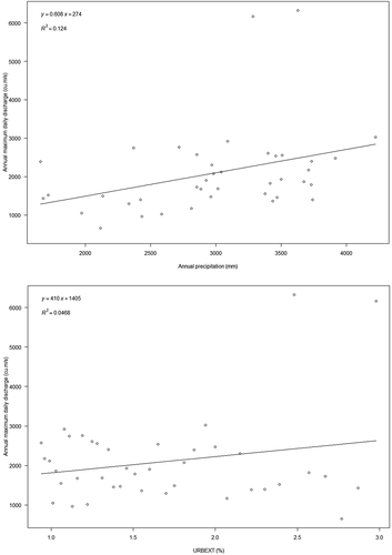
The linear trend of the covariates AP and URBEXT against streamflow block maxima are depicted in Fig. 3. The linear trend of streamflow block maxima against AP is rising at a rate of 0.61 m³ s⁻¹ mm⁻¹, with a linear correlation coefficient (r) of 0.35; and the linear trend of streamflow block maxima against URBEXT is rising at a rate of 410 m³ s⁻¹ urbext%⁻¹, with r = 0.21, as shown in Fig. 3. The trend lines indicate that the streamflow block maxima are rising with the rise in AP and URBEXT.

Figure 3. Scatter plot and linear correlation of the covariates AP and URBEXT with the streamflow block maxima

In many studies, time alone has been used as the covariate (Serago and Vogel 2018, Kang et al. 2020), considering it a proxy for all changing physical phenomena. Thus, to evaluate the suitability of this assumption, the non-stationary streamflow block maxima were modelled using time also. The series for covariate time was built using the year of streamflow block maxima (Um et al. 2017).

4 Statistical analysis

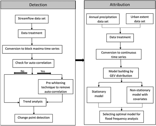
In this study, the non-stationary flood frequency analysis has been carried out in two stages. In the first stage, detection of non-stationarity was done using the non-parametric trend test and non-parametric change point detection. Before using the trend test, the auto-correlation test was conducted to detect temporal correlation of hydrological data, which may lead to false trend detection. In the second stage, attribution was done by fitting the block maxima to a GEV distribution using time, annual precipitation, and urban extent as a linear function of its location and scale parameter. These steps are shown in Fig. 4.

Figure 4. Flowchart depicting the methodology for non-stationary flood frequency analysis

4.1 Trend analysis

The non-parametric Mann-Kendall (MK) test is employed to detect monotonic trends in a series of hydrological data (Mann 1945). The MK test statistic for a time series is expressed by Equation (1)(1) $\mathrm{S}={\sum }_{k=1}^{n-1}{\sum }_{k+1}^n\mathrm{s}\mathrm{g}\mathrm{n}\left(x_j-x_k\right)$(1) :

(1) $\mathrm{S}={\sum }_{k=1}^{n-1}{\sum }_{k+1}^n\mathrm{s}\mathrm{g}\mathrm{n}\left(x_j-x_k\right)$(1)

where “sgn” is the signum function. The statistic “S” is considered approximately normally distributed, with mean µ = 0, and the variance is given by Equation (2):

(2) ${\sigma }^2=\frac{\left\{n\left(n-1\right)\left(2n+5\right)\right\}}{18}$(2)

Here, “x” is the variable and “n” denotes the number of data, and “i,” “j,” and “k” are indices.

In this study, the streamflow block maxima series was examined for trends using the MK test, with a 95% confidence interval, to evaluate the non-stationarity of the series (Pohlert 2020).

While using the MK trend test, it is vital to check the temporal correlation of the time series, as the presence of correlation in time series influences the process of trend detection (Gado 2016). The influence of auto-correlation can be removed by pre-whitening (Yue et al. 2003) or by using the modified MK test (Hamed and Rao 1998). Thus, MK test with pre-whitening, and its variations such as the modified MK test, can be used to observe the trend of a non-parametric and temporally correlated dataset.

4.2 Change point analysis

The change points in a hydrological event can be evidence of natural or anthropogenic changes and non-stationarity (Ryberg et al. 2020). To conduct a change point analysis, opting for a non-parametric test would be appropriate, as a parametric test is conducted with the assumption that the time series follows a normal distribution, while in reality streamflow time series tend to have a skewed distribution. Also, the test should be capable of finding multiple change points because in prolonged data series there can be multiple significant change points (Salas et al. 2018).

In the literature, multiple change point tests are mentioned and used, but their application for different purposes has not been defined clearly. Thus, in this study four non-parametric change point methods were applied and compared, which are the (i) nonparametric pruned exact linear time method (PELT; Haynes et al. 2017); (ii) E-divisive method (Matteson and James 2014); (iii) change point procedure via pruned objectives (CP3O; Zhang et al. 2017); and (iv) Pettitt test (Pettitt 1979).

Using multiple tests for change point detection can help to avoid false positives and subsequently lead to an appropriate change point test. Amongst these tests, the PELT method gives better computational efficiency (Haynes et al. 2017), the E-divisive test involves fewer assumptions (Matteson and James 2014), the CP3O has been determined to give better accuracy for a particular computation time (Zhang et al. 2017), and the Pettitt test is the most commonly used change point test but is restricted by the number of change points.

4.2.1 Nonparametric pruned exact linear time method

The PELT algorithm is an accurate method for change point detection, with O(n) as the computational efficiency (Wambui et al. 2015). It also gives better computational speed than other methods (Ryberg et al. 2020). In this study, the PELT algorithm was applied using the “changepoint.np” package of R. In this package, the PELT method was built as a modification of the optimal partitioning method, to improve the computational efficiency. The essence of pruning lies in the elimination of specific “τ” (location of a change point) values which can never be a minimum value of the minimization performed at each iteration (Haynes et al. 2017). The non-parametric PELT test is developed as an extension of the univariate change point detection carried out by a nonparametric likelihood empirical distribution (Zou et al. 2014).

The assumption of the PELT test is that there exists a constant K with the condition shown in Equation (3)(3) $C\left(x_{\left(\mathrm{t}+1\right):\mathrm{s}}\right)+C\left(x_{\left(\mathrm{s}+1\right):\mathrm{T}}\right)+\mathrm{K}\le C\left(x_{\left(\mathrm{t}+1\right):\mathrm{T}}\right)$(3) for all t < s < T

(3) $C\left(x_{\left(\mathrm{t}+1\right):\mathrm{s}}\right)+C\left(x_{\left(\mathrm{s}+1\right):\mathrm{T}}\right)+\mathrm{K}\le C\left(x_{\left(\mathrm{t}+1\right):\mathrm{T}}\right)$(3)

And, if Equation (4)(4) $F\left(t\right)+C\left(x_{\left(\mathrm{t}+1\right):\mathrm{s}}\right)+\mathrm{K}\ge F\left(s\right)$(4) holds,

(4) $F\left(t\right)+C\left(x_{\left(\mathrm{t}+1\right):\mathrm{s}}\right)+\mathrm{K}\ge F\left(s\right)$(4)

at a future time T > s, then “t” can never be the optimal last change point prior to “T” of the data. With “n” as the length of series, initialized as F (0) = −β, cp (0) = NULL and R1 = {0}, then iterate for τ* = 1 …, n, over the following steps, where “β” is the penalty constant which does not depend on the number or location of change points. “C” is the cost function of a segment of the data, the minimization of the cost placed on all the segments helps to find the change point and “K” can be obtained from Equation (5)(5) $\epsilon \left(X,Y;\alpha \right)=2E{\left|X-Y\right|}^{\alpha }-E{\left|X-X{ }^{\mathrm{\prime }}\right|}^{\alpha }-E{\left|Y-Y{ }^{\mathrm{\prime }}\right|}^{\alpha }$(5) . The steps involved are the following:

1. Calculate F(τ*) = min _τ∈Rτ* [F(τ) + C(x_{(τ+1): τ*}) + β].

2. Let τ¹ = arg {min _τ∈Rτ* [F(τ) + C(x_{(τ+1): τ*}) + β]}.

3. Set cp(τ*) = [cp(τ¹), τ¹].

4. Set R_τ*+1 = {τ ∈R _τ* ∪ {τ*}: F(τ) + C(x_{(τ+1): τ*}) +K < F (τ*)}.

Then, the output is the change points recorded in cp(n) (Killick and Eckley 2014).

The PELT algorithm of the “changepoint.np” package of R utilizes the above-described function to find multiple changes in the dataset (Haynes et al. 2016).

4.2.2 E-divisive

The E-divisive change point detection method is a non-parametric technique that combines the method of bisection with a multivariate divergence measure without making any assumptions beyond the existence of the $\alpha \mathrm{t}\mathrm{h}$ absolute moment (Matteson and James 2014). The divergence measure based on the Euclidian distance can be defined by Equation (5):

(5) $\epsilon \left(X,Y;\alpha \right)=2E{\left|X-Y\right|}^{\alpha }-E{\left|X-X{ }^{\mathrm{\prime }}\right|}^{\alpha }-E{\left|Y-Y{ }^{\mathrm{\prime }}\right|}^{\alpha }$(5)

where X and Y are two identically distributed vectors and X’ and Y’ are independent copies of X and Y.

For “n” independent observations of X and “m” independent observations of Y, the scaled empirical divergence can be obtained from Equation (6):

(6) $Q(X_{\mathrm{n}},Y_{\mathrm{n}};\alpha =\frac{mn}{m+n}\epsilon \left(X_{\mathrm{n}},Y_{\mathrm{m}};\alpha \right)$(6)

As per Matteson and James (2014), in the E-divisive method, several change points are detected by hierarchical statistical testing. Initially, the location of the change point is obtained by an iterative method. If (k − 1) change points are assumed to exist at 0 < τ1 < τ2 < τ3 < … … < τ (k − 1) < T, then these change points divide the dataset into “k” clusters C1, C2, C3 … … Ck. In these clusters single change points are found, considering Ci as the ith cluster with τ (i) as the location of the change point and κ(i) as the associated constant.

The test statistic to obtain the position of change point is given by Equation (7)(7) $q_k=Q\left(X_{{\tau }_{\mathrm{k}}},Y_{{\tau }_k}\left({\kappa }_k\right);\alpha \right)$(7) :

(7) $q_k=Q\left(X_{{\tau }_{\mathrm{k}}},Y_{{\tau }_k}\left({\kappa }_k\right);\alpha \right)$(7)

in which $X_{{\tau }_{\mathrm{k}}}$ and $Y_{{\tau }_{\mathrm{k}}}\left({\kappa }_{\mathrm{k}}\right)$ are defined concerning Ci.

After finding the location of change points, their significance is investigated. Large values of “${\mathrm{q}}_{\mathrm{k}}$” represent a significant change in the distribution of the clusters. To obtain the precise location of a change point, knowledge of the underlying distribution is required, which can be obtained by a permutation test. This whole process is repeated to obtain a significant change point. In this study, the E-divisive approach is applied using the ‘ecp’ library of the R program (James and Matteson 2015).

4.2.3 Change point procedure via pruned objectives

This method is a non-parametric change point detection approach, which uses a general procedure to find change points, based on a large number of goodness-of-fit metrics. Incorporation of some additional information like the type of changes to be observed or expected computational time may direct the researcher towards a particular goodness-of-fit metric. The CP3O procedure uses dynamic programming with pruning. Two types of change point algorithms of CP3O are E-CP3O and KS-CP3O, which incorporate E-statistics and Kolmogorov-Smirnov statistic goodness-of-fit metrics, respectively, in the CP3O search procedure (Zhang et al. 2017). In this study, the CP3O approach with E-statistics and Kolmogorov-Smirnov statistic as the goodness-of-fit measure is applied using the ‘ecp’ library of the R program (James and Matteson 2015).

4.2.4 Pettitt test

Pettitt test is a non-parametric test that detects change points based on an abrupt change in the mean of the data (Pettitt 1979). In this test, the null hypothesis predicts no change in the distribution, whereas the alternate hypothesis proposes that the distribution function of the variables of the dataset from x₁ to x_t is different from the distribution of the variables from x_t+1 to x_T. The Pettitt test is based on the Mann-Whitney two-sample test (Mann and Whitney 1947).

The Mann-Whitney test statistic is given by Equation (8)(8) $D_{\mathrm{i}\mathrm{j}}=\mathrm{s}\mathrm{g}\mathrm{n}\left(x_{\mathrm{i}}-x_{\mathrm{j}}\right)=\left\{\begin{array}{cc}-1& \left(x_{\mathrm{i}}-x_{\mathrm{j}}\right)<0\\ 0& \left(x_{\mathrm{i}}-x_j\right)=0\\ +1& \left(x_{\mathrm{i}}-x_j\right)>0\end{array}\right\}$(8) :

(8) $D_{\mathrm{i}\mathrm{j}}=\mathrm{s}\mathrm{g}\mathrm{n}\left(x_{\mathrm{i}}-x_{\mathrm{j}}\right)=\left\{\begin{array}{cc}-1& \left(x_{\mathrm{i}}-x_{\mathrm{j}}\right)<0\\ 0& \left(x_{\mathrm{i}}-x_j\right)=0\\ +1& \left(x_{\mathrm{i}}-x_j\right)>0\end{array}\right\}$(8)

Where x_i and x_j are random variables of the dataset, with x_i following x_j in time. The test statistic is defined as U_t,T, as shown in Equation (9):

(9) $U_{\mathrm{t},\mathrm{T}}={\sum }_{i=1}^t{\sum }_{j=t+1}^T{D}_{\mathrm{i}\mathrm{j}}$(9)

The test statistic U_t,T is calculated for all random variables from 1 to T, where the largest value of |U_t,T| is taken as the change point. Thus, for the condition given by Equation (10)(10) $K_{\mathrm{t}}=\mathrm{m}\mathrm{a}{\mathrm{x}}_{1\le \mathrm{t}<\mathrm{T}}\left|U_{\mathrm{t},\mathrm{T}}\right|$(10) ,

(10) $K_{\mathrm{t}}=\mathrm{m}\mathrm{a}{\mathrm{x}}_{1\le \mathrm{t}<\mathrm{T}}\left|U_{\mathrm{t},\mathrm{T}}\right|$(10)

the test statistic K_t, if found to be significantly different from zero, is considered a change point. In this study, the Pettitt test is applied using the trend library (Pohlert 2020) of R.

For analysing the non-stationarity of the streamflow block maxima data and to move towards a stronger understanding of the cause of this non-stationarity, in this study change point analysis is carried out using the aforementioned change point detection methods.

4.3 Fitting streamflow block maxima by regression

The block maxima are often approximated by GEV distribution, which is a reformation of three extreme value distributions of the Gumbel, Fréchet and Weibull families (Coles 2001). Considering “q” as the random variable describing block maxima, the distribution function of GEV can be expressed by Equation (11)(11) $f\left(q\right)=\mathrm{e}\mathrm{x}\mathrm{p}\left\{-{\left[1+\xi \left(\frac{q-\mu }{\sigma }\right)\right]}^{-1/\xi }\right\}$(11) :

(11) $f\left(q\right)=\mathrm{e}\mathrm{x}\mathrm{p}\left\{-{\left[1+\xi \left(\frac{q-\mu }{\sigma }\right)\right]}^{-1/\xi }\right\}$(11)

defined on the set $\left\{q:1+\xi \left(q-\mu \right)/\sigma >0\right\}$, where “µ” is the location parameter, “σ” is the scale parameter, and “ξ” is the shape parameter.

The stationary block maxima series can be modelled using a GEV distribution with all the parameters being constant, and the non-stationary block maxima series can be modelled by considering any of the parameters to be dependent on the covariates. In this study, the location and scale parameter of the GEV distribution were considered to depend linearly on covariates (x₁, x₂, x₃, … .x_p), thus µ(x₁, x₂, x₃, … .x_p) = ${\beta }_0+{\sum }_{\mathrm{j}=1}^{\mathrm{p}}{\beta }_j{x}_{\mathrm{j}}$ and σ (x₁, x₂, x₃, … .x_p) = ${\eta }_0+{\sum }_{\mathrm{j}=1}^{\mathrm{p}}{\eta }_{\mathrm{j}}{x}_{\mathrm{j}}$, where β_j is the regression model parameter for µ and ${\eta }_{\mathrm{j}}$ is the regression model parameter for σ. The shape parameter ξ is difficult to estimate suitably, thus it is generally modelled as a constant (Salas and Obeysekera 2014). The non-stationary GEV model is capable of describing non-stationarity in flood data series due to the skewed or non-linear character of annual maximum flows with the flexibility to express the parameters of the distribution in terms of covariates (Salas and Obeysekera 2014, Prosdocimi et al. 2015).

As mentioned in Section 3, AP, URBEXT, and time were considered the main covariates of non-stationarity, thus while modelling block maxima by GEV distribution, the location and scale parameters were considered as the linear function of the annual precipitation (AP), the urban extent of the catchment (URBEXT) and year of recorded block maxima (time). To obtain an optimal model, multiple amalgamations of the covariates with the parameters led to the formation of one stationary model and 12 non-stationary models (Table 1). These covariates were assumed to merely approximate the processes that influence the streamflow extremes, but their study can still be useful to understand the underlying behaviour of streamflow.

Table 1. Models fitted to the streamflow block maxima data

Model	Model name	Location function
M (µ, σ, ξ)	M0	µ = β0
M (µ(time), σ, ξ)	Mt1	µ (time) = β0 + βt1 (time)
M (µ, σ(time), ξ)	Mt2	log (σ (time)) = η0 + ηt1 (time)
M (µ(time), σ (time), ξ)	Mt3	µ (time) = β0 + βt2 (time) & log (σ (time)) = η0 + ηt2 (time)
M (µ(AP), σ, ξ)	Mp1	µ (AP) = β0 + βp1 (AP)
M (µ, σ(AP), ξ)	Mp2	log (σ (AP)) = η0 + ηp1 (AP)
M (µ (AP), σ(AP), ξ)	Mp3	µ (AP) = β0 + βp2 (AP) & log (σ (AP)) = η0 + ηp2 (AP)
M (µ(URBEXT), σ, ξ)	Mu1	µ (URBEXT) = β0 + βu1 (URBEXT).
M (µ, σ(URBEXT), ξ)	Mu2	log (σ (URBEXT)) = η0 + ηu1 (URBEXT).
M (µ (URBEXT), σ(URBEXT), ξ)	Mu3	µ (AP, URBEXT) = β0 + βu2 (URBEXT) & log (σ (URBEXT)) = η0 + ηu2 (URBEXT)
M (µ (AP, URBEXT), σ, ξ)	Mpu1	µ (AP, URBEXT) = β0 + βpu1 (AP) + βpu2 (URBEXT)
M (µ, σ (AP, URBEXT), ξ)	Mpu2	log (σ (AP, URBEXT)) = η0 + ηu1 (AP) + ηu2 (URBEXT)
M (µ (AP, URBEXT), σ (AP, URBEXT), ξ)	Mpu3	µ (AP, URBEXT) = β0 + βpu3 (AP) + βpu4 (URBEXT) & log (σ (AP, URBEXT)) = η0 + ηu3 (AP) + ηu4 (URBEXT)

The description of different models fitted to the streamflow block maxima (q), considering GEV distribution, are as follows. These models are further summarized in Table 1.

1. Model M₀: q Ʃ GEV (µ, σ, ξ), the stationary model, in which all the parameters were considered constant, thus µ = β₀ and σ = η₀.

2. Model M_t1: q Ʃ GEV (µ(time), σ, ξ), a non-stationary model, where the location parameter was modelled as the linear function of time, thus µ(time) = β₀ + β_t (time).

3. Model M_t2: q Ʃ GEV (µ, σ(time), ξ), a non-stationary model, where the scale parameter was modelled as the linear function of time with a logarithmic-link function to ensure its positive value, thus log (σ (time)) = η₀ + η_p1 (time).

4. Model M_t3: q Ʃ GEV (µ (time), σ(time), ξ), a non-stationary model, where the location parameter was modelled as the linear function of time and the scale parameter was modelled as the linear function of time with a logarithmic-link function to ensure its positive value, thus µ(time) = β₀ + β_p2 (time) and log (σ (time)) = η₀ + η_p2 (time).

5. Model M_p1: q Ʃ GEV (µ(AP), σ, ξ), a non-stationary model, where the location parameter was modelled as the linear function of annual precipitation (AP), thus µ(AP) = β₀ + β_p1 (AP).

6. Model M_p2: q Ʃ GEV (µ, σ(AP), ξ), a non-stationary model, where the scale parameter was modelled as the linear function of AP with a logarithmic-link function to ensure its positive value, thus log (σ (AP)) = η₀ + η_p1 (AP).

7. Model M_p3: q Ʃ GEV (µ (AP), σ(AP), ξ), a non-stationary model, where the location parameter was modelled as the linear function of AP and the scale parameter was modelled as the linear function of AP with a logarithmic-link function to ensure its positive value, thus µ(AP) = β₀ + β_p2 (AP) and log (σ (AP)) = η₀ + η_p2 (AP).

8. Model M_u1: q Ʃ GEV (µ(URBEXT), σ, ξ), a non-stationary model, where the location parameter was modelled as the linear function of the urban extent of the catchment (URBEXT), thus µ(URBEXT) = β₀ + β_u1 (URBEXT).

9. Model M_u2: q Ʃ GEV (µ, σ(URBEXT), ξ), a non-stationary model, where the scale parameter was modelled as the linear function of URBEXT with a logarithmic-link function to ensure its positive value, thus log (σ (URBEXT)) = η₀ + η_u1 (URBEXT).

10. Model M_u3: q Ʃ GEV (µ (URBEXT), σ(URBEXT), ξ), a non-stationary model, where the location parameter was modelled as the linear function of URBEXT and the scale parameter was modelled as the linear function of URBEXT with a logarithmic-link function to ensure its positive value, thus µ(URBEXT) = β₀ + β_u2 (URBEXT) and log (σ (URBEXT)) = η₀ + η_u2 (URBEXT).

11. Model M_pu1: q Ʃ GEV (µ (AP, URBEXT), σ, ξ), a non-stationary model, where the location parameter was modelled as the linear function of AP and URBEXT, thus µ (AP, URBEXT) = β₀ + β_pu1 (AP) + β_pu2 (URBEXT). This model estimates the effect of each physical covariate.

12. Model M_u2: q Ʃ GEV (µ, σ (AP, URBEXT), ξ), a non-stationary model, where the scale parameter was modelled as the linear function of AP and URBEXT with a logarithmic-link function to ensure its positive value, thus log (σ (AP, URBEXT)) = η₀ + η_pu1 (AP) + η_pu2 (URBEXT).

13. Model M_u3: q Ʃ GEV (µ (AP, URBEXT), σ(AP, URBEXT), ξ), a non-stationary model, where the location parameter was modelled as the linear function of AP and URBEXT and the scale parameter was modelled as the linear function of AP and URBEXT with a logarithmic-link function to ensure its positive value, thus µ(AP,URBEXT) = β₀ + β_pu3 (AP) + β_pu4 (URBEXT). and log (σ (AP, URBEXT)) = η₀ + η_pu3 (AP) + η_pu4 (URBEXT).

The models were analysed using the “fevd” function of the extRemes package of R (Gilleland and Katz 2016). The performance of the models was evaluated by the maximum likelihood estimate (Fisher 1920) and Akaike information criterion (AIC, Akaike 1974). The maximum likelihood (ML) estimate is calculated by maximizing the log-likelihood function. The maximum likelihood estimation is sensitive towards small variations in the parameters, near to their true values. AIC is evaluated using the ML estimate; it is obtained by subtracting from the log-likelihood a penalty component equal to the parameters used in the model. In a model with “k” as the number of parameters, and log(L) as the log-likelihood estimate, AIC = −2(log(L)−k) (Akaike 1974). In this study, the model that produced the maximum estimate of negative log-likelihood and minimum AIC value was chosen for flood frequency analysis.

5 Results and discussion

5.1 Identification of non-stationarity in streamflow block maxima

5.1.1 Trend analysis

The MK trend test was employed to detect the existence of non-stationarity in the streamflow block maxima series. The auto-correlation coefficients of the streamflow block maxima, with lag values varying between 1 and 15, were not significantly different from zero within a 95% confidence limit, thus the MK test was applied without any modification. The MK test of streamflow block maxima series gave a non-zero “S” value with a significance level of 95%, which indicates that the block maxima time series has a trend. The streamflow block maxima data and corresponding 5-year moving average curve along with the linear trend curve are shown in Fig. 5. The linear trend line shows that the annual maximum daily discharge has been rising from the year 1979 to 2018 at a rate of 16 m³ s⁻¹ year⁻¹ with r = 0.17. The “r” value indicates that the linear trend is not significant; however, it is plotted to observe the inter-annual trend of streamflow block maxima with the assumption of linearity. The 5-year moving average curve indicates that the streamflow block maxima in the Periyar River basin have been varying drastically.

Figure 5. Streamflow block maxima data with the corresponding 5-year moving average curve and linear trend curve

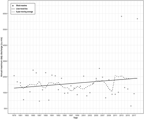
Thus, the MK test, the linear trend curve and the 5-year moving average curve depict the inclusive trend and the variations present in the block maxima time series, which confirms the non-stationary behaviour of the streamflow block maxima data.

5.1.2 Change point analysis

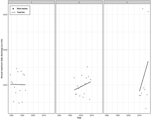
The 5-year moving average curve (Fig. 5) shows the evident variations in the block maxima time series. The 5-year moving average curve changed direction in the years 1994, 1998, 2007, and 2010 compared with the linear trend line of streamflow block maxima (Fig. 5); this indicates a change in the trend of the time series and thus put forward the possibility of multiple change points. Therefore, in this study, change point analysis was carried out using the PELT test, E-divisive method, Pettit test, Pruned objective via E-statistic, and pruned objective via Kolmogorov-Smirnov statistic. The results of these tests were compared to each other and with the moving average curve to obtain the optimum change points and to eliminate false positives. The change points of streamflow block maxima are shown in Table 2. The results showed that the years 1994 and 2010 were common change points according to many tests, with a significance level of 95%. The E-divisive change point test registered the same years (1994 and 2010), and it was concluded that this test is most appropriate of all, as it did not give any false change points. Thus, for streamflow block maxima, 1994 and 2010 were considered as the possible locations of change points.

Table 2. Change points of streamflow block maxima of Periyar River from 1979 to 2018

Change point test	Change points of streamflow block maxima
PELT	2010, 2013, 2017
E-divisive	1994, 2010
Pettitt	1994
Pruned objective via E-statistic	1994, 2004, 2010
Pruned objective via Kolmogorov-Smirnov statistic	1994, 2001, 2010

Adding change points of streamflow block maxima at 1994 and 2010 divided the series into three parts. To observe the linear inter-annual trend of the streamflow block maxima of each part, the linear trend of each part is shown in Fig. 6. From 1979 to 1993, data points were found to follow a falling trend with r = −0.016, then from 1994 to 2009 a rising trend was observed with r = 0.27, and then from 2010 to 2018 a steeply rising trend was observed with r = 0.28. The “r” values of linear trends are not significant due to the assumption of linearity; however, changing trends validate the chosen change points and confirm the non-stationarity of the block maxima time series.

Figure 6. Distribution and trend of streamflow block maxima time series with the change points at 1994 and 2010. The trend line is shown as a solid line

5.2 Non-stationary bivariate flood frequency analysis

The trend test and change point tests indicated the presence of non-stationarity, but to confirm the need for non-stationary flood frequency analysis, other field evidence is needed, which may help to characterize the presence of non-stationarity. Thus, the streamflow block maxima were modelled by GEV distribution, with time, AP, and URBEXT as covariates. The estimated parameters, negative log-likelihood estimates (–2log(L)), and AIC values of the models are shown in Table 3.

Table 3. Estimate of location, shape and scale parameters, negative log-likelihood and AIC values of the models

Model name			Model parameters					−2log(L)	AIC
	µo	µ1	µ2	σ o	σ 1	σ 2	ξ
M0	108.22	-	-	615.51	-	-	0.15	324.40	654.80
Mt1	1610.96	−2.88	-	602.33	-	-	0.17	324.19	656.37
Mt2	1589.80	-	-	6.19	0.01	-	0.14	323.50	654.99
Mt3	1589.80	1.18		6.18	0.01	-	0.1	323.47	656.94
Mp1	1463.70	0.07	-	642.03	-	-	0.17	323.13	654.27
Mp2	1643.70	-	-	7.58	−0.004	-	0.32	323.4	654.8
Mp3	1589.7	0.05	-	7.61	−0.004	-	0.31	322.45	654.91
Mu1	1740.67	−88.67	-	603.96	-	-	0.18	323.80	655.60
Mu2	1589.81	-	-	5.89	0.31	-	0.12	322.85	653.70
Mu3	1599.59	15.87	-	5.88	0.32	-	0.10	322.77	655.54
Mpu1	1421.37	0.20	−238.60	565.83	-	-	0.20	320.40	650.80
Mpu2	1677.2	-	-	6.6	−0.002	0.28	0.19	322.43	654.87
Mpu3	1290.06	0.22	−1882.96	6.73	−0.001	0.08	0.27	321.31	652.62

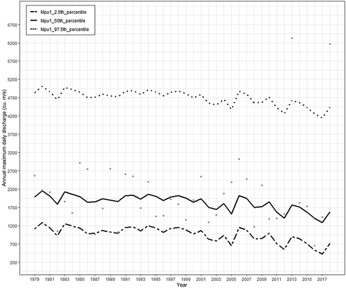
The model M_pu1, which was built with AP and URBEXT as a covariate of the location parameter, showed the maximum negative log-likelihood and minimum AIC value, and thus was considered the optimal model for the flood frequency analysis of non-stationary streamflow block maxima. The location parameter obtained for this model was µ = [1 421.37 + (0.20 × AP)−(238.60 × URBEXT)], the scale parameter was 565.83, and the shape parameter was 0.20. The appropriateness of the model M_pu1 suggests that the streamflow block maxima series of the study area is dependent on AP and URBEXT. The percentile plot of the model M_pu1, shown in Fig. 7, indicates that the majority of the streamflow block maxima data points are within the 2.5th and 97.5th percentiles, which indicates that the model captured the variability of data appropriately. The negative log-likelihood estimates and AIC values of the other models indicate that the existence of non-stationarity and the individual influence of time, AP, and URBEXT on streamflow block maxima was not substantial. Thus, it is important to analyse the non-stationary behaviour of streamflow data with the inclusion of natural and anthropogenic indicators for its flood frequency analysis.

Figure 7. Percentile plots showing 2.5th, 50th and 97.5th percentile values of non-stationary model with annual precipitation and urban extent as linear function of location parameter (black points are the streamflow block maxima values)

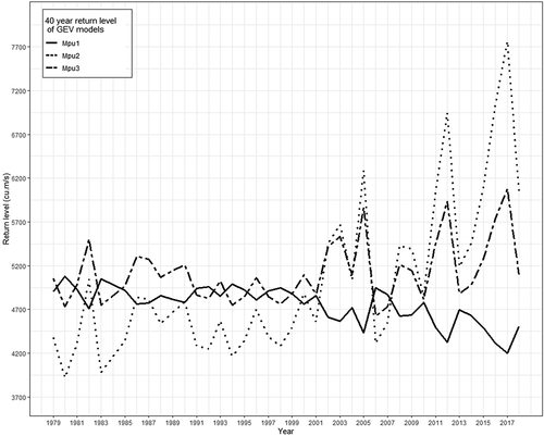
In this study, location and shape parameters were estimated using linear regression with the physical covariates (AP and URBEXT). The importance of estimating both parameters can be explained by Fig. 8, which shows the 40-year return levels estimated by the models M_pu1, M_pu2, and M_pu3 (Table 3). The return levels of M_pu2 and M_pu3 rise from 1979 to 2018 and their respective levels contradict the levels estimated by model M_pu1. For example, the return level of the year 1982 is higher than that of the year 1981 for models M_pu2 and M_pu3, but in the model M_pu1 the return level of the year 1982 is lower than that of the year 1981; similar observations are found for other years also. This illustrates the significance of modelling both location and shape parameters for non-stationary flood frequency analysis. If only the location parameter or only the scale parameter is modelled, the flood levels can fluctuate drastically; therefore, it is important to consider all possible combinations to obtain the optimal model. Sraj et al. (2015) modelled the non-stationary GEV distribution with only the location parameter as a function of annual precipitation, which may limit the scope of flood frequency analysis.

Figure 8. Comparison of 40-year return levels of non-stationary models built with annual precipitation and urban extent as linear function of (i) location parameter, (ii) scale parameter and (iii) location and scale parameter both

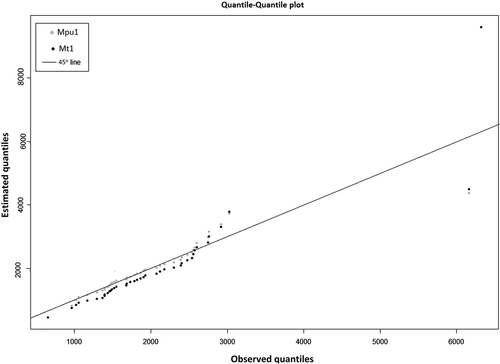
Many studies (e.g. Serago and Vogel 2018, Kang et al. 2020) conducted non-stationary flood frequency analysis with time as a covariate, considering it a proxy for all changing physical phenomena. To understand the rationality of this assumption, the model built with time (covariate) being linearly dependent on the location parameter (M_t1) and the optimal model M_pu1 are compared using the quantile-quantile (QQ) plot (Fig. 9). The QQ plot shows that M_pu1 is a good fit for the streamflow block maxima data, as the plot is moving close to the 45° line, except at the upper right corner. In contrast, the QQ plot of M_t1 shows deviations compared to that of M_pu1, thus it can be concluded that M_pu1 is a better fit and time alone is not capable of explaining the non-stationarity.

Figure 9. Quantile-quantile plot of non-stationary model built with (i) annual precipitation and urban extent as linear function of location parameter and (ii) time as linear function of location parameter

To understand the distinctions in flood frequency analysis caused by the assumption of stationarity and by considering only time as the covariate of the non-stationarity, the 2-year and 40-year return levels of models M₀, M_t1, and M_pu1 were compared and are shown in Figs 10 and 11. The 2-year return levels represent the median of the model (Sraj et al. 2015). The 2-year return level plot shows that the return levels of the stationary model are lower than that of M_pu1 until 2001, thus the median of the streamflow block maxima has been underestimated by the stationary model until 2001. After the year 2001, in contrast, the 2-year return levels or the median of the streamflow block maxima are mostly overestimated by the stationary model. This disparity represents the extent of error that may arise due to the involvement of stationarity for the flood frequency analysis. The 2-year return levels of model M_t1 show that the respective return levels have been underestimated compared to those of M_pu1 in almost every year, which indicates the significance of physical covariates for the non-stationary flood frequency analysis.

Figure 10. Comparison of 2-year return levels of stationary and non-stationary model built with (i) annual precipitation and urban extent as linear function of location parameter and (ii) time as linear function of location parameter

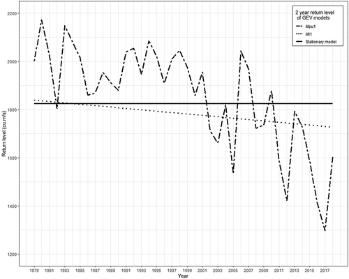
Figure 11. Comparison of 40-year return levels of stationary and non-stationary model built with (i) annual precipitation and urban extent as linear function of location parameter and (ii) time as linear function of location parameter

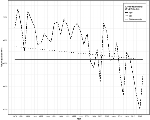
The 40-year return level plot (Fig. 11) shows higher levels for the model M_pu1 than for M₀ and M_t1 in most years. The estimation of the return period using the traditional methods assumes that the hydrologic events are stationary and the occurrence of events is independent or weakly dependent, thus in the non-stationary flood frequency analysis, these traditional concepts of return period become unclear (Cooley 2013). The two explanations of the return period proposed for non-stationary return period calculation are expected waiting time (EWT) and the expected number of events (ENE). The EWT denotes the time (T) in which the flood exceeding the design flood will occur for the first time (Cooley 2013, Salas and Obeysekera 2014), and the ENE represents the frequency of floods exceeding the design flood with time, under non-stationary regimes (Cooley 2013). In this study, ENE has been employed to obtain the non-stationary return period, according to which the return level corresponding to the 20-year and 40-year return period of the stationary model (M₀) was 16-year and 28-year respectively for the non-stationary model (M_pu1). A hydraulic structure constructed in the Periyar River basin under the assumption of stationarity with a design life of 40 years has a design life of only 28 years under the influence of climate change and anthropogenic interventions. Thus, water resources planning decisions taken with the assumption of stationarity may be unsafe, and to ensure the required level of protection under the influence of physical phenomena, the design discharge levels need to be altered.

Few studies have been conducted in India for non-stationary flood frequency analysis (Singh et al. 2015, Ray and Goel 2019, Sen et al. 2020), and those that have been carried out support the need to reconsider the assumption of stationarity. A framework that can perform both detection and attribution of non-stationarity is vital for the regions that are facing rapid urbanization and extreme flood events. This study shows that the impact of climate change and anthropogenic activities have introduced non-stationarity into the annual maximum daily discharge of the Periyar River basin. A similar study should be conducted for different regions of India based on the dominant physical phenomena, for safe water resources planning and management.

6 Conclusion

This study developed a non-stationary GEV model for flood frequency analysis in the Periyar River basin. Block maxima of the annual maximum daily discharge data from the period 1979 to 2018 of Periyar River were taken for the analysis. The non-parametric MK trend test and the E-divisive change point test confirmed the existence of non-stationarity in the streamflow block maxima time series. For the non-stationary flood frequency, the location and scale parameters of the GEV distribution were modelled by performing linear regression with annual precipitation, urban extent, and time, although future research could consider other extreme value theories, such as the metastatistical extreme value (MEV) approach (Marani and Ignaccolo 2015), to extend the scope of the study. According to the negative log-likelihood estimate and AIC value, the non-stationary GEV distribution modelled with annual precipitation and urban extent as a linear function of the location parameter was found to be more appropriate than the other models, which explains the influence of both climate change and anthropogenic activities on the non-stationarity of streamflow data. The comparison of the chosen non-stationary model with the stationary model showed that the return level corresponding to the 20-year and 40-year return period of the stationary model (M₀) was 16- years and 28 years, respectively, for the non-stationary model (M_pu1). Thus, the assumption of stationarity may lead to the unsafe design of structures. This study provides insights into the non-stationarity in Periyar annual maximum daily discharge data, which can lead to better flood frequency analysis and a better understanding of floods in this region. The methodology proposed in this study can be substituted for the complex frameworks that require exhaustive understanding to avoid incorrect conclusions. Thus, through this methodology, detection and attribution of non-stationarity can be accomplished for effective flood frequency analysis of different regions.

Acknowledgements

The authors are thankful to the Central Water Commission for providing the discharge data and rainfall data for Periyar River basin.

Disclosure statement

No potential conflict of interest was reported by the authors.

Additional information

Funding

This work was supported by the Programmatic Cooperation between the Directorate-General for International Cooperation (DGIS) of the Dutch Ministry of Foreign Affairs and IHE Delft in the period 2016–2023, also called DUPC2 [DUPC2]; and by the United Nations Educational, Scientific and Cultural Organization – Institute for Water Education (IHE Delft) [2019/089/108483/EWH (GRACERS project)].

References

- Akaike, H., 1974. A new look at the statistical model identification. IEEE Transactions on Automatic Control, 19 (6), 716–723. doi:https://doi.org/10.1109/TAC.1974.1100705.
- Amritanand, S., Anand, S., and Amritesh, A.R., 2020. Dynamic and time critical emergency management for level three disaster: a case study analysis of Kerala Floods 2018. In: Proceedings of the 21st international conference on distributed computing and networking, Kolkata, India, 1–6.
- Central Water Commission, 2018. Annual report 2018-19. New Delhi: Central Water Commission, Ministry of Water Resources, Government of India.
- Chinnasamy, P., Honap, V.U., and Maske, A.B., 2020. Impact of 2018 Kerala floods on soil erosion: need for post-disaster soil management. Journal of the Indian Society of Remote Sensing, 48 (10), 1373–1388. doi:https://doi.org/10.1007/s12524-020-01162-z
- Chinnasamy, P., Maske, A.B., Honap, V., Chaudhary, S., and Agoramoorthy, G., 2021. Sustainable development of water resources in marginalised semi‐arid regions of India: Case study of Dahod in Gujarat, India. In: Natural Resources Forum. Oxford, UK: Blackwell Publishing Ltd. doi: https://doi.org/10.1111/1477-8947.12217
- Chinnasamy, P., and Sood, A., 2020. Estimation of sediment load for Himalayan Rivers: Case study of Kaligandaki in Nepal. Journal of Earth System Science, 129 (1), 1–18. doi:https://doi.org/10.1007/s12040-020-01437-6
- Coles, S., 2001. An introduction to statistical modeling of extreme values, Vol. 208. London: Springer.
- Condon, L.E., Gangopadhyay, S., and Pruitt, T., 2015. Climate change and non-stationary flood risk for the upper Truckee River basin. Hydrology and Earth System Sciences, 19 (1), 159. doi:https://doi.org/10.5194/hess-19-159-2015.
- Cooley, D., 2013. Return periods and return levels under climate change. In: A. AghaKouchak, D. Easterling, and K. Hsu, eds. Extremes in a changing climate: Detection, analysis and uncertainty. New York: Springer, 97-114.
- Du, T., et al., 2015. Return period and risk analysis of nonstationary low-flow series under climate change. Journal of Hydrology, 527, 234–250. doi:https://doi.org/10.1016/j.jhydrol.2015.04.041
- Faulkner, D., et al., 2020. Can we still predict the future from the past? Implementing non‐stationary flood frequency analysis in the UK. Journal of Flood Risk Management, 13 (1), 12582. doi:https://doi.org/10.1111/jfr3.12582.
- Fisher, R.A., 1920. A mathematical examination of the methods of determining the accuracy of an observation by the mean error, and by the mean square error. Monthly Notices of the Royal Astronomical Society, 80, 758–770. doi:https://doi.org/10.1093/mnras/80.8.758
- Gado, T.A., 2016. An at-site flood estimation method in the context of nonstationarity II. Statistical analysis of floods in Quebec. Journal of Hydrology, 535, 722–736. doi:https://doi.org/10.1016/j.jhydrol.2015.12.064
- Gilleland, E. and Katz, R.W., 2016. extRemes 2.0: an extreme value analysis package in R. Journal of Statistical Software, 72 (1), 1–39. doi:https://doi.org/10.18637/jss.v072.i08.
- Gumbel, E.J., 1958. Statistics of Extremes. New York: Columbia University Press.
- Hamed, K.H. and Rao, A.R., 1998. A modified Mann-Kendall trend test for autocorrelated data. Journal of Hydrology, 204 (1–4), 182–196. doi:https://doi.org/10.1016/S0022-1694(97)00125-X.
- Haynes, K., et al., 2016. Changepoint. np: methods for nonparametric changepoint detection (R package version 0.0), 2.
- Haynes, K., Eckley, I.A., and Fearnhead, P., 2017. Computationally efficient changepoint detection for a range of penalties. Journal of Computational and Graphical Statistics, 26 (1), 134–143. doi:https://doi.org/10.1080/10618600.2015.1116445.
- Henderson, T.C., et al., Jul 2009. Automatic segmentation of semantic classes in raster map images. In: Eighth IAPR international workshop on graphics recognition GREC 2009, La Rochelle, France, 17.
- Hunt, K.M. and Menon, A., 2020. The 2018 Kerala floods: a climate change perspective. Climate Dynamics, 54 (3), 2433–2446. doi:https://doi.org/10.1007/s00382-020-05123-7
- India-Water Resources Information System, India-WRIS, viewed July 2020, www.india-wris.nrsc.gov.in.
- Jaiswal, R.K., Lohani, A.K., and Tiwari, H.L., 2015. Statistical analysis for change detection and trend assessment in climatological parameters. Environmental Processes, 2 (4), 729–749.
- James, N.A. and Matteson, D.S., 2015. ecp: an R package for nonparametric multiple change point analysis of multivariate data. Journal of Statistical Software, 62 (7), 1–25.
- Kang, L., et al., 2020. Evaluation of return period and risk in bivariate non-stationary flood frequency analysis. Water, 11 (1), 79. doi:https://doi.org/10.3390/w11010079.
- Killick, R. and Eckley, I., 2014. changepoint: an R package for changepoint analysis. Journal of Statistical Software, 58 (3), 1–19. doi:https://doi.org/10.18637/jss.v058.i03.
- Lal, P., et al., 2020. Evaluating the 2018 extreme flood hazard events in Kerala, India. Remote Sensing Letters, 11 (5), 436–445. doi:https://doi.org/10.1080/2150704X.2020.1730468.
- Machiwal, D. and Jha, M.K., 2009. Time series analysis of hydrologic data for water resources planning and management: a review. Journal of Hydrology and Hydromechanics, 54 (3), 237–257.
- Madhusoodanan, M.S., 2018. Dynamical downscaling of regional climate: Simulation of extreme rainfall events and their impacts over the state of Kerala in the near-future. Amritapuri: Amrita Vishwa Vidyapeetham. Available from: https://www.google.com/url?sa=t&rct=j&q=&esrc=s&source=web&cd=&ved=2ahUKEwjEq4HG3-zyAhWBcn0KHaEaANYQFnoECAQQAQ&url=https%3A%2F%2Fsdma.kerala.gov.in%2Fwp-content%2Fuploads%2F2019%2F08%2FKSDMA_Project_report_2017-2018.pdf&usg=AOvVaw3uEVQEcPyRwqSdfn8Z9Cpr [Accessed 4 November 2020].
- Mann, H.B., 1945. Nonparametric tests against trend. Econometrica: Journal of the Econometric Society, 13, 245–259. doi:https://doi.org/10.2307/1907187
- Mann, H.B. and Whitney, D.R., 1947. On a test of whether one of two random variables is stochastically larger than the other. The Annals of Mathematical Statistics, 18, 50–60. doi:https://doi.org/10.1214/aoms/1177730491
- Marani, M. and Ignaccolo, M., 2015. A metastatistical approach to rainfall extremes. Advances in Water Resources, 79, 121–126. doi:https://doi.org/10.1016/j.advwatres.2015.03.001
- Matteson, D.S. and James, N.A., 2014. A nonparametric approach for multiple change point analysis of multivariate data. Journal of the American Statistical Association, 109 (505), 334–345.
- Merz, B., et al., 2012. HESS Opinions’ More efforts and scientific rigour are needed to attribute trends in flood time series’. Hydrology and Earth System Sciences, 16 (5), 1379–1387. doi:https://doi.org/10.5194/hess-16-1379-2012.
- Pettitt, A.N., 1979. A non‐parametric approach to the change‐point problem. Journal of the Royal Statistical Society: Series C (Applied Statistics), 28 (2), 126–135.
- Pohlert, T., 2020. trend: non-parametric trend tests and change-point detection (Version 1.1.2).
- Priju, C.P., et al., 2018. Delineation of paleochannels in Periyar River Basin of Kerala using remote sensing and electrical resistivity methods. In: R.N. Yadava, S. Yadav, V.P. Singh, eds. Hydrologic modeling. Singapore: Springer, 391–400.
- Prosdocimi, I., Kjeldsen, T.R., and Miller, J.D., 2015. Detection and attribution of urbanization effect on flood extremes using nonstationary flood‐frequency models. Water Resources Research, 51 (6), 4244–4262. doi:https://doi.org/10.1002/2015WR017065.
- Ray, L.K. and Goel, N.K., 2019. Flood frequency analysis of Narmada River Basin in India under nonstationary condition. Journal of Hydrologic Engineering, 24 (8), 05019018. doi:https://doi.org/10.1061/(ASCE)HE.1943-5584.0001808.
- Rigby, R.A. and Stasinopoulos, D.M., 2005. Generalized additive models for location, scale and shape. Journal of the Royal Statistical Society: Series C (Applied Statistics), 54 (3), 507–554.
- Ryberg, K.R., Hodgkins, G.A., and Dudley, R.W., 2020. Change points in annual peak streamflows: method comparisons and historical change points in the United States. Journal of Hydrology, 583, 124307. doi:https://doi.org/10.1016/j.jhydrol.2019.124307
- Salas, J.D. and Obeysekera, J., 2014. Revisiting the concepts of return period and risk for nonstationary hydrologic extreme events. Journal of Hydrologic Engineering, 19 (3), 554–568. doi:https://doi.org/10.1061/(ASCE)HE.1943-5584.0000820.
- Salas, J.D., Obeysekera, J., and Vogel, R.M., 2018. Techniques for assessing water infrastructure for nonstationary extreme events: a review. Hydrological Sciences Journal, 63 (3), 325–352. doi:https://doi.org/10.1080/02626667.2018.1426858.
- Sen, S., He, J., and Kasiviswanathan, K.S., 2020. Uncertainty quantification using the particle filter for non-stationary hydrological frequency analysis. Journal of Hydrology, 584, 124666. doi:https://doi.org/10.1016/j.jhydrol.2020.124666
- Serago, J.M. and Vogel, R.M., 2018. Parsimonious nonstationary flood frequency analysis. Advances in Water Resources, 112, 1–16. doi:https://doi.org/10.1016/j.advwatres.2017.11.026
- Serinaldi, F. and Kilsby, C.G., 2015. Stationarity is undead: uncertainty dominates the distribution of extremes. Advances in Water Resources, 77, 17–36. doi:https://doi.org/10.1016/j.advwatres.2014.12.013
- Singh, J., et al., 2015. A framework for investigating the diagnostic trend in stationary and nonstationary flood frequency analyses under changing climate. Journal of Climate Change, 1 (1, 2), 47–65. doi:https://doi.org/10.3233/JCC-150004.
- Sivakumar, B., 2016. Chaos in hydrology: bridging determinism and stochasticity. Dordrecht, Netherlands: Springer.
- Sraj, M., Bezak, N., and Brilly, M., 2015. Bivariate flood frequency analysis using the copula function: a case study of the Litija station on the Sava River. Hydrological Processes, 29 (2), 225–238. doi:https://doi.org/10.1002/hyp.10145.
- Sudheer, K.P., et al., 2019. Role of dams on the floods of August 2018 in Periyar River Basin, Kerala. Current Science, 116 (5), 780– 794.
- Um, M.J., et al., 2017. Modeling nonstationary extreme value distributions with nonlinear functions: an application using multiple precipitation projections for US cities. Journal of Hydrology, 552, 396–406. doi:https://doi.org/10.1016/j.jhydrol.2017.07.007
- Wambui, G.D., Waititu, G.A., and Wanjoya, A., 2015. The power of the pruned exact linear time (PELT) test in multiple changepoint detection. American Journal of Theoretical and Applied Statistics, 4 (6), 581. doi:https://doi.org/10.11648/j.ajtas.20150406.30.
- Yan, L., et al., 2017. Comparison of four nonstationary hydrologic design methods for changing environment. Journal of Hydrology, 551, 132–150. doi:https://doi.org/10.1016/j.jhydrol.2017.06.001
- Yee, T.W. and Stephenson, A.G., 2007. Vector generalized linear and additive extreme value models. Extremes, 10 (1–2), 1–19. doi:https://doi.org/10.1007/s10687-007-0032-4.
- Yee, T.W. and Wild, C.J., 1996. Vector generalized additive models. Journal of the Royal Statistical Society: Series B (Methodological), 58 (3), 481–493.
- Yue, S., Pilon, P., and Phinney, B.O.B., 2003. Canadian streamflow trend detection: impacts of serial and cross-correlation. Hydrological Sciences Journal, 48 (1), 51–63. doi:https://doi.org/10.1623/hysj.48.1.51.43478.
- Zhang, W., James, N.A., and Matteson, D.S., Nov 2017. Pruning and nonparametric multiple change point detection. In: 2017 IEEE International Conference on Data Mining Workshops (ICDMW). New Orleans, LA: IEEE, 288–295.
- Zou, C., et al., 2014. Nonparametric maximum likelihood approach to multiple change-point problems. The Annals of Statistics, 42 (3), 970–1002. doi:https://doi.org/10.1214/14-AOS1210.