Daily scale river flow simulation: hybridized fuzzy logic model with metaheuristic algorithms

ABSTRACT

Novel data-intelligence models developed through hybridization of an adaptive neuro-fuzzy inference system (ANFIS) with different metaheuristic algorithms, namely grey wolf optimizer (GWO), particle swarm optimizer (PSO) and whale optimization algorithm (WOA), are proposed for daily river flow prediction of the Taleghan River, which is the major source of potable water for Tehran, the capital of Iran. Gamma test (GT) was used for the determination of input variables for the models. The ANFIS-WOA model was found to exhibit the best performance in prediction of river flow according to root mean square error (RMSE ≈ 3.75 m³.s⁻¹) and Nash-Sutcliffe efficiency (NSE ≈ 0.93). It improved the prediction performance of the classical ANFIS model by 6.5%. The convergence speed of ANFIS-WOA was also found to be higher compared to other hybrid models. The success of the ANFIS-WOA model indicates its potential for use in the simulation of highly nonlinear daily rainfall–runoff relationships.

KEYWORDS:

• metaheuristic algorithms
• ANFIS
• river flow prediction
• catchment management
• hybrid model

Editor S. Archfield Associate Editor N. Ilich

1 Introduction

Reliable prediction of daily river flow is still a research challenge for resolving various hydrological problems including water resource optimization, determining permitted release rate of pollutants, flood hazard forecasting and drought warning (Rezaie-Balf et al. 2017). For rivers with a dam in the outlet, prediction of inlet flow to the dam is important for regulating dam outlet valves. The Taleghan River basin in the northwest of Iran has a strategic position due to its proximity to the capital. The Taleghan River is the source of potable water for Tehran, the capital of Iran. Furthermore, it is the major source of irrigation for Qazvin plain downstream of the Taleghan dam. Therefore, predicting the daily flow of Talenghan River is highly important for ensuring the water security of the national capital of Iran and agricultural activity in the region.

Accurate prediction of river flows for shorter time intervals is always a challenge for hydrologists (Al-Sudani et al. 2019, Yaseen et al. 2020). Over the last few decades, several theory-driven (e.g. conceptual hydrological models) and machine learning (ML) algorithms have been adopted and extended for runoff modelling (Solomatine and Dulal 2003, Rajurkar et al. 2004, Kostić et al. 2016, Li et al. 2016. Process-driven models, e.g. Identification of unit Hydrographs and Component flows from Rainfall, Evaporation and Streamflow data (IHACRES) (Croke et al. 2006), Hydrological Simulation Program – FORTRAN (HSPF) (Bicknell et al. 1997), Soil and Water Assessment Tool (SWAT) (Arnold et al. 1998) etc., are useful for understanding the physically-based hydrological processes in a watershed. However, the main constraint of such models is their extensive data requirements, which restricts their applicability to only intensively monitored watersheds. Furthermore, such models are often not suitable for accurate prediction of river flow at a specific location with affordable time and cost.

ML models can simulate hydrological processes without requiring any understanding of the physical mechanism of the watershed runoff generation. They can be simply constructed based on hydrometeorological input–output data series (Devia et al. 2015, Rezaie-Balf et al. 2017). In comparison with theory-driven models, ML models need fewer variables as input and, consequently, the data requirement of these models is significantly less than that of the theory-driven models. Several ML models have been developed, such as support vector machines (SVM), artificial neural network (ANN), adaptive neuro-fuzzy inference system (ANFIS), genetic programming (GP), M5 model trees (M5Tree) and classification and regression trees (CART) (Anctil et al. 2004, Solomatine and Xue 2004, Turan and Yurdusev 2009, Napolitano et al. 2011, Tiwari et al. 2013, Elsafi 2014, Chen et al. 2015, Zhang et al. 2018, Yang et al. 2019, Afan et al. 2020. These models have been extensively employed in hydro-environmental studies including precise prediction of river flow.

Despite the widespread use of ML models in hydrology, there are a few major drawbacks of ML models. The prediction capability of ML models relies heavily upon the tuning of their internal parameters (Chen et al. 2017), which are also known as hyper-parameters (Yaseen et al. 2019, Memarzadeh et al. 2020). Accurate tuning of internal parameters is required for robust learning of the prediction matrix (Qi et al. 2020). Hence, optimization of hyper-parameters is essential to improve the predictability of ML-based hydrological models. The most popular optimization procedure is the trial and error experiment; however, it is always time-consuming and often produces unrealistic predictions (Leuenberger et al. 2018). The issue of poor prediction becomes more severe in modelling highly nonlinear and nonstationary process, such as river flow simulation, which forces the modeller to make many attempts to achieve the desired results.

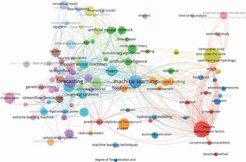
Among the ML models, ANFIS is one of the more effective models which has been extensively employed for hydrological simulation (Jacquin and Shamseldin 2009, Ghose et al. 2013, Roushangar et al. 2014). Learning the membership functions and adjustment of interconnections among the layers are the major challenges in developing an ANFIS model. Generally, a gradient descent approach is applied for optimization of ANFIS model parameters (Buragohain and Mahanta 2008), where the gradient is calculated in each iteration. The performance of this optimization is influenced by the initial conditions (Ewees and Elaziz 2018). Recent studies have shown the potential of metaheuristic optimization algorithms in the selection of optimal values for ML model internal parameters (Ewees and Elaziz 2018, Jaafari et al. 2019). For example, based on the reported visualization of the bibliometric network using the Scopus database search for the keywords “river flow” and “hybrid machine learning,” over 400 keywords appeared based on the cluster division using the VOSviewer algorithm (Fig. 1). These optimization algorithms can also be employed for automatic estimation of optimum ML model internal parameters to improve the model’s capability (Razavi Termeh et al. 2018).

Figure 1. The occurrence of major keywords reported in the literature, based on the Scopus database using VOSviewer algorithm for the keywords search “river flow hybrid machine learning models.”

Firat and Güngör (2007) employed ANFIS for daily runoff modelling in Great Menderes in west Turkey. They used cross-validation methods with four different calibration and validation datasets and finally constructed the model with the best calibration dataset. The results showed that ANFIS can simulate daily river flow accurately. Li et al. (2018) employed ANFIS for daily river flow simulation of a small forested basin in China and compared the results with SVM and ANN model outputs. All the models were calibrated and validated with wavelet de-noised data. They showed that the ANFIS model can better simulate the low flows compared to ANN and SVM. Several research investigations over the past five years also employed hybrid ML models for river flow simulation (Maroufpoor et al. 2019, Meshram et al. 2019, Rezaie-Balf et al. 2019, Farfán et al. 2020, Torabi et al. 2020). The studies demonstrated the feasibility of the hybridized ML models for simulating hydrological processes (Rajaee et al. 2019).

A number of biologically inspired metaheuristic algorithms have been developed in recent years to resolve complex optimization problems (Mirjalili and Lewis 2016). These prevalent nature-inspired metaheuristic algorithms include particle swarm optimization (PSO; Kennedy and Eberhart 1995), the grey wolf optimizer (GWO; Mirjalili et al. 2014), and the whale optimization algorithm (WOA; Mirjalili and Lewis 2016). The motivation for this study was to employ robust and reliable ML models for reliable hydrological simulation. Therefore, novel ANFIS models are proposed in this study through hybridization with three nature-inspired metaheuristic algorithms – GWO, WOA and PSO – to improve the predictive performance for daily river flow. The efficacy of the proposed hybrid models was evaluated through their application in the simulation of daily river flow in Taleghan River basin in the north of Iran. The superiority of the proposed models is evaluated by comparing them with multiple linear regression (MLR), basic ANFIS and CART models.

The article is organized as follows: Section 2 presents a brief explanation of the optimization algorithms and the predictive models. Section 3 presents information about the study area and data. The experimental results are presented in Section 4. Lastly, the conclusion drawn from the results is reported in Section 5.

2 Methodology and model development

2.1 Model input identification

Input selection and division of data for model calibration and validation are the major decisive factors for the construction of a reliable predictive model (Choubin and Malekian 2017, Bhagat et al. 2020). The inputs were selected with the gamma test (GT) approach, which uses the input variables most correlated with the output as the most suitable inputs (Moghaddamnia et al. 2009). In addition, M-test (Stefánsson et al. 1997) was considered to identify the optimal calibration and validation data division. The model that yields the least mean square error (MSE) was identified through optimization of the V ratio and gamma statistic (Г) (Končar 1997).

2.1.1 Gamma test (GT)

GT optimizes the searching process using gamma statistic (Г) (Stefánsson et al. 1997), V ratio and standard error. For every $x_i\left(1\le k\le p\right)$ , Г statistic is estimated from $N\left(i,k\right)$ which is the k^th $\left(1\le k\le p\right)$ closest neighbour of $x_{N\left(i,k\right)}$ . The Г statistic can be estimated from input variables:

(1) ${\mathrm{\partial }}_M\left(k\right)=\frac{1}{M}\sum _{i=1}^M{\left|x_{N\left(i,k\right)}-x_i\right|}^2\left(1\le k\le p\right)$(1)

where M corresponds to sample size and│ … │is the Euclidean distance, for which the Г statistic is calculated as:

(2) ${\gamma }_M\left(k\right)=\frac{1}{2M}\sum _{i=1}^M{\left|y_{N\left(i,k\right)}-y_i\right|}^2\left(1\le k\le p\right)$(2)

where $y_{N\left(i,k\right)}$ is the k^th closest neighbour of $x_i$ on the y-axis. The Г statistic is estimated by fitting a least squares regression line across (${\mathrm{\partial }}_M\left(k\right)$ , ${\gamma }_M\left(k\right)$) points:

(3) $\gamma =A\delta +\mathrm{\Gamma }$(3)

The point of intersection of the γ and y-axis denotes Г, for which the least MSE can be obtained by utilizing a nonlinear model (Evans and Jones 2002). To verify the results of GT, the V ratio (= Г/σ²(y)) was also estimated using the scale-variant noise estimate between 0 and 1 (Seifi and Riahi 2020), where σ²(y) corresponds to variance of y. For a given model, V ratio and Г values close to zero indicate the optimal combination of the selected model (Stefánsson et al. 1997).

2.1.2 M-test

The Г statistic can be optimized by running the M-test to distinguish the optimal data length required for calibration and validation of a given nonlinear model. M-test helps to detect the point beyond which the MSE of the calibration dataset is lower than Var (r) and the model leads to overfitting. The Г–based M-test was utilized to specify the optimal amount of data required for tuning the models. The point at which the M-curve is minimum and becomes stable defines the optimal size of the calibration dataset.

2.2 Model setup and optimization

2.2.1 Adaptative neuro-fuzzy inference system (ANFIS)

ANFIS (Jang 1993) is developed by taking the advantages of ANN and fuzzy logic for approximation of nonlinear functions. The ANFIS model takes the benefits of ANN’s learning capabilities to learn the “if-then” rules of Takagi-Sugeno (TS) fuzzy inference system (FIS). ANFIS consists of five layers with two inputs (x, y) and one output (f). The two generic “if-then” rules of the TS model are:

(4) $ifais{X}_{1}andbis{Y}_{1}then{f}_1=p_{1}a+q_{1}b+r_1$(4)

(5) $ifais{X}_{2}andbis{Y}_{2}then{f}_2=p_{2}a+q_{2}b+r_2$(5)

In Equations (4)(4) $ifais{X}_{1}andbis{Y}_{1}then{f}_1=p_{1}a+q_{1}b+r_1$(4) and (5(5) $ifais{X}_{2}andbis{Y}_{2}then{f}_2=p_{2}a+q_{2}b+r_2$(5) ), a and b explain the input vectors, f is defined as the output, X and Y are the membership values of the input, and p, q and r are premise constraints approximated by ANNs. The fuzzification of input variables is done in the first layer, the triggering levels of the rules are estimated in the second layer, the triggering levels are normalized in the third layer, and the outcomes of individual rules are transferred to the fourth layer and are finally aggregated in the fifth layer to provide the model output (Jaafari et al. 2019).

2.2.2 Grey wolf optimization (GWO) algorithm

The GWO (Mirjalili et al. 2014) is a nature-inspired swarm-based method that emulates the social hierarchy of wolves and their behaviour in approaching, encircling and attacking their prey (Faris et al. 2017). Each member in a grey wolf herd is grouped as α, β, δ and ω based on the effectiveness and decision-making power in the group. To address an optimization problem, the social behaviour of the grey wolves in hunting is modelled in a statistical framework in the GWO algorithm. The chasing approach of the grey wolves comprises three stages: tracking, encircling and attacking (Muro et al. 2011). These processes are organized by α, β and δ wolves, respectively (Dehghani et al. 2019). The ω wolves follow the α, β and δ wolves (Mirjalili et al. 2014). The optimum solution is α, while β, δ and ω are the next subsequent solutions in term of priority. In GWO iterations, the wolves evaluate the possible hunts and update their status according to their position. The encircling method can be represented as:

(6) $\vec{X}\left(t+1\right)={\vec{X}}_p\left(t\right)-\vec{A}\cdot \left|\vec{C}\cdot {\vec{X}}_p\left(t\right)-\vec{X}\left(t\right)\right|$(6)

In the above equation, t is the present iteration; ${\vec{X}}_p$ and $\vec{X}$ are the location vectors of the hunt and hunter (candidate solutions), respectively; and $\vec{A}=2\vec{a}.{\vec{r}}_1-\vec{a}$ and $\vec{C}=2.{\vec{r}}_2$ indicate coefficient vectors, with ${\vec{r}}_1$ and ${\vec{r}}_2$ being random vectors (ranging from 0 to 1) that allow the wolves to change their status in the hunt space. The magnitude of $\vec{a}$ is gradually decreased from 2 to 0 using the following equation:

(7) $a\left(t\right)=2-\frac{2t}{\sum t}$(7)

where $\sum t$ signifies the total number of iterations. During the search process, ω wolves update their status according to the best exploration factors i.e. α, β and δ, which are represented as:

(8) ${\vec{X}}_1={\vec{X}}_{\alpha }-{\vec{A}}_1|{\vec{C}}_1\cdot {\vec{X}}_{\alpha }-\vec{X}$(8)

(9) ${\vec{X}}_2={\vec{X}}_{\beta }-{\vec{A}}_2\cdot |{\vec{C}}_2\cdot {\vec{X}}_{\beta }-\vec{X}$(9)

(10) ${\vec{X}}_3={\vec{X}}_{\delta }-{\vec{A}}_3\left|{\vec{C}}_3\cdot {\vec{X}}_{\delta }-\vec{X}\right|$(10)

(11) $\vec{X}\left(t+1\right)=\frac{{\vec{X}}_1+{\vec{X}}_2+{\vec{X}}_3}{3}$(11)

2.2.3 Whale optimization algorithm (WOA)

The WOA (Mirjalili and Lewis 2016) algorithm was developed based on the bubble-net feeding behaviour of humpback whales (Watkins and Schevill 1979), where the targeted prey is defined as the optimum output. The locations of whales surrounding the target can be expressed as

(12) $\vec{X}\left(t+1\right)={\vec{X}}^{\ast }\left(t\right)-\vec{A}\cdot \left|\vec{C}{\vec{X}}^{\ast }\left(t\right)-\vec{X}\left(t\right)\right|$(12)

where $\vec{X}$ represents whale location vectors; X* is the position vector of the target, which changes according to the location of most suitable target; and $\vec{A}=2\vec{a}.\vec{r}-\vec{a}$ and $\vec{C}=2.\vec{r}$ represent coefficient vectors.

The bubble-net preying process comprises two steps: (i) decrease circling, which is realized by gradual reduction of $\vec{a}$ in the equation $\vec{A}=2\vec{a}.\vec{r}-\vec{a}$ . The magnitude of $\vec{A}$ decreases with the decrease of $\vec{a}$ ; (ii) spiral changes of location, which are implemented by emulating whales’ spiral movement around the prey by estimating the distance of prey (X*, Y*) from a whale (X, Y):

(13) $\vec{X}\left(t+1\right)={\vec{D}}^{\prime }{e}^{bl}\cdot \mathrm{c}\mathrm{o}\mathrm{s}\left(2\pi l\right)+{\vec{X}}^{\ast }\left(t\right)$(13)

where ${\vec{D}}^{\prime }=\left|{\vec{X}}^{\ast }\left(t\right)-\vec{X}\left(t\right)\right|$ is the distance of the prey from the i^th whale, b is a constant that can be utilized to describe the logarithmic helix-type movement, and l is a random value between −1 and 1. The decreasing encircling path of whales can be represented using Equation (14):

(14) $\vec{X}\left(t+1\right)=\left\{\begin{array}{ccc}{\vec{X}}^{\ast }\left(t\right)-\vec{A}\cdot \vec{D}& \mathrm{i}\mathrm{f}& p<0.5\\ {\vec{D}}^{\prime }{e}^{bl}\cdot \mathrm{c}\mathrm{o}\mathrm{s}\left(2\pi l\right)+{\vec{X}}^{\ast }\left(t\right)& \mathrm{i}\mathrm{f}& p\ge 0.5\end{array}\right.$(14)

where p ∈ [0,1] defines the likelihood of continuation of the encircling approach or switching to a reduced rotation path to change the whales’ position. In the searching stage, whales hunt in a random mode according to each other’s position (Mirjalili and Lewis 2016). Therefore, the whales change their position using a random search factor, as given below:

(15) $\vec{D}=\left|\vec{C}\cdot {\vec{X}}_{rand}-\vec{X}\right|$(15)

(16) $\vec{X}\left(t+1\right)={\vec{X}}_{\mathrm{r}\mathrm{a}\mathrm{n}\mathrm{d}}-\vec{A}\cdot \vec{D}$(16)

where ${\vec{X}}_{rand}$ is a random location that is decided based on the population. A detailed description of WOA can be found in Mirjalili and Lewis (2016).

2.2.4 Particle swarm optimization (PSO)

PSO (Kennedy and Eberhart 1995) is a metaheuristic algorithm that imitates the joint performance of animal groups such as birds and fishes (Assareh et al. 2010). In PSO, it is assumed that the search space is covered by creatures or particles. Each particle is positioned compared to the target. The particles change location and velocity according to existing conditions. The best particles in the group can be expressed as:

(17) $\begin{array}{rl}{V}_{id}^t& =w{V}_{id}^{t-1}+C_1{r}_1\left(P_{id}^t-x_{id}^t\right)+C_2{r}_2\left(P_{gd}^t-x_{id}^t\right),\\ d& =1,2,\dots ,D\end{array}$(17)

where $x_{id}^t$ and $V_{id}^t$ are the position and velocity, respectively, of a particle having id = 1, …, D in iteration t; $P_{id}^t$ is the best location of a particle id = 1, …, D in iteration t; $P_{gd}^t$ is the global best position of an article gd = 1, …, D in iteration t; w represents inertia weight; C₁ and C₂ are cognition and social learning factors; and r₁ and r₂ denote random values in a range of 0 to 1. The procedure used for implementation of PSO is demonstrated in Fig. 2.

Figure 2. Flow diagram showing the procedure used for the development of meta-optimized models for river flow simulation

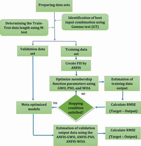
2.3 Model development

The procedure used for model development is described in Fig. 3 using a flowchart. The performance of the ANFIS model in river flow simulation was improved by optimizing the parameters of its membership function and the weights of the layers’ interconnections using metaheuristic algorithms.

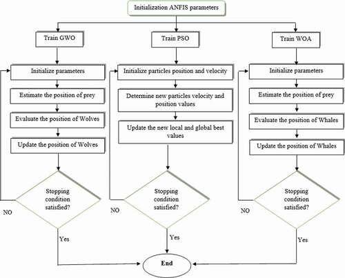
Figure 3. Flowchart of the applied metaheuristic algorithms (AWO, PSO and WOA)

2.3.1 The proposed hybrid models

The flowchart in Fig. 2 shows the procedure used for implementation of hybrid models. The input dataset was first normalized and then the GT algorithm, based on the gamma statistic and V ratio, was employed to identify the strongest model for daily scale river flow simulation. The model with the lowest gamma and V ratio values is considered the most suitable model for river flow simulation. The M-test is then applied to optimize the calibration and validation data length for the chosen model. The FIS is generated using the calibration dataset, and the parameters of the membership function are optimized using GWO, PSO and WOA. For statistical reasons and owing to the different results expected for each trial run, all the results were calculated based on the average of 30 independent runs for each model. The proposed meta-optimized models are, finally, employed for river flow simulation and the performance is evaluated using the commonly used metrics, root mean square error (RMSE), coefficient of determination (R²), Nash-Sutcliffe efficiency (NSE; Nash and Sutcliffe 1970), Kling-Gupta efficiency (KGE; Gupta et al. 2009) and analysis of variance (ANOVA). All experiments for identifying the most robust model and appropriate calibration and validation data division were conducted using the Wingamma software package. The proposed hybrid models were developed using Matlab 2014b on a computer with a Core i7 processor and 8 GB RAM.

2.3.2 Data normalization

Data are normalized to convert them into the range of −1 to +1 using Equation (18)(18) $Z=\frac{2\ast \left(X_i-X_{min}\right)}{\left(X_{max}-X_{min}\right)}-1$(18) (Khosravi et al. 2018):

(18) $Z=\frac{2\ast \left(X_i-X_{min}\right)}{\left(X_{max}-X_{min}\right)}-1$(18)

where Z is the standardized data in the range of −1 to +1, $X_i$ is the actual data and $X_{min}$ and $X_{max}$ represent the minimum and maximum of the actual data, respectively.

2.3.3 Model evaluation

Various performance evaluation criteria – R², KGE, NSE and RMSE – were utilized to evaluate the simulated results of each model, which are illustrated in Equations (19)(19) ${\mathrm{R}}^2={\left(\frac{{\sum }_{i=1}^N\left(O_i-\bar{O}\right)\left(P_i-\bar{P}\right)}{\sqrt{{\sum }_{i=1}^N{\left(O_i-\bar{O}\right)}^2{\sum }_{i=1}^N{\left(P_i-\bar{P}\right)}^2}}\right)}^2$(19) to (22) (Tiyasha et al. 2020):

(19) ${\mathrm{R}}^2={\left(\frac{{\sum }_{i=1}^N\left(O_i-\bar{O}\right)\left(P_i-\bar{P}\right)}{\sqrt{{\sum }_{i=1}^N{\left(O_i-\bar{O}\right)}^2{\sum }_{i=1}^N{\left(P_i-\bar{P}\right)}^2}}\right)}^2$(19)

(20) $\mathrm{K}\mathrm{G}\mathrm{E}=1-\sqrt{{(\mathrm{c}\mathrm{c}-1)}^2}+(\alpha -1{)}^2+(\beta -1{)}^2$(20)

(21) $\mathrm{N}\mathrm{S}\mathrm{E}=1-\frac{{\sum }_{i=1}^N{\left(O_i-P_i\right)}^2}{{\sum }_{i=1}^n{\left(O_i-\bar{O}\right)}^2}$(21)

(22) $\mathrm{R}\mathrm{M}\mathrm{S}\mathrm{E}=\sqrt{\sum _{i=1}^N{\left({\mathrm{O}}_i-{\mathrm{P}}_i\right)}^2}$(22)

where N represents length of the evaluated data; $O_i$ and $P_i$ are the observed and simulated data, respectively;$\bar{O}$ and $\bar{P}$ define the mean values of $O_i$ and $P_i$ series; cc expresses the correlation coefficient between $O_i$ and $P_i$ series; α explains the variability of discharge series (the ratio of the standard deviation (SD) of $P_i$ to the SD of $O_i$); and β explains the ratio of $\bar{P}$ to $\bar{O}$ (Gupta et al. 2009). The model simulations can be judged very good if ${\mathrm{R}}^2$ > 0.7 (Ayele et al. 2017), KGE > 0.85 (Pechlivanidis et al. 2014), NSE > 0.9 (Ritter and Muñoz-Carpena 2013) and RMSE ≈ 0 (Moriasi et al. 2007).

3 Case study area and explanation of data

The study area for the current research is Taleghan River basin, situated in the southern valley of the Alborz mountain range, approximately 100 km from Tehran, the capital of Iran. Geographically, it is located between $36°5\prime$ and $36°23\prime$ N latitude and between $50°20\prime$ and $51°10\prime$ E longitude and covers an area of 800 km² (Fig. 4). The watershed has a mountainous topography and Mediterranean climate with an average altitude of 2753 m, mean temperature of 4.48°C and annual average precipitation of 701 mm (Dodangeh et al. 2017). Developing the best runoff simulation model for Taleghan basin is vital because the river basin is a major supplier of water to the Taleghan dam. The Taleghan dam supplies the water for irrigation of agricultural activities in downstream of the dam (Dodangeh et al. 2019). It also supplies water for power generation in the dam with a capacity of 17.8 megawatts. The Taleghan River is also the major source of potable water for Tehran.

Figure 4. Location of the Taleghan River basin in northern Iran

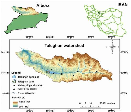
In the present study, hydrometeorological data recorded at six meteorological stations, one synoptic station and one hydrometric station for the period 1995–2005 were collected. For simulation of the river flow discharge on day t (Q_t), the initial input combination was constructed as follows: the air temperature on day t (T_t), the mean rainfall on day t (PG_t), the mean rainfall on the day before day t (PG_t-1), the mean rainfall on the two days before day t (PG_t-2), the discharge on the day before day t (Q_t-1), the discharge on the two days before day t (Q_t-2) and the discharge on the three days before day t (Q_t-3). The best input mask is decided using GT to simulate the river discharge at Galinak hydrometric station located at the watershed outlet. The daily input time series data for the period 23 September 1995 to 18 June 2003 was used for tuning the parameters of the investigated models. The calibrated models were validated for the period of 19 June 2003 to 22 September 2005.

4 Application results and discussion

4.1 Model identification

The prediction accuracy of ML algorithms significantly depends on the input combination used and the efficient size of the calibration data. The parameters estimated by GT are provided in Table 1. The simulations were run for 100 iterations, and in each iteration one or more input variables were masked. Table 2 outlines the results of GT after the first 10 iterations with the lowest gamma and V ratio statistics. The mask 1111101 yields the lowest gamma value ≈ 0.0063 and V ratio ≈ 0.007 and thus is the most suitable combination for river flow simulation. The PG_t and Q_t-1 were not masked in any of the 10 input combinations outlined in Table 2. This implies that these two variables are the most influential input variables for river flow simulation for day t (Q_t). The total travel time (time of concentration) of the watershed is 4.5 hours which justify the role of the current day precipitation (PG_t) for river flow simulation in the same day (Q_t).

Table 1. The parameter magnitudes for the applied gamma test (GT)

Parameter description	Parameter value
Population size	100
Mutation rate (MR)	0.05
Cross-over rate (CR)	0.5
Gradient fitness	0.1
Intercept fitness	1
Length fitness	0.1

Table 2. Determining the best input combination for DRSF simulation using the gamma test

Input combination	Gamma	Standard error	V ratio	Mask
Tt,PGt,PGt-2,PGt-1,Qt-1,Qt-3	0.0063	0.0007	0.025	1111101
PGt,PGt-2, PGt-1,Qt-1,Qt-3	0.0067	0.0009	0.026	0111101
Tt,PGt,PGt-2,PGt-1,Qt-1,Qt-2	0.007	0.001	0.028	1111110
Tt,PGt,PGt-1,Qt-1,Qt-2	0.007	0.001	0.028	1101110
Tt,PGt,PGt-2,PGt-1,Qt-1,Qt-2,Qt-3	0.007	0.001	0.029	1111111
PGt,PGt-2,PGt-1,Qt-1,Qt-2,Qt-3	0.007	0.0008	0.029	0111111
Tt,PGt,PGt-2,Qt-1,Qt-2,Qt-3	0.007	0.001	0.03	1110111
Tt,PGt,PGt-1,Qt-1,Qt-2,Qt-3	0.007	0.002	0.03	1101111
Tt,PGt,PGt-1,Qt-1,Qt-3	0.007	0.0006	0.03	1101101
Tt,PGt,PGt-2, PGt-1,Qt-1	0.007	0.0009	0.03	1111100

T(t), the air temperature on day t; PG_t, the mean rainfall on day t; PG_t-1, the mean rainfall in the 1 day prior to day t, PG_t-2, the mean rainfall in the 2 days prior to day t; Q_t-1, the discharge in the 1 day prior to day t; Q_t-2, the discharge in the 2 days prior to day t; Q_t-3, the discharge in the 3 days prior to day t.

4.2 Calibration data selection

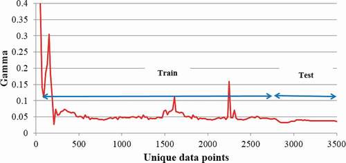
M-test was employed to determine the most efficient data period required for model calibration to achieve better simulation without encountering the overfitting problem. The proper length was assessed for the calibration and validation dataset to provide an accurate estimate of $\mathrm{\Gamma }$. Figure 5 depicts the M-curve values versus the data points for the best mask (1111101), identified in the previous section. The $\mathrm{\Gamma }$ value reached below 0.05 for 2800 data points and stabilized thereafter. Therefore, the calibration and validation data lengths were set at 80% and 20% for model development and validation, respectively.

Figure 5. Determination of proper train–test data division using M-test: gamma statistic vs. unique data points

4.3 ANFIS-WOA results

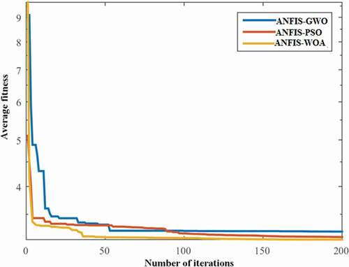
The ANFIS-WOA model calibration and validation were performed using historical daily river flow data. The calibrated hybrid model parameters are listed in Table 3; they were estimated for a population size of 25 and a maximum of 200 iterations. The performance of the investigated models in terms of statistical metrics is provided in Table 4. It was observed that the WOA algorithm improved the performance of the ANFIS model in terms of all statistics. The performance metrics of ANFIS-WOA were found to be much better (RMSE = 3.7, R² = 0.93 and KGE = 0.95) compared to the standalone ANFIS model (RMSE = 4.01, R² = 0.92 and KGE = 0.92). The WOA trainer was also found to outperform the other two metaheuristic trainers, GWO and PSO. The converging behaviours of the hybrid models are shown in Fig. 6. The convergence speeds of the metaheuristic optimization algorithms were measured based on MSE. The WOA algorithm exhibited the fastest convergence for the investigated dataset. Here, it can be seen that the WOA algorithm provided the best-optimized parameters for ANFIS compared to other two optimizers.

Table 3. Magnitudes of the essential parameters of the applied classical and hybrid predictive models

Algorithm	Parameter values
Anfis	Max epochs = 100, Error goal = 0, Initial step = 0.01, Decrease rate = 0.9
Anfis-GWO	$a=\mathrm{l}\mathrm{i}\mathrm{n}\mathrm{e}\mathrm{a}\mathrm{r}\mathrm{l}\mathrm{y}\mathrm{d}\mathrm{e}\mathrm{c}\mathrm{r}\mathrm{e}\mathrm{a}\mathrm{s}\mathrm{e}\mathrm{d}\mathrm{f}\mathrm{r}\mathrm{o}\mathrm{m}2\mathrm{t}\mathrm{o}0$ , A = $2\times a\times \left(rand\left(0,1\right)-a\right)$, C = $2\times rand\left(0,1\right)$
Anfis-PSO	Maximum inertia weight = 0.9, Minimum inertia weight = 0.2, Maximum velocity = 1.0, Minimum velocity = −1.0, Cognitive coefficient (C1) = 2, Cognitive coefficient (C2) = 2
Anfis-WOA	$a=\mathrm{l}\mathrm{i}\mathrm{n}\mathrm{e}\mathrm{a}\mathrm{r}\mathrm{l}\mathrm{y}\mathrm{d}\mathrm{e}\mathrm{c}\mathrm{r}\mathrm{e}\mathrm{a}\mathrm{s}\mathrm{e}\mathrm{d}\mathrm{f}\mathrm{r}\mathrm{o}\mathrm{m}2\mathrm{t}\mathrm{o}0$ , A = $2\times a\times \left(rand\left(0,1\right)-a\right)$ , Constant $b$ = 1, $l$ = $rand\left(-1,1\right)$, C = $2\times rand\left(0,1\right)$

Table 4. Performance evaluation of the applied meta-optimized and evolutionary-based models during training and validation stages

Stage	Predictive models	RMSE	R^2	KGE	NSE
Train	ANFIS-GWO	3.059	0.9526	0.9475	0.9521
	ANFIS-WOA	2.938	0.9559	0.9620	0.9558
	ANFIS-PSO	2.962	0.9554	0.9550	0.9551
	ANFIS	3.349	0.9426	0.9588	0.9426
	CART	3.522	0.9365	0.9544	0.9365
	MLR	3.34	0.9427	0.9589	0.9427
Validation	ANFIS-GWO	3.927	0.9281	0.9528	0.9281
	ANFIS-WOA	3.757	0.9343	0.9596	0.9342
	ANFIS-PSO	3.776	0.9337	0.9595	0.9335
	ANFIS	4.017	0.9250	0.9556	0.9248
	CART	5.57	0.8722	0.8773	0.8553
	MLR	4.05	0.9234	0.9511	0.9233

Note: Bold font indicates the best prediction results.

Figure 6. Convergence curves of optimization algorithms

4.4 ANFIS-PSO results

The performance metrics of the ANFIS-PSO model are provided in Table 4. ANFIS-PSO yielded statistical metric values of R² = 0.93, KGE = 0.95, and RMSE = 3.77. Similar to WOA, the PSO algorithm was able to enhance the efficiency of the ANFIS model in term of all statistics. Overall, the ANFIS-PSO model showed a very competitive performance in comparison with the other two metaheuristic optimizers. Results presented in Table 4 shows that PSO can be ranked as the second best optimizing algorithm after WOA. The comparison of the convergence behaviour of the PSO algorithm revealed a slightly slower convergence than the WOA algorithm, but a faster convergence than the GWO algorithm (Fig. 7).

4.5 ANFIS-GWO results

The performance of ANFIS-GWO also revealed an improvement in efficiency compared to the basic ANFIS model. The statistical metric values for ANFIS-GWO were found to be RMSE = 3.92, R² = 0.92 and KGE = 0.95. However, the ANFIS-GWO model showed the worst performance among the three hybrid models. The convergence curve of this model was also found to be the slowest (Fig. 6).

Figure 7 shows the daily river flow simulation for the validation phase using the proposed models. A comparison of the results presented in Table 4 and Figs 7 and Figs 8 reveals ANFIS-WOA is the best-performing model during both calibration (RMSE = 2.93, R² = 0.95, KGE = 0.96, NSE = 0.95) and validation (RMSE = 3.75, R² = 0.93, KGE = 0.95, NSE = 0.93). The ANFIS-PSO model (with RMSE = 3.76, R² = 0.93, KGE = 0.95, NSE = 0.93) followed by the ANFIS-GWO (with RMSE = 3.92, R² = 0.92, KGE = 0.95, NSE = 0.92) were ranked as second and third in terms of prediction accuracy. It is worth noting that all of the meta-heuristic optimization algorithms improved the performance of the basic ANFIS model (RMSE = 4.01, R² = 0.92, KGE = 0.95, NSE = 0.92). Despite the poor performance of the ANFIS-GWO model in terms of statistical measures, it was observed to perform better in simulating peak flow compared to ANFIS-WOA and ANFIS-PSO (Fig. 7: “the validation modelling phase”). The validation dataset is presented here due to its significance from the hydrological perspective in comparison with the calibration dataset. The visualization in Figure 7 suggests a better extrapolation capability of this hybrid model relative to other two models. This means the ANFIS-GWO model is preferable when the goal is to simulate the peak flows, e.g. input peak flows to the reservoir or the peak flows passing through the residential areas.

Figure 7. Daily river flow simulation for the validation period using MLR, CART, basic ANFIS and meta-optimized hybrid models: ANFIS-GWO, ANFIS-WOA and ANFIS-PSO

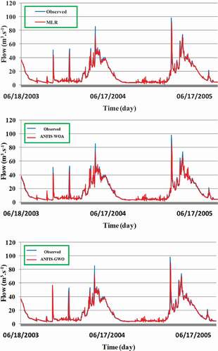
Figure 7. (Continued)

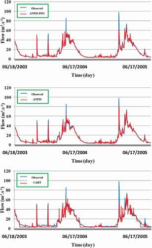
Figure 8. Scatter plot of observed vs. CART, basic ANFIS and meta-optimized hybrid models, ANFIS-GWO, ANFIS-WOA and ANFIS-PSO simulated flow

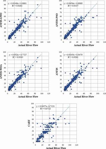
The hybrid model performances were also compared with the performance of two most popularly used algorithms, the MLR and CART models (Fakiola et al. 2010); this comparison revealed better performance of the hybrid models (Table 4). Among the meta-optimized models, the WOA algorithm was found to be the most suitable model. The graphical representations of the observed flow series and those simulated by the proposed models for the validation phase are given in Fig. 7. Visual inspection of the figures indicates that ANFIS-WOA is still very competitive with ANFIS-GWO in reproducing the high flows. All the models were unable to simulate the peak flows. This indicates that the models were not built appropriately to mimic the full scale of the river flow data; in particular they are unable to simulate runoff that occurs due to high-intensity rainfall in the basin. This can be considered a limitation of the proposed models, which researchers can attempt to overcome with the inclusion of more hydrometeorological variables as input in future studies. Although ANFIS-PSO was ranked second after ANFIS-WOA according to evaluation metrics presented in Table 4, it showed a poor performance in reproducing the high flows. Conversely, the ANFIS-GWO was found to reproduce the high flows relatively better despite having higher RMSE.

The WOA algorithm showed superiority over the other metaheuristic algorithms not only because of its capability in avoiding the local optima but also because of its faster convergence. The capability of this algorithm to avoid the local trappings is due to the harmony between the search and exploitation phases, which distinguishes it from other metaheuristic algorithms. The random search for the output variable (Q_t) allowed this trainer to avoid many local optima during learning by the ANFIS model. The hunt encircling mechanism of WOA is another advantage of this algorithm (Aljarah et al. 2018), which provides a more efficient searching strategy compared to other trainers. ANFIS-WOA also showed the fastest convergence compared to ANFIS-GWO and ANFIS-PSO. This is because ANFIS-WOA preserves the best solution and adapts the search around it. Scatter plots of observed and predicted river flow show the highest correlation between the ANFIS-WOA simulation and the observed river flow (Fig. 8). The ANFIS-WOA was able to simulate the observed river flow ranging between 0 and 100 m³.s⁻¹ with a very few deviations. This indicates a good coherence of observed and ANFIS-WOA-predicted river flow. A few deviations might be due to some extreme rainfall events in the basin that caused a sudden change in river flow.

4.6 Statistical analysis

Further discriminative analysis among the models was accomplished using ANOVA, which was conducted to investigate whether there is a meaningful discrepancy between ANFIS-WOA and the other models. The RMSE values of the investigated models were used for the ANOVA test. The test statistics of the models at the 0.05 significance level are provided in Table 5. It was observed that the performance of ANFIS-WOA is significantly different from that of ANFIS-GWO (p value = 0.0002), ANFIS-PSO (p value = 0.006), ANFIS (p value = 0), CART (p value = 0) and MLR (p value = 0). This indicates a meaningful superiority of ANFIS-WOA over the other investigated models. To give a more comprehensible visualization of the performance of the applied predictive models, Fig. 9 presents box plots of the observed daily river flows compared with those simulated using the investigated models. The box height corresponds to the interquartile range and the middle line represents the median of each series. Little variance can be observed based on this graphical presentation. The ANFIS-PSO model reported the minimum outlier observations. The CART model indicated the trend of the data is farther into the first quartile of the box plot. It is clear from the figure that the statistical characteristics of the historical observations are well maintained in the simulations provided by the proposed hybrid models.

Table 5. Results of analysis of variance (ANOVA) test

	ANFIS-GWO	ANFIS-PSO	ANFIS	CART	MLR
p value	.0002	.006	.000	.000	.000

Figure 9. Box plot showing the relative performance of the models

4.7 Validation based on literature review

The results obtained in this study were also validated by comparison with the results of previous studies on river flow forecasting using ML models and their advanced versions. The RMSE metric was used for this purpose. Daily runoff prediction based on ensemble empirical mode decomposition integrated with a heuristic regression model in different regions (i.e. Iran and South Korea; Rezaie-Balf et al. 2019) produced a minimum RMSE of 7.18 and 45.23 m³/s at Kordkheyl and Hongcheon stations, respectively. A hybrid ANN-PSO model was developed for river flow forecasting at Altamaha River, Georgia (Chen et al. 2015), where the model attained a minimum RMSE of 8.15 m³/s. A new hybrid SVM coupled with the fruit fly optimization algorithm (FOA) was developed for runoff prediction at Urmia catchment, Iran (Samadianfard et al. 2019). That study reported minimum RMSEs of 4.36 and 6.33 m³/s at Babarud and Vaniar stations, respectively. The performance of the ANFIS-WOA model in the present study was observed to be better compared to the results presented in previous studies. The RMSE of the ANFIS-WAO model in daily river flow prediction obtained in this study was 3.7 m³/s. This evidences the potential of the proposed ANFIS-WOA model in river flow simulation.

5 Conclusions

River flow pattern is an intricate process controlled by a large number of known and unknown environmental forcing factors. The accuracy of any river flow prediction model is strongly dependent on the efficient optimization of the model parameters. Although ML models are well established for multiscale river flow simulation, improvement of their performance through optimization of their internal parameters is still a new era of intelligent model development. This study proposed the use of metaheuristic optimization algorithms (WOA, GWO and PSO) to develop hybrid ANFIS models for prediction of daily river flow. The hydrometeorological data of the Taleghan River basin situated in the north of Iran was selected to investigate the efficiency of the models. The performance of the proposed models was compared with the standalone ANFIS and CART models. The results demonstrated that meta-optimized hybrid models enhanced the capability of the ANFIS model in the prediction of river flow.

Among the three meta-optimized models, the ANFIS-WOA model was found to be the most suitable model, with the lowest total error in prediction and the fastest convergence speed. The ANFIS-WOA model demonstrated a comparable result with ANFIS-GWO in reproducing the high flows. It improved the predictive capacity of the ANFIS model by 6.5%. The advantage of the ANFIS-WOA model over the other swarm-based and evolutionary-based models is due to its capability of escaping local optima. The model inherits the high exploration capabilities of the WOA algorithm to identify the optimal solution. The results of this study indicate the robustness of the WOA-based trainer in optimizing ML model parameters for better simulation of the daily river flow. However, further studies are encouraged to assess the capability of these models in different regions with diverse complexities.

The results of this study demonstrate that the capabilities of various metaheuristic algorithms differ in simulating the different shapes of hydrographs, and thus, the best model is always not the best in simulating peak flows. This could be a subject of future investigation: to find the best hybrid model which can efficiently reproduce different components of the hydrograph. The performance of only three metaheuristic algorithms is investigated in this study. However, there are many algorithms that can be used in future to achieve a more convincing result in simulating river flow. This study found Q_t-2, Q_t-3 and PG_t-2 to be the least significant input variables and Q_t-1 to be the most important input for river flow simulation. However, determining the best input combination depends heavily on the hydro-environmental characteristics of the study basin. The GT analysis based on the V ratio can be used for determining the best input combination before model construction. Finally, metaheuristic optimization algorithms can be hybridized with other ML models, including ANN and SVM, and their performance can be compared with the hybrid ANFIS model.

Disclosure statement

No potential conflict of interest was reported by the author(s).

References

- Afan, H.A., et al., 2020. Input attributes optimization using the feasibility of genetic nature inspired algorithm: application of river flow forecasting. Scientific Reports, 10 (1), 1–15. Nature Publishing Group. doi:https://doi.org/10.1038/s41598-020-61355-x
- Al-Sudani, Z.A., Salih, S.Q., and Yaseen, Z.M., 2019. Development of multivariate adaptive regression spline integrated with differential evolution model for streamflow simulation. Journal of Hydrology, 573, 1–12. Elsevier. doi:https://doi.org/10.1016/j.jhydrol.2019.03.004
- Aljarah, I., Faris, H., and Mirjalili, S., 2018. Optimizing connection weights in neural networks using the whale optimization algorithm. Soft Computing, 22 (1), 1–15. doi:https://doi.org/10.1007/s00500-016-2442-1
- Anctil, F., et al., 2004. A soil moisture index as an auxiliary ANN input for stream flow forecasting. Journal of Hydrology, 286(1–4), 155–167. Elsevier BV. doi:https://doi.org/10.1016/j.jhydrol.2003.09.006
- Arnold, J.G., et al., 1998. Large area hydrologic modeling and assessment part I: model development. Journal of the American Water Resources Association, 34(1), 73–89. Wiley. doi:https://doi.org/10.1111/j.1752-1688.1998.tb05961.x
- Assareh, E., et al., 2010. Application of PSO (particle swarm optimization) and GA (genetic algorithm) techniques on demand estimation of oil in Iran. Energy, 35(12), 5223–5229. Elsevier BV. doi:https://doi.org/10.1016/j.energy.2010.07.043
- Ayele, G., et al., 2017. Streamflow and sediment yield prediction for watershed prioritization in the Upper Blue Nile River Basin, Ethiopia. Water, 9 (10), 782. doi:https://doi.org/10.3390/w9100782
- Bhagat, S.K., Tung, T.M., and Yaseen, Z.M., 2020. Development of artificial intelligence for modeling wastewater heavy metal removal: state of the art, application assessment and possible future research. Journal of Cleaner Production, 250, 119473.
- Bicknell, B.R., et al., 1997. Hydrological simulation program–Fortran, user’s manual for version 11: U.S. environmental protection agency. Athens, GA: National Exposure Research Laboratory, 755. EPA/600/R-97/080.
- Buragohain, M. and Mahanta, C., 2008. A novel approach for ANFIS modelling based on full factorial design. Applied Soft Computing, 8 (1), 609–625. Elsevier. doi:https://doi.org/10.1016/j.asoc.2007.03.010.
- Chen, W., Panahi, M., and Pourghasemi, H.R., 2017. Performance evaluation of GIS-based new ensemble data mining techniques of adaptive neuro-fuzzy inference system (ANFIS) with genetic algorithm (GA), differential evolution (DE), and particle swarm optimization (PSO) for landslide spatial modelling. Catena, 157, 310–324. doi:https://doi.org/10.1016/j.catena.2017.05.034
- Chen, X.Y., Chau, K.W., and Busari, A.O., 2015b. A comparative study of population-based optimization algorithms for downstream river flow forecasting by a hybrid neural network model. Engineering Applications of Artificial Intelligence, 46, 258–268. doi:https://doi.org/10.1016/j.engappai.2015.09.010
- Chen, X.Y., Chau, K.W., and Wang, W.C., 2015a. A novel hybrid neural network based on continuity equation and fuzzy pattern-recognition for downstream daily river discharge forecasting. Journal of Hydroinformatics, 17 (5), 733–744. doi:https://doi.org/10.2166/hydro.2015.095
- Choubin, B. and Malekian, A., 2017. Combined gamma and M-test-based ANN and ARIMA models for groundwater fluctuation forecasting in semiarid regions. Environmental Earth Sciences, 76 (15). Springer Nature. doi: https://doi.org/10.1007/s12665-017-6870-8
- Croke, B.F.W., et al., 2006. IHACRES Classic Plus: a redesign of the IHACRES rainfall-runoff model. Environmental Modelling & Software, 21(3), 426–427. Elsevier BV. doi:https://doi.org/10.1016/j.envsoft.2005.07.003
- Dehghani, M., Seifi, A., and Riahi-Madvar, H., 2019. Novel forecasting models for immediate-short-term to long-term influent flow prediction by combining ANFIS and grey wolf optimization. Journal of Hydrology, 576, 698–725. Elsevier. doi:https://doi.org/10.1016/j.jhydrol.2019.06.065
- Devia, G.K., Ganasri, B.P., and Dwarakish, G.S., 2015. A review on hydrological models. Aquatic Procedia, 4, 1001–1007. Elsevier BV. doi:https://doi.org/10.1016/j.aqpro.2015.02.126
- Dodangeh, E., et al., 2017. Usability of the BLRP model for hydrological applications in arid and semi-arid regions with limited precipitation data. Modeling Earth Systems and Environment, 3(2), 539–555. Springer Nature. doi:https://doi.org/10.1007/s40808-017-0312-1
- Dodangeh, E., et al., 2019. Data-based bivariate uncertainty assessment of extreme rainfall-runoff using copulas: comparison between annual maximum series (AMS) and peaks over threshold (POT). Environmental Monitoring and Assessment, 191 (2). Springer Nature. doi: https://doi.org/10.1007/s10661-019-7202-0
- Elsafi, S.H., 2014. Artificial neural networks (ANNs) for flood forecasting at Dongola Station in the River Nile, Sudan. Alexandria Engineering Journal, 53(3), 655–662. Elsevier BV. doi:https://doi.org/10.1016/j.aej.2014.06.010
- Evans, D. and Jones, A.J., 2002. A proof of the gamma test. Proceedings of the Royal Society of London. Series A: Mathematical, Physical and Engineering Sciences, 458(2027), 2759–2799. The Royal Society. doi:https://doi.org/10.1098/rspa.2002.1010
- Ewees, A.A. and Elaziz, M.A., 2018. Improved adaptive neuro-fuzzy inference system using gray wolf optimization: a case study in predicting biochar yield. Journal of Intelligent Systems, 29(1), 924–940. Walter de Gruyter GmbH. doi:https://doi.org/10.1515/jisys-2017-0641
- Fakiola, M., et al., 2010. Classification and regression tree and spatial analyses reveal geographic heterogeneity in genome wide linkage study of Indian visceral leishmaniasis. PLoS ONE, 5 (12), e15807. Public Library of Science (PLoS). doi:https://doi.org/10.1371/journal.pone.0015807.
- Farfán, J.F., et al., 2020. A hybrid neural network-based technique to improve the flow forecasting of physical and data-driven models: methodology and case studies in Andean watersheds. Journal of Hydrology: Regional Studies, 27, 100652. Elsevier.
- Faris, H., et al., 2017. Grey wolf optimizer: a review of recent variants and applications. Neural Computing and Applications, 30(2), 413–435. Springer Nature. doi:https://doi.org/10.1007/s00521-017-3272-5
- Firat, M. and Güngör, M., 2007. River flow estimation using adaptive neuro fuzzy inference system. Mathematics and Computers in Simulation, 75 (3–4), 87–96. doi:https://doi.org/10.1016/j.matcom.2006.09.003
- Ghose, D.K., Panda, S.S., and Swain, P.C., 2013. Prediction and optimization of runoff via ANFIS and GA. Alexandria Engineering Journal, 52(2), 209–220. Elsevier BV. doi:https://doi.org/10.1016/j.aej.2013.01.001
- Gupta, H.V., et al., 2009. Decomposition of the mean squared error and NSE performance criteria: implications for improving hydrological modelling. Journal of Hydrology, 377 (1–2), 80–91. doi:https://doi.org/10.1016/j.jhydrol.2009.08.003
- Jaafari, A., et al., 2019. Meta optimization of an adaptive neuro-fuzzy inference system with grey wolf optimizer and biogeography-based optimization algorithms for spatial prediction of landslide susceptibility. CATENA, 175, 430–445. Elsevier BV. doi:https://doi.org/10.1016/j.catena.2018.12.033
- Jacquin, A.P. and Shamseldin, A.Y., 2009. Review of the application of fuzzy inference systems in river flow forecasting. Journal of Hydroinformatics, 11 (3–4), 202–210. doi:https://doi.org/10.2166/hydro.2009.038
- Jang, J.S.R., 1993. ANFIS: adaptive-network-based fuzzy inference system. IEEE Transactions on Systems, Man and Cybernetics, 23 (3), 665–685. doi:https://doi.org/10.1109/21.256541
- Kennedy, J. and Eberhart, R., 1995. Particle swarm optimization. Neural Networks, 1995. Proceedings., IEEE International Conference On, 4, 1942–1948. doi:https://doi.org/10.1109/ICNN.1995.488968
- Khosravi, K., et al. June 2018. Quantifying hourly suspended sediment load using data mining models: case study of a glacierized Andean catchment in Chile. Journal of Hydrology, 567, 165–179. Elsevier. doi:https://doi.org/10.1016/j.jhydrol.2018.10.015
- Končar, N., 1997. Optimisation methodologies for direct inverse neurocontrol. Doctoral dissertation, University of London.
- Kostić, S., et al., 2016. Modeling of river flow rate as a function of rainfall and temperature using response surface methodology based on historical time series. Journal of Hydroinformatics, 18 (4), 651–665. doi:https://doi.org/10.2166/hydro.2016.153
- Leuenberger, M., et al., 2018. Wildfire susceptibility mapping: deterministic vs. stochastic approaches. Environmental Modelling & Software, 101, 194–203. Elsevier BV. doi:https://doi.org/10.1016/j.envsoft.2017.12.019
- Li, X., et al., 2018. Comparison of hybrid models for daily streamflow prediction in a forested basin. Journal of Hydroinformatics, 20 (1), 191–205. doi:https://doi.org/10.2166/hydro.2017.189
- Li, Z., et al., 2016. Impacts of future climate change on river discharge based on hydrological inference: a case study of the Grand River Watershed in Ontario, Canada. Science of the Total Environment, 548–549, 198–210. Elsevier BV. doi:https://doi.org/10.1016/j.scitotenv.2016.01.002
- Maroufpoor, S., et al. February 2019. Soil moisture simulation using hybrid artificial intelligent model: hybridization of adaptive neuro fuzzy inference system with grey wolf optimizer algorithm. Journal of Hydrology, 575, 544–556. Elsevier. doi:https://doi.org/10.1016/j.jhydrol.2019.05.045
- Memarzadeh, R., et al., 2020. A novel equation for longitudinal dispersion coefficient prediction based on the hybrid of SSMD and whale optimization algorithm. Science of the Total Environment, 716, 137007. Elsevier. doi:https://doi.org/10.1016/j.scitotenv.2020.137007
- Meshram, S.G., et al., 2019. River flow prediction using hybrid PSOGSA algorithm based on feed-forward neural network. Soft Computing, 23 (20), 10429–10438. Springer. doi:https://doi.org/10.1007/s00500-018-3598-7.
- Mirjalili, S. and Lewis, A., 2016. The whale optimization algorithm. Advances in Engineering Software, 95, 51–67. doi:https://doi.org/10.1016/j.advengsoft.2016.01.008
- Mirjalili, S., Mirjalili, S.M., and Lewis, A., 2014. Grey Wolf Optimizer. Advances in Engineering Software, 69, 46–61. doi:https://doi.org/10.1016/j.advengsoft.2013.12.007
- Moghaddamnia, A., et al., 2009. Evaporation estimation using artificial neural networks and adaptive neuro-fuzzy inference system techniques. Advances in Water Resources, 32 (1), 88–97. doi:https://doi.org/10.1016/j.advwatres.2008.10.005
- Moriasi, D.N., et al., 2007. Model evaluation guidelines for systematic quantification of accuracy in watershed simulations. Transactions of the ASABE, 50 (3), 885–900. doi:https://doi.org/10.13031/2013.23153
- Muro, C., et al., 2011. Wolf-pack (Canis lupus) hunting strategies emerge from simple rules in computational simulations. Behavioural Processes, 88(3), 192–197. Elsevier BV. doi:https://doi.org/10.1016/j.beproc.2011.09.006
- Napolitano, G., Serinaldi, F., and See, L., 2011. Impact of EMD decomposition and random initialisation of weights in ANN hindcasting of daily stream flow series: an empirical examination. Journal of Hydrology, 406(3–4), 199–214. Elsevier BV. doi:https://doi.org/10.1016/j.jhydrol.2011.06.015
- Nash, J.E. and Sutcliffe, J.V., 1970. River flow forecasting through conceptual models part I - A discussion of principles. Journal of Hydrology, 10 (3), 282–290. doi:https://doi.org/10.1016/0022-1694(70)90255-6
- Pechlivanidis, I.G., et al., 2014. Use of an entropy-based metric in multiobjective calibration to improve model performance. Water Resources Research, 50 (10), 8066–8083. doi:https://doi.org/10.1002/2013WR014537
- Qi, C., et al., 2020. Particulate matter concentration from open-cut coal mines: a hybrid machine learning estimation. Environmental Pollution, 263, 114517. doi:https://doi.org/10.1016/j.envpol.2020.114517
- Rajaee, T., Ebrahimi, H., and Nourani, V., 2019. A review of the artificial intelligence methods in groundwater level modeling. Journal of Hydrology, 572, 336–351. doi:https://doi.org/10.1016/j.jhydrol.2018.12.037
- Rajurkar, M.P., Kothyari, U.C., and Chaube, U.C., 2004. Modeling of the daily rainfall-runoff relationship with artificial neural network. Journal of Hydrology, 285 (1–4), 96–113. doi:https://doi.org/10.1016/j.jhydrol.2003.08.011
- Razavi Termeh, S.V., et al., 2018. Flood susceptibility mapping using novel ensembles of adaptive neuro fuzzy inference system and metaheuristic algorithms. Science of the Total Environment, 615, 438–451. Elsevier BV. doi:https://doi.org/10.1016/j.scitotenv.2017.09.262
- Rezaie-Balf, M., et al., 2019. Daily river flow forecasting using ensemble empirical mode decomposition based heuristic regression models: application on the perennial rivers in Iran and South Korea. Journal of Hydrology, 572, 470–485. Elsevier. doi:https://doi.org/10.1016/j.jhydrol.2019.03.046
- Rezaie-Balf, M., Zahmatkesh, Z., and Kim, S., 2017. Soft computing techniques for rainfall-runoff simulation: local non–parametric paradigm vs. model classification methods. Water Resources Management, 31(12), 3843–3865. Springer Nature. doi:https://doi.org/10.1007/s11269-017-1711-9
- Ritter, A. and Muñoz-Carpena, R., 2013. Performance evaluation of hydrological models: statistical significance for reducing subjectivity in goodness-of-fit assessments. Journal of Hydrology, 480, 33–45. doi:https://doi.org/10.1016/j.jhydrol.2012.12.004
- Roushangar, K., Mehrabani, F.V., and Shiri, J., 2014. Modeling river total bed material load discharge using artificial intelligence approaches (based on conceptual inputs). Journal of Hydrology, 514, 114–122. doi:https://doi.org/10.1016/j.jhydrol.2014.03.065
- Samadianfard, S., et al., 2019. Support vector regression integrated with fruit fly optimization algorithm for river flow forecasting in lake urmia basin. Water (Switzerland), 11 (9). doi:https://doi.org/10.3390/w11091934
- Seifi, A. and Riahi, H., 2020. Estimating daily reference evapotranspiration using hybrid gamma test-least square support vector machine, gamma test-ann, and gamma test-anfis models in an arid area of Iran. Journal of Water and Climate Change, 11 (1), 217–240. doi:https://doi.org/10.2166/wcc.2018.003
- Solomatine, D.P. and Dulal, K.N., 2003. Model trees as an alternative to neural networks in rainfall-runoff modelling. Hydrological Sciences Journal, 48(3), 399–412. Informa UK Limited. doi:https://doi.org/10.1623/hysj.48.3.399.45291
- Solomatine, D.P. and Xue, Y., 2004. M5 model trees and neural networks: application to flood forecasting in the upper reach of the Huai River in China. Journal of Hydrologic Engineering, 9 (6), 491–501. doi:https://doi.org/10.1061/(ASCE)1084-0699(2004)9:6(491)
- Stefánsson, A., Končar, N., and Jones, A.J., 1997. A note on the gamma test. Neural Computing & Applications, 5 (3), 131–133. Springer. doi:https://doi.org/10.1007/BF01413858.
- Tiwari, M.K., et al., 2013. Improving reliability of river flow forecasting using neural networks, wavelets and self-organising maps. Journal of Hydroinformatics, 15 (2), 486–502. doi:https://doi.org/10.2166/hydro.2012.130
- Tiyasha, Tung, T.M., and Yaseen, Z.M., 2020. A survey on river water quality modelling using artificial intelligence models: 2000–2020. Journal of Hydrology. doi:https://doi.org/10.1016/j.jhydrol.2020.124670
- Torabi, S.A., Mastouri, R., and Najarchi, M., 2020. Daily flow forecasting of perennial rivers in an arid watershed: a hybrid ensemble decomposition approach integrated with computational intelligence techniques. Journal of Water Supply: Research and Technology-Aqua, 69 (6), 555–577. doi:https://doi.org/10.2166/aqua.2020.138
- Turan, M.E. and Yurdusev, M.A., 2009. River flow estimation from upstream flow records by artificial intelligence methods. Journal of Hydrology, 369(1–2), 71–77. Elsevier BV. doi:https://doi.org/10.1016/j.jhydrol.2009.02.004
- Watkins, W.A. and Schevill, W.E., 1979. Aerial observation of feeding behavior in four baleen whales: Eubalaena glacialis, Balaenoptera Borealis, Megaptera novaeangliae, and Balaenoptera physalus. Journal of Mammalogy, 60(1), 155–163. Oxford University Press (OUP). doi:https://doi.org/10.2307/1379766
- Yang, Q., et al., 2019. Dynamic runoff simulation in a changing environment: a data stream approach. Environmental Modelling & Software, 112, 157–165. Elsevier BV. doi:https://doi.org/10.1016/j.envsoft.2018.11.007
- Yaseen, Z., et al., 2019. Implementation of univariate paradigm for streamflow simulation using hybrid data-driven model: case study in tropical region: implementation of univariate paradigm for streamflow simulation using hybrid data-driven model: case study in tropical region. IEEE Access, 7, 74471–74481.
- Yaseen, Z.M., et al., 2020. Hourly river flow forecasting: application of emotional neural network versus multiple machine learning paradigms. Water Resources Management, 34 (3), 1075–1091. doi:https://doi.org/10.1007/s11269-020-02484-w
- Zhang, D., et al., 2018. Modeling and simulating of reservoir operation using the artificial neural network, support vector regression, deep learning algorithm. Journal of Hydrology, 565, 720–736. doi:https://doi.org/10.1016/j.jhydrol.2018.08.050